CHANG, HUAN-YU. Damage Visualization of Scattered Ultrasonic Wavefield via Integrated High-speed Camera System (Under the direction of Dr. Fuh-Gwo Yuan).
The ultimate goal for this research is to see through the structure in order to visualize the invisible hidden damages in the structures via camera, so that the damage image can be shown by simply taking a “video” on the structure. Traditionally, for full-field scanning by laser Doppler vibrometer (LDV), the wavefield needs to be reconstructed by measuring each point sequentially. The camera enable measuring all the points at the same time and replacing the current LDV system. However the performance of current high-speed camera is still limited, so for the development of damage imaging algorithm, it needs to be tested with the current laser system.
As the first step in the development of image processing algorithm, a fully non-contact laser scanning system was developed to detect and visualize a barely visible impact damage (BVID) in a honeycomb composite panel. A zero-lag cross correlation (ZLCC) imaging condition was employed for damage imaging. ZLCC results were in very good agreement with ultrasonic C-scan and X-ray CT C-scan results. However, ZLCC was the damage imaging technique based on frequency-wavenumber filtering which requires multiple dimensional Fourier transform, am algorithm for “video” was needed without complex transform and could be operated in time domain.
using the developed imaging condition, named wavenumber index (WI), which is different to other techniques implemented in the frequency-wavenumber domain by the use of complex wavenumber filtering and wave mode decomposition. Since WI is the phase-based imaging technique instead of conventional intensity-based technique for the wavefield “video”, this technique is robust in that the impact damages located in the vicinity of geometry/material discontinuities can yield consistent damage image resolution with high sensitivity even for wave propagating from the direction across the stiffener. The BVID of the composite structure becomes therefore “visible”.
The WI technique was then further applied and integrated with a high-speed camera scanning system, and it successfully visualized the hidden damage through reconstructed scattered wavefield. By employing a sample interleaving and an image stitching technique, the data requisition rate for the high-speed camera was enhanced nearly 250 times in order to overcome the current limited performance due to inadequate on both spatial resolution and temporal resolution, for guided wavefield measurement. Further, many experimental parameters, e.g., specimen design, field of view, speckle size and signal frequency, as well as the camera system were carefully designed, integrated and optimized to enable capture of propagating guided waves excited by a piezo actuator on a surface of the structure. As such the in-plane wave displacements could be maximized and extracted using digital image correlation (DIC).
System
by Huan-Yu Chang
A dissertation submitted to the Graduate Faculty of North Carolina State University
in partial fulfillment of the requirements for the degree of
Doctor of Philosophy
Mechanical Engineering
Raleigh, North Carolina 2019
APPROVED BY:
_______________________________ _______________________________ Dr. Fuh-Gwo Yuan Dr. Chih-Hao Chang
Committee Chair
ii DEDICATION
To my parents who always support me and
iii BIOGRAPHY
Huan-Yu (Tony) Chang is a goal-oriented mechanical engineer and passionate research scientist, who is specialized in automotive engineering, composite structure, finite element analysis (FEA) and nondestructive inspection (NDI).
Tony was born on February 18, 1987, in Taipei, Taiwan. He received his B.S. in 2009 and M.S in 2011, in the Department of Mechanical Engineering at National Taiwan University (NTU). During his college time, he joined the solar car team at NTU, which was later transformed to Formosun Advanced Power Research Center (FAPRC), and started his career path toward an excellent mechanical engineer in automotive industry. He participated the projects building a fuel-cell electric scooter and an electric vehicle (EV), and he was responsible for the entire chassis and part of the structure. In the last year of his grad school, he became the leader of the entire team to finalize the EV project while he was initiating a new project for a new conceptual EV chassis.
After the one-year mandatory military service, Tony started working at Hua-Chuang Automobile Information Technical Center (HAITEC), which is the research and development center of a local automotive company in Taiwan, as a suspension engineer responsible for wheels, tires and the twist beam for the rear suspension.
iv ACKNOWLEDGMENTS
I would like to express my sincere gratitude to my advisor Dr. Fuh-Gwo Yuan for his patient guidance, profound insight, professional attitude and dedication towards researches. Thank you for your support, countless advice and timely response to all my questions. I would also like to thank my committee members: Dr. Chi-Hao Chang, Dr. Larry Silverberg, and Dr. Xiangwu Zhang for your time, advises and helps in completing my dissertation. I also want to thank Dr. Chau-Wai Wong to serve as my substitute committee member in my final defense at a very short notice. Thanks to National Institute of Aerospace for all supports in financial of scholarship, courses, and life helps. I spend meaningful time in National Institute of Aerospace, Virginia.
I would also like to thank the members, graduates and friends in our research group at North Carolina State University: Dr. Jiaze He, Chao Wan, Karthik, and Sakib; Labmate in NIA, Dr. Che-Yuan Chang, Dr. Tyler Hudson, Dr. Yu-Sheng Chang, Dongwon Lee, and Abel Fong. Thank you for all the helpful supports I had with you.
Additionally, I would like to thank all the friends that I have met in Virginia, I could have not continued this long and lonely journey if it wasn’t for all your company.
v TABLE OF CONTENTS
LIST OF TABLES ... v
LIST OF FIGURES ... ix
CHAPTER 1: Introduction ... 1
1.1. Research Motivation ... 1
1.2. Motion Magnification ... 4
1.2.1. Introduction ... 4
1.2.2. Eularian Motion Magnification ... 5
1.2.3. Complex steerable pyramids phase-based motion magnification ... 7
1.2.4. Riesz pyramid phase-based motion magnification ... 10
1.3. Digital Image Correlation ... 12
1.3.1. Digital image correlation in NDI/SHM ... 12
1.3.2. Cross-correlation in displacement extraction ... 16
1.3.3. Comparison of DIC and LDV ... 16
1.4. Guided Waves in Damage Detection for Composites ... 18
1.5. Objectives and Dissertation Outline ... 24
CHAPTER 2: Image Processing via Hilbert and Reisz transform ... 32
2.1. Hilbert Transform ... 32
2.1.1. Introduction ... 32
2.1.2. Definition of Hilbert transform in time domain ... 39
2.1.3. Hilbert transform pairs ... 41
2.1.4. Definition of Hilbert transform in frequency domain ... 43
vi
2.2. Hilbert Spectral Analysis ... 49
2.2.1. Examples for HSA ... 50
2.2.2. Bandlimited signals ... 59
2.2.3. Properties ... 63
2.3. Hilbert-Huang Transform ... 66
2.3.1. Empirical Mode Decomposition and Hilbert Spectrum Analysis ... 66
2.3.2. Limitations and Comparison of HHT ... 80
2.4. Riesz Transform and Monogenic Signal ... 82
2.5. Applications ... 90
2.6. References ... 98
CHAPTER 3: Impact Damage Visualization in a Honeycomb Composite Panel through Laser Inspection using Zero-lag Cross-correlation Imaging Condition ... 104
3.1. Introduction ... 104
3.2. Experimental Study ... 109
3.3. BVID Visualization using Zero-Lag Cross Correlation (ZLCC) Imaging Condition . 120 3.4. Conclusions for ZLCC Imaging Condition ... 134
3.5. References ... 136
CHAPTER 4: Damage Imaging in a Stiffened Curved Composite Sandwich Panel with Wavenumber Index via Riesz Transform ... 140
4.1. Introduction ... 140
4.2. Preliminary Examination ... 146
4.3. Experimental Setup ... 148
vii
4.5. Phase Denoising and Damage Imaging via Wavenumber ... 161
4.6. Results and Comparison ... 163
4.7. Summary and Conclusion ... 166
4.8. Appendix: C-scan Result ... 169
4.9. References ... 170
CHAPTER 5: Damage Visualization of Scattered Ultrasonic Wavefield via Integrated High-speed Camera System ... 174
5.1. Introduction ... 174
5.2. Experiment Setup ... 177
5.3. Logarithmic Value of Wavenumber Index (WI) ... 179
5.4. Results and Comparison- Signal Frequency below the Nyquist Frequency ... 181
5.5. Results and Comparison- Signal Frequency above the Nyquist Frequency ... 185
5.6. Summary and Conclusion ... 189
5.7. References ... 191
CHAPTER 6: Conclusion and Future Work ... 193
6.1. Summary and Conclusion ... 193
viii LIST OF TABLES
Table 1.1. Comparison between LDV and DIC [1.18] ... 18
Table 2.1. Comparison between signal processing methods ... 39
Table 2.2. Selected useful Hilbert transform pairs ... 41
Table 2.3. Properties of Hilbert transform ... 63
Table 2.4. The HHT algorithm ... 74
ix LIST OF FIGURES
Figure 1.1. The procedure to derive the local phase ... 11
Figure 1.2. The illustration of feature tracking at a point ... 15
Figure 1.3. The illustration of feature tracking as a subset ... 15
Figure 2.1. Three-dimensional representation of analytic signal. ... 35
Figure 2.2. (a) The real signal on the time-real plane; (b) the HT on the time-imaginary plane ... 36
Figure 2.3. The analytic signal projected onto the complex plane ... 37
Figure 2.4. The impulse response function h(t) in time domain ... 44
Figure 2.5. The phase response of the impulse response function h(t) ... 45
Figure 2.6 The illustration for envelope and signal ... 49
Figure 2.7. The HT, Envelope and the instantaneous phase ... 50
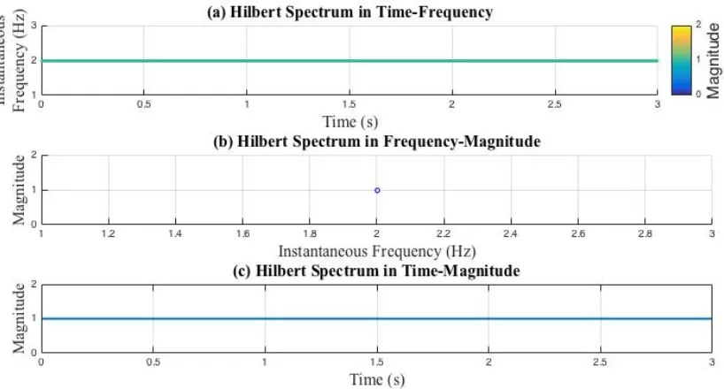
Figure 2.8. The 3-dimensoinal Hilbert spectrum ... 51
Figure 2.9. (a) The time-Frequency, (b) the Frequency-Magnitude, ... 52
Figure 2.10. Chirp signal and its HT and envelope ... 54
Figure 2.11. The instantaneous phase of Chirp signal from HT ... 54
Figure 2.12. The instantaneous frequency of Chirp signal from HT ... 55
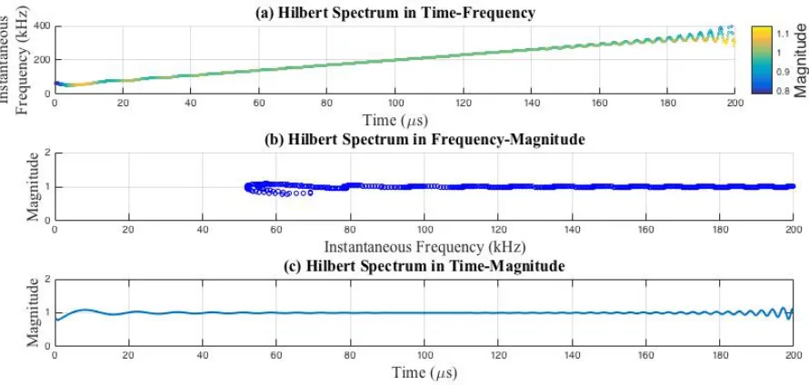
Figure 2.13. The 3-dimensoinal Hilbert spectrum ... 55
Figure 2.14. (a) The time-Frequency, (b) the Frequency-Magnitude, ... 56
Figure 2.15. The Hilbert transform of a 5-cycle Hanning-modulated toneburst signal ... 57
Figure 2.16. The process of HHT ... 67
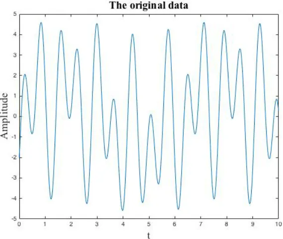
Figure 2.17. The original data ... 68
x
Figure 2.19. The second component h12 of the first IMF ... 70
Figure 2.20. The third component h13 of the first IMF ... 70
Figure 2.21. The first IMF after 6 iterations ... 71
Figure 2.22. The residue of first IMF ... 72
Figure 2.23. The multi-component signal in time domain ... 76
Figure 2.24. The FFT of the multi-component signal ... 77
Figure 2.25. The Hilbert spectrum of the multi-component signal ... 77
Figure 2.26. The numerical (the blue curve) and theoretical (the red curve) IMFs, ... 78
Figure 2.27. The numerical HHT spectrum ... 79
Figure 2.28. The theoretical HHT spectrum ... 79
Figure 2.29. Illustrastion of Riesz transform operator in wavenumber domain along (a) x-axis as shown in Eq.(2.94), (b) y-x-axis as shown in Eq.(2.95). ... 86
Figure 2.30. The illustration of wavefront, orientation and dominant phase direction as described in Eq. (2.99) and (2.100). ... 87
Figure 2.31. The wave filtering and ZLCC imaging method ... 91
Figure 2.32. (a) Frequency-space domain, (b) Instantaneous wavenumber map, (c) Effective thickness map, and (d) Theoretical effective thickness map [2.33].. ... 92
Figure 3.1. Major macro-damage failure modes of a honeycomb composite panel: core/face-sheet disbond, face-sheet delamination and core crush. ... 105
Figure 3.2. A schematic of the NDI system for imaging barely visible impact damage in honeycomb composite panel. ... 110
xi Figure 3.4. The geometry of the composite sandwich panel; (a) perspective view; (b) side
view (units: mm) ... 112
Figure 3.5. Equipment setup for ultrasonic scan of the composite panel: (a) C-scan system, (b) scanning head near the surface of the panel. ... 113
Figure 3.6. Ultrasonic C-scan images of (a) the dent area, (b) the cross-section view and (c) the dent location and size on the composite panel. ... 114
Figure 3.7. (a) Ultrasonic C-scan images of the delamination area, and (b) the delamination location and size on the composite panel. ... 115
Figure 3.8. X-ray CT scan of the impacted honeycomb composite panel: (a) top view from the scanned surface, indicating two elliptical delamination regions 17 mm × 10 mm and 6 mm × 4 mm, and side views from three cross-sections (b) AA, (c) BB, and (d) CC, revealing the depth and shape of the delaminations. ... 117
Figure 3.9. Excitation signal in the honeycomb composite panel generated by the pulse laser was measured by a nearby LDV. ... 119
Figure 3.10. Wavefield in the honeycomb composite panel at t = 265 𝜇s: (a) prior to impact; (b) after impact. ... 120
Figure 3.11. Wavenumber map at each frequency ... 123
Figure 3.12. Quadrant filtered wavenumber map ... 124
Figure 3.13. Filtered reflected wavefield at t = 265 s. ... 126
Figure 3.14. Damage image using a simple RMS of out-of-plane velocity response ... 127
xii Figure 3.16. The damage imaged using ZLCC imaging condition at (a) 25 kHz, (b) 55 kHz,
(c) 80 kHz. ... 129 Figure 3.17. The wavenumber map showing standing wave phenomenon at (a) 25 kHz, (b)
55 kHz, (c) 80 kHz. ... 130 Figure 3.18. Local resonant result from FEA (a) First mode around 24 kHz; (b) Second
mode around 55 kHz. ... 132 Figure 3.19. The damage image using ZLCC imaging condition summed over the
frequency range, 0-50 kHz. ... 133 Figure 3.20. The damage image using ZLCC imaging condition summed over the
frequency range, 80-95 kHz. ... 133 Figure 4.1.(a) The geometry of the stiffened curved composite foam panel (not-to-scale),
(b) The illustration of ball-drop impact test, (c) The illustration for the cross
section of the impact damage region close to the stiffener (not-to-scale). ... 147 Figure 4.2. The ultrasonic C-scan experimental setup and the result for the impact damage.
... 148 Figure 4.3. A schematic of laser scanning system for imaging the barely visible impact
damage ... 149 Figure 4.4. The illustration of LDV locations, scanning area and the crosssection of the
panel ... 150 Figure 4.5. Excitation signal in the honeycomb composite panel generated by the pulse
laser was measured by a nearby LDV. ... 151 Figure 4.6. The wavenumber map of the wavefield excited from four locations shown in
xiii damage region. (a) #1, rightward, (b) #2, leftward, (c) #3, downward and (d)
#4, upward. ... 152 Figure 4.7. The snapshot of the wavefield “video” for (a) #1, rightward, (b) #2, leftward,
(c) #3, downward and (d) #4, upward. ... 154 Figure 4.8. Illustrastion of Riesz transform operator in wavenumber domain along (a)
x-axis as shown in Eq. (4.5), (b) y-x-axis as shown in Eq. (4.6). ... 157 Figure 4.9. The illustration of wavefront, orientation and dominant phase direction as
described in Eq. (4.10) and (4.11). ... 159 Figure 4.10. ZLCC results for LDV location and wave propagting direction: (a) #1,
rightward, (b) #2, leftward, (c) #3, downward and (d) #4, upward. ... 164 Figure 4.11. WI results for LDV location and wave propagting direction: (a) #1, rightward,
(b) #2, leftward, (c) #3, downward and (d) #4, upward. ... 165 Figure 4.12. The C-scan result shows all the delaminations at different depths beneath the
impact location. ... 169 Figure 5.1. (a) The schematic system layout of experimental setup, and (b) the illustration
of specimen setup in the test ... 178 Figure 5.2. Frequency spectrum for 14kHz excitation at an arbitrary point before filtering
for (a) displacement, and (b) y-displacement; after filtering for (c)
x-displacement, and (d) y-displacement ... 182 Figure 5.3. The wavefield snapshot at 800 μs for (a) ux, (b) uy from camera, and (c) uz from
LDV. The red dotted rectangle indicates the simulated damage at the back of
xiv Figure 5.4. The damage image generated from wavefield in (a) SH mode from camera, (b)
S0 mode from camera, and (c) A0 mode from LDV. The red dotted rectangle
indicates the simulated damage at the back of the plate. ... 184 Figure 5.5. Frequency spectrum for 28kHz excitation at an arbitrary point before filtering
for (a) displacement, and (b) y-displacement; after filtering for (c)
x-displacement, and (d) y-displacement ... 186 Figure 5.6. The damage image generated from reconstructed wavefield via camera in (a)
SH mode, (b) S0 mode. The red dotted line indicates the simulated damage at
the back of the plate. ... 187 Figure 5.7. The damage image generated from reconstructed wavefield via camera in (a)
SH mode, (b) S0 mode. The red dotted line indicates the simulated damage at
1 CHAPTER 1 Introduction
1.1. Research Motivation
Visual inspection is the most traditional and intuitive non-destructive inspection (NDI) method with long history and remains the most economical as well as fastest way for early assessment of health conditions of aircrafts [1.1]. Currently, over 80 percent of the inspections on large aircraft are done visually. As the time goes, visual inspection has evolved and been improved with the assistant of advanced technologies. Camera has been introduced to record the inspecting process, capture the image of the object and keep track of the history, providing better reliability, confidence, and somewhat automation. Recently, with the developed computer vision technique, camera has replaced human being in the inspection during manufacture or production. However, for the aviation industry, the visual inspection still relies on the knowledge and experience of the inspection personnel, and requires subjective judgement, both of which tend to be labor-intensive, tedious and inconsistent.
2 visualized. The nearly invisible impact damage has increased the difficulty of visual inspection of composite structures for aircrafts and result in more time consumption, higher cost and even riskier.
Although some NDI techniques such as ultrasound C-scan and X-ray CT have shown to be effective in detecting such minute damages, they suffer disadvantages of being extremely costly and time-consuming. In most cases, the equipment is non-portable and the disassembly of the parts is required due to the limitation of dimension, which makes these techniques not suitable for early estimation of structural condition. Piezoelectric transducers and optical fibers are compact and lightweight with good sensitivity that can be used to detect anomalies in the structure by attaching/embedding them on/in the structure; however, the deployment of sensors and the wiring can be an issue as the amount of sensors increases. The fully non-contact, efficient and flexible techniques are hence highly preferred for the inspection of composite structures.
3 For now LDV can be considered the most reliable and comprehensively used remote sensing technique providing precise measurement, but the technique also reveals several additional pitfalls in inhibiting practical area scanning: (1) the point-by-point scanning over the damage region by the LDV system is time-consuming; (2) the signal or event recorded by LDV must be absolutely repeatable or stationary; and (3) repeated excitations for the sampling may deteriorate the structure further after the inspection. At present, none of these NDI techniques can provide non-contact remote robust sensing capability to the inspection for composite structures of aircrafts.
4 several successful applications of digital cameras in NDI have been shown recently, none of them can meet the requirement of both spatial and temporal resolution for the inspection in composite structures due to the limitation of current technology.
In this dissertation, the ultimate goal is to overcome the limitation of the current hardware by increasing the equivalent sampling frequency and resolution of the high-speed camera, so that the concept of using camera for damage detection and visualization can be proved. Even though there are several damage imaging condition that have been developed to visualize the hidden damage using guided wavefield, these imaging conditions possess certain disadvantages. Therefore a new technique is needed for improving the sensitivity and flexibility, and it can be further customized for the wavefield captured by the high-speed camera. Once the new camera is developed in the near future, the algorithm and technique developed in this dissertation can be accommodated to the latest technique to achieve the goal of real-time damage visualization using high-speed camera.
1
1.2. Motion Magnification
1.2.1. Introduction
5 There are several different techniques can achieve the goal. Eulerian motion magnification method was developed mathematically based on first-order linear Taylor-series expansion in 2012 [1.2], which was fast and simple, but limited in scaling factor and sensitive to noise characteristic. To avoid the noise from being magnified, complex steerable pyramids phase-based motion magnification was then developed [1.3] for increasing scaling factor and signal-to-noise (SNR) behavior, but it was computationally costly due to the over-completeness caused by multi-orientation. Therefore, Riesz-pyramid was brought up [1.4] to replace the complex steerable pyramids for the computational efficiency while keeping similar image quality.
The motion magnification method has been recently applied to some research relevant to structural health monitoring. However, it was mostly just used for simple beam-like one-dimensional problem, and the application for composite plate still has not been discussed yet.
1.2.2. Eularian Motion Magnification
6 After being decomposed, I(x,0) is the initial intensity of the pixel located at coordinate x, and I(x,t) is the intensity at the instant t. Assuming that the image undergoes a translational motion, the intensity of the pixel was moved for δ(t). The intensity initially located at x, after a period of time t, moves to the new location of x+δ(t). Then the intensity can be expressed with respect to the displacement function δ(t).
(1.1)
By applying the first-order Taylor series expansion, the intensity at time t can be expressed as
(1.2)
In order to pick out the displacement signal, a spatial bandpass filter was applied to the intensity function and the signal was extracted as
(1.3)
Giving a magnifying factor α, the bandpass signal B(x,t) can be multiplied by α and added back to
I(x,t), the processed signal can be written as
(1.4)
The processed signal can be applied with first-order Taylor expansion again, the signal then can be expressed as
I(x,0)= f(x) ⇒ I(x,t)= f(x+δ(t))
I(x,t)≈ f(x)+δ(t)∂f(x) ∂x
B(x,t)=δ(t)∂f(x) ∂x
!
I(x,t)
!
I(x,t)≈ f(x)+(1+α)δ(t)∂f(x) ∂x
!
7 This shows that the processing magnifies motions the spatial displacement δ(t) of the local image f(x) at time t, has been magnified to a magnitude of (1+α). After being processed, the intensity value initially at coordinate x moves to x+δ(t) originally, but now moves to x+(1+α)δ(t) instead.
(1.5)
The limitation of Eulerian motion magnification arises from the linear approximation of the first-order Taylor series expansion. Due to the linear approximation, the error cannot be neglected when the displacement becomes large. Even though the Eulerian motion magnification is a simple method with fast processing, it is limited to small magnification factor, especially for high spatial frequency case and it is highly sensitive to noises. The disadvantages of linear approximation limit the feasibility of this method. Therefore the phase-based technique was further developed to circumvent the problem and to increase the feasibility and image quality.
1.2.3. Complex steerable pyramids phase-based motion magnification
As mentioned previously, Eulerian motion magnification method is based on linear approximation of first-order Taylor series expansion, which leads to the sensitivity to noises and the limited magnification factor. The phase-based motion magnification technique was then developed for overcoming the disadvantages, which was based on Fourier series decomposition.
Similar to the Eulerian motion magnification, the goal of phase-based motion magnification method is to extract the displacement function from the intensity function and to create the displacement-magnified intensity function.
8 (1.6)
As described in the previous part, the intensity function initially located at x is defined as I(x,0), and the intensity at the instant time t is also defined as I(x,t). By applying Fourier serious decomposition, the two intensity function can be decomposed to a summation of a series of complex exponential functions.
(1.7)
(1.8)
After Fourier series decomposition, each sub-band Sk(x,t) corresponds to a single spatial frequency k, and the phase term k[x+δ(t)] contains the motion information.
(1.9)
By applying a temporal filter, the DC component kx will be removed, and the residue is the bandpassed phase Bk(x,t). The bandpassed phase can then be multiplied by the amplifying factor α for increasing the phase of sub-band Sk(x,t).
(1.10)
The spatial displacement δ(t) of the local image f(x) at time t has been magnified by (1+α). The reason why phase-based motion magnification method has less sensitivity to noises is that the motion is magnified by shifting the phase, and the magnitude will not change during the process. Assuming the sub-band signal with noise is
I(x,t)= f(x+δ(t)) ⇒ I!(x,t)≈ f(x+(1+α)δ(t))
I(x,0)= f(x) FFT⇒ Aωeiωx ω=−∞
∞
∑
I(x,t)= f(x+δ(t)) ⇒FFT Akeiω(x+δ( )t) ω=−∞
∞
∑
Sk(x,t)= Akeik(x+δ(t))
ˆ
Sk(x,t)=Sk(x,t)eiαBk = A ke
ik(x+δ(t))eiαkδ(t) = A
ke
9 (1.11)
As the previously mentioned procedure, the motion can be magnified by following procedure.
(1.12)
The noise in the signal is only phase-shifted instead of being magnified. Therefore the phase-based technique can effectively solve the noise problem of linear approximation method.
To get the local phase and local translation, a quadrature pair is derived to form a complex number for using the Fourier phase shift theory; therefore, Hilbert transform can be used as a phase shifter.
(1.13)
For any frequency k, the Hilbert transform of fx=coskx is gx=sinkx, implying Hilbert transform is a phase shifter, which gives any sinusoidal function -90° of phase shift. Considering all the motion as a cosine function, then we can get its quadrature pair, which is a sine function, after the Hilbert transform.
(1.14)
After the same phase shifting, the function will go forward for positive spatial frequency and go backward for negative spatial frequency.
(1.15) Sk(x,t)= Akeik(x+δ(t))+σ
nNk(x,t)
ˆ
Sk(x,t)=Sk(x,t)eiαBk = A
ke
ik(x+(1+α)δ(t))+σ
ne iαkδ(t)N
k(x,t)
H{cos(kx)}=cos(kx−π
2)=sin(kx) ⇒ cos(kx)+isin(kx)=e ikx
for k>0 ⇒ eikxe−iφ =ei(kx−φ), which is shifted forward
10 This phase-based motion magnification method introduced the concept to connect the magnitude and direction of the motion with the spatial phase derived from the image, and the maginified images obtained with the technique showed promising results to prove the feasibility and practicability. However, the phase is only defined in one dimension. There are at least two orientations needed to obtain the phase and orientation information from images, and in order to increase the accuracy of the reconstructed magnified images, typically more than eight orientations are used to ensure the precision, which leads to more computational cost. Therefore the Riesz transform was further introduced to the phase-based method to reduce the computational time while keeping the image quality.
1.2.4. Riesz pyramid phase-based motion magnification
Even though the complex steerable pyramid phase-based method resolved the problems of the sensitivity to noises and the limitation of magnifying factor for the Eulerian motion magnification based on liner approximation, it is much more computational costly for the multiple orientation of the steerable complex pyramid. The Riesz pyramid method is still a phase-based technique, but the Riesz pyramid is used for decomposition instead of original complex steerable pyramid.
11 (1.16)
By applying Riesz transform, the 90° phase-shift in two orientations can be generated from the input sub-band. The dominant orientation can be further computed for each location from the two transforms. After getting the quadrature mate, the quadrature pair is formed and the local phase is known. Therefore the method can be computationally efficient without processing in frequency domain.
Figure 1.1. The procedure to derive the local phase
Assume the input sub-band function is I=Acosϕ , where A is amplitude and ϕ is local phase. The two Riesz transform results are R1=Asinϕcosθ and R1=Asinϕsinθ , where θ is dominant orientation. The direction is invariant because of steerability, when arbitrary rotation angle θ0 equals to local dominant orientation θ, the first component becomes the quadrature mate Q=Asinϕ. The local dominant orientation and local phase for each point can thus be found for generating quadrature pair and applying phase-based motion magnification technique.
−i kx k
12
(1.17)
The Riesz pyramids method is still based on phase-based motion magnification, while using the Riesz pyramids in the spatial domain to replace the Complex Steerable Pyramids. After magnification, the noise characteristic and the magnification factor can almost keep the same as phase-based method while being much more computationally effective. This phase-based method with Riesz pyramid showed the effectiveness of deriving spatial phase and frequency, which gives a promising preliminary result for further analysis on wavefields using Riesz transform.
1.3. Digital Image Correlation
1.3.1. Digital image correlation in NDI/SHM
For damage detection, visualization and identification, traditionally signals are excited/measured on the surface for structural dynamic measurement by either contact or non-contact methods, e.g., a discrete piezo sensor array, the Nd-YAG pulse laser, and the laser Doppler vibrometer (LDV), and the signals are required to be linear, stationary and repeatable in order to reconstruct full-field signals from the point-by-point measurement, especially for guided wavefield reconstruction [1.6]. Guided wave-based techniques have been comprehensively employed to non-destructive inspection (NDI), structural health monitoring (SHM), and material characterization in plate-like structures [1.7]. However, current systems that can measure full wavefield propagation require significant set-up time, and collecting signal or scanning wavefield is time-consuming.
cos
( )
θ0 sin( )
θ0 −sin( )
θ0 cos( )
θ0 ⎡ ⎣ ⎢ ⎢ ⎤ ⎦ ⎥ ⎥ R1 R2 ⎡ ⎣ ⎢ ⎢ ⎤ ⎦ ⎥ ⎥=Asinφcos
(
θ−θ0)
13 Digital image correlation (DIC) is the solution that can circumvent these problems. The DIC technique is an optical technique employing feature tracking and image registration for extracting full-field displacement and strain fields from the change in images. The technique has been comprehensively applied for research and industrial testing purpose, and the recent advances in the camera technology and computer performance have been broadening the applicable field that requires high spatial and temporal resolution [1.8]. As the technology improves, the new high-speed cameras nowadays are showing good potentials to achieve full-field measurement for transient signals and to provide the most spatially continuous sampling compared to any other measurement methods with discrete sensing locations.
14 1.3.2. Cross-correlation in displacement extraction
Using cross-correlation for obtaining differences and correlations between datasets has been known for a long time, and the earliest application in dealing with digital images is known as in 1970s [1.10]. Some research and development of DIC in early phase was conducted by a group of researchers at the University of South Carolina (USC) in 1980s [1.11], and its DIC algorithm has been optimized and improved recently and has become a mature product in the industry and academy.
15 Figure 1.2. The illustration of feature tracking at a point
Figure 1.3. The illustration of feature tracking as a subset
For the full-field displacement extraction, the main task is to find where each subset moved by checking possible matches at several locations with a correlation function to obtain the maximum similarity between the deformed and undeformed images. The most classic correlation function is the sum of squared differences (SSD) of the pixel values, where the smaller value stands for better similarity between two subset. The basic SSD function C(x,y,u,v) is shown in Eq.(1.18), where (x,y) is the pixel coordinate in the undeformed image, (u,v) is the displacement of the subset in the
Time t1 Time t2 Time t3
Feature tracking
Feature tracking Feature tracking
Time t1 Time t2 Time t3
Feature tracking
16 deformed image, n is the subset size, and I and I* are the pixel value for the undeformed and deformed images. For perfect matching, the SSD value will be zero, which is the smallest value achievable. However, in real application, the value will never be zero because the images are always corrupted by noise. Interpolation technique will be needed in real application for images at non-integer pixel location.
(1.18)
1.3.3. Comparison of DIC and LDV
Laser Doppler vibrometer (LDV) is one of the mature methods for collecting experimental measurements at discrete locations, and it has become well established in the vibrational, modal and wave analysis. Other optical measurement technique like digital image correlation (DIC) is relatively new in these applications. The main difference between LDV and DIC is that the LDV is only able to measure one point at each time, but DIC can measure multiple points within the measurement region simultaneously. Therefore, the measurement via LDV requires the excitation signal to be linear, stationary and repeatable in order to simulate that the reconstructed signal is measured at multiple points at the same time. The sequential measurement at each points for LDV requires longer times for obtaining the data, but the data itself is formatted and ready for further post-processing. In contrast, the DIC is time-efficient in measuring the data and it is able to deal with transient signal since it captures all the points at the same time, but the images obtained from camera require further correlation calculation in order to extract the full-field displacement. Therefore the computational time for DIC is humongous.
C(x,y,u,v)= (I(x+i,y+ j)−I*(x+u+i,y+v+ j))2 i,j=−n/2
17 Recent studies [1.14][1.15] have shown the possibility of using DIC in vibrational analysis, and DIC is found to be capable of generating full-field data from measurement. Other studies [1.16][1.17] have done comparison between LDV, DIC and traditional accelerometers for generating data in the experiment of modal analysis. Reu et al. [1.18] has recently done a detailed comparison of DIC and LDV with discussion for the pros and cons of each technique in practical vibration and modal measurement.
18 Table 1.1. Comparison between LDV and DIC [1.18]
Comparison Metric LDV DIC
Cost ~$650k ~$350k
Setup Time 2 hours 2 hours
Acquisition Time Hours Seconds
Analysis Time Seconds Hours
Disp. Resolution ~Picometers ~Nanometers
Strain Resolution N/A 5 micron
Strain Calculation Integrated- but researchy Seamlessly integrated Anti-aliasing Included Not possible at the moment
Data Volume Small (Mbytes) includes only frequency data
Large (Gbytes) but includes time history
Software Designed for
structural dynamic testing
In its infancy
1.4. Guided Waves in Damage Detection for Composites
19 Unavoidable impacts occur to aircrafts during in-service operation, such as bird strikes or hail impacts. Furthermore, accidents may happen to regular inspection or maintenance leading to unexpected damages. For aluminum or steel structures, these impacts may cause dents or deformation on the surfaces with negligible reduction in strength or stiffness; however, for composite structures, impact load may cause delamination and debonding beneath surfaces, or even crush for the core material that can deteriorate the mechanical performance of materials significantly. These impact damages in composite materials are barely visible from the appearance, and they are difficult to be found during regular visual inspection, leading to potential safety issues and higher risk. Even though there are several robust non-destructive inspection (NDI) techniques that can not only detect but also visualize aforementioned barely-visible impact damage (BVID) in composites, such as ultrasonic scan or X-ray computed tomography (CT) scan, they are mostly not portable and time-consuming, and the techniques have spatial limitation that requires disassembly of the interrogated objectives [1.19].
20 damages by comparing the wave signals between pristine condition and damaged condition. Once the amount of sensor/actuator increases, the damages can be further located; array configuration is commonly used recently for damage localization than distributed sensor/actuator [1.20]. When the amount of the sampling point is large enough with ideal sampling spacing, the wave signal measured at each point can be reconstructed as a wavefield. The detailed shape and location of the damage can be visualized by analyzing the wavefield with a damage imaging technique.
Several damage imaging methods have been developed lately for damage visualization based on guided wavefield. Ruzzene et al. [1.21] first introduced root-mean-square (RMS) method which is the square root of the average sum of the wave signals squared, as shown in Eq.(1.19), to highlight the intensity difference at the damaged region for damage imaging. RMS can be considered as the most intuitive and simple method for damage imaging, it was further improved by Zak et al. [1.22] with weighted RMS and Saravanan et al. [1.23] with radially weighted and factored RMS for better damage imaging results.
(1.19)
where wT(x,y,t) is the total wave signal, ti is the initial time of the interested period, and N is the amount of sampling point of the interested period. Sohn et al. [1.24] , An et al. [1.25] and Park et al. [1.26] proposed a cumulative total wave energy (CTWE) technique with similar concept of RMS and a cumulative standing wave energy (CSWE) that shows more physical meaning to highlight local resonance behavior for damage visualization in composites. The standing wave energy is defined as the total wave signal squared minus the sum of propagating wave signals squared in four quadrants that were separated in frequency-wavenumber domain, as expressed in
RMS(x,y)= 1
N wT
2(x,y,t i) i=1
21 Eq.(1.20). Then the cumulative standing wave energy is the integration of the standing wave energy within the interested sampling period as shown in Eq.(1.21).
(1.20)
where wT(x,y,t) is the total wave signal, and wp(x,y,t) is the propagating wave signal for p=1,2,3,4.
(1.21)
where T is the sampling period of interest.
Instead of using the localized high value in the amplitude of wavefield to highlight the damage region, Yuan and Harb [1.27][1.28] first introduced a zero-lag cross-correlation (ZLCC) damage imaging technique, where the incident and reflected waves separated in the frequency-wavenumber domain were cross-correlated with zero time-lag to generate a cumulative damage image, as shown in Eq.(1.22). The incident wave and reflected waves are separated with a wavenumber filter along the interested direction, and ZLCC show the highest correlation value at the boundary of the damage where the reflected waves are generated. Girolamo et al. [1.29] further redefined the forward and backward propagating waves in improved two-dimensional wavenumber filtering process and employed ZLCC in frequency domain, as Eq.(1.23), to highlight the local resonant vibration within the damage region on a honeycomb composite panel. ZLCC employed in frequency domain shows better damage imaging result with less ambient noise and is capable of extracting the hidden resonant behaviors at higher local resonant frequencies.
SWE(x,y,t)=wT2(x,y,t)− w p
2(x,y,t) p=1
4
∑
CSWE(x,y)=
0 T
22 (1.22)
where winc and wref are incident and reflected, respectively, wave signal in time-space domain separated with frequency-wavenumber filter.
(1.23)
where winc and wref are incident and reflected, respectively, wave signal in frequency-space domain
separated with frequency-wavenumber filter, and wi, wf are lower and upper frequency respectively of the interested frequency range.
Furthermore, there are several damage imaging conditions taking advantage of localized wavenumber value to highlight the discontinuity in mechanical properties. Rogge and Lecky [1.30] introduced a wavenumber domain analysis via a mode separation technique followed by a spatial-windowed Fourier transform to obtain local wavenumber from the wavefield for characterization of impact damages in a composite plate. The developed wavenumber domain analysis provide good agreement with theoretical prediction of spatial window selection, and the damage imaging result shows the capability to characterize the depth of the delamination in composite laminate. Then the technique was further enhanced by Juarez and Lecky [1.31] to multi-frequency local wavenumber analysis along with a ply correlation technique to quantify the impact damage. With similar concept of using localized wavenumber to highlight the damage region, Mesnil et al. [1.32] proposed an instantaneous wavenumber estimation method for damage quantification, by employing one-dimensional spatial Hilbert transform on the wavefield for obtaining instantaneous wavenumber, as shown in Eq.(1.24), where k(x,t) is the instantaneous wavenumber, is the
I(x,y)= winc
0
T
∫
(x,y,τ)wref(x,y,T −τ)dτI(x,y)= winc ω=ωi
ωf
∑
(x,y,ω)wref*(x,y,ω)
23 Hilbert transformed signal of wave signal w(x,y). The two-dimensional instantaneous wavenumber generalization was then defined as the square root of the sum of instantaneous wavenumber squared in two directions as shown in Eq.(1.25).
(1.24)
(1.25)
Flynn et al. [1.33] introduced a damage imaging condition using local wavenumber estimation to image the structural features and defects. A wave mode separation technique was first applied onto the wavefield signal to isolate a narrow-band and single mode wave signal with its central
frequency fc and central wavenumber kc, and local wavenumber were defined as the
highest magnitude of the space-wavenumber representation for each point, as shown in Eq.(1.26). The space-wavenumber representation S(x,y,kc) at given central wavenumber kc is calculated by the sum of three-dimensional monogenic envelops of filtered wavefield signal at central wavenumber kc within the interested sampling period as Eq.(1.27).
(1.26)
(1.27)
where w(x,y,t,kc) is the wavefield signal with central wavenumber kc, is the 3-D monogenic
envelope, t0 is initial sampling time, and T is the total sampling period. k(x,t)=imag
∂wˆ(x,t) ∂x
ˆ w(x,t)
⎛ ⎝⎜
⎞ ⎠⎟
IW(x,y,t)= kx2(x,y,t)+k y
2(x,y,t)
ˆ
kLOC(x,y)
ˆ
kLOC(x,y)=arg max k
S(x,y,k)
S(x,y,kc)= w(x,y,t,kc) E t=t0
T
∑
24 In this dissertation, a new guided wave-based damage visualization method employing Riesz transform as an image processing technique was developed by the author and applied on a stiffened curved composite panel. The developed damage imaging technique, named wavenumber index (WI), took advantage of the abundant information contained in monogenic signals representation of the guided wavefield. The monogenic signal was derived by Riesz transform, the genuine two-dimensional generalized Hilbert transform in space domain, to obtain instantaneous orientation, phase and amplitude of the constructed guided wavefield. The instantaneous wave energy was calculated from instantaneous amplitude, and the instantaneous wave vector was obtained by taking derivative with respect to two axes in space domain. The detailed description of WI method will be provide in Chapter 4.
1.5. Objectives and Dissertation Outline
The ultimate goal of this dissertation is to develop a robust fully noncontact vision-based NDI technique as a solution to remotely monitor the integrity and diagnose hidden damages in composite structures for aircrafts. The developed vision-based NDI system consists of (1) high-speed digital cameras with optimized illumination and surface treatment technique for the best sampling quality, (2) an automated scanning system for the rapid and effective diagnosis of large structures, and (3) the processing/controlling system to identify and visualize invisible damages via newly developed image processing technique.
25 condition are also provided in this chapter. The Hilbert transform and Riesz transform, which are two important keys in the technique of motion magnification, are introduced in details in chapter 2. Hilbert transform is a powerful time-frequency analysis tool that can be comparable with other methods such as short-time Fourier transform and Wavelet transform. The theory will be described and examples will also be given in the following chapter. The extension of Hilbert transform: Hilbert-Huang transform and Riesz transfom are both able to be applied for imaging processing will also be introduced in the next chapter.
26 scanned region. The condition not only imaged the damage boundary between incident and reflected waves outside the damage region but also, for longer time windows, enabled to capture the momentary standing waves formed within the damaged region. The ZLCC imaging condition imaged two delaminated region: a main delamination, which was a skewed elliptic with major and minor axis lengths roughly 17 mm and 10 mm respectively, and a secondary delamination region approximately 6 mm by 4 mm, however, which could only be shown at higher frequency range around 80 kHz to 95 kHz. To conclude, the ZLCC results were in very good agreement with ultrasonic C-scan and X-ray computed tomographic (X-ray CT) scan results. Since the imaging condition was performed in the space-frequency domain, the imaging from ZLCC could also reveal resonance modes which were shown in the main delaminated area by windowing a narrow frequency band sequentially.
28 1.6. References
[1.1] Visual inspection for aircraft, Advisory Circular 43-204, Federal Aircraft Administration, 1997.
[1.2] H. Y. Wu, M. Rubinstein, E. Shih, J. Guttag, F. Durand, and W. Freedom, ”Eulerian Video Magnification for Revealing Subtle Changes in the World,” 2012.
[1.3] N. Wadhwa, M. Rubinstein, F. Durand, and W. T. Freeman, “Phase-based Video Motion Processing,” ACM Transactions on Graphics, vol.32, no.4, pp.80:1–80:10, 2013.
[1.4] N. Wadhwa, M. Rubinstein, F. Durand, and W. T. Freeman, ”Riesz Pyramid for Fast Phase-based Video Magnification,” Computational Photography (ICCP), 2014 IEEE International Conference on. IEEE, pp. xx-xx, 2014.
[1.5] K. Kamble, N. Jagtap, R.A Patil and A. Bhurane, “A Review: Eulerian Video Motion Magnification,” International Journal of Innovative Research in Computer and Communication Engineering, vol.3, no.3, 2015.
[1.6] D. Girolamo, H.Y Chang, and F.G. Yuan, “Impact Damage Visualization in a Honeycomb Composite Panel through Laser Inspection using Zero-lag Cross-correlation Imaging Condition,” Ultrasonics, vol.81, pp.152-165, 2018.
[1.7] H.Y. Chang and F.G. Yuan, “Impact damage imaging in a curved composite panel with wavenumber index via Riesz transform,” Proc. SPIE 10599, Nondestructive Characterization and Monitoring of Advanced Materials, Aerospace, Civil Infrastructure, and Transportation XII, p.105990L, 2018.
29 [1.9] F. Trebuňa and M. Hagara, “Experimental modal analysis performed by high-speed digital
image correlation system,” Measurement, vol.50, pp.78-85, 2014.
[1.10]P.E. Anuta, “Spatial registration of multispectral and multitemporal digital imagery using fast Fourier transform techniques,” IEEE transactions on Geoscience Electronics, vol.8,
no.4, pp.353-368, 1970.
[1.11]M.A. Sutton, C. Mingqi, W.H. Peters, Y.J. Chao and S.R. McNeill, ”Application of an optimized digital correlation method to planar deformation analysis,” Image and Vision
Computing, vol.4, no.3, pp.143-150, 1986.
[1.12]H.W. Schreier and M.A. Sutton, “Systematic errors in digital image correlation due to undermatched subset shape functions,” Experimental Mechanics, vol.42, no.3, pp.303-310,
2002.
[1.13]B. Pan, H. Xie, Z. Wang, K. Qian and Z. Wang, “Study on subset size selection in digital image correlation for speckle patterns,” Optics express, vol.16, no.10, pp.7037-7048, 2008.
[1.14]M.N. Helfrick, C. Niezrecki, P. Avitabile, P. and T. Schmidt, “3D digital image correlation methods for full-field vibration measurement,” Mechanical systems and signal
processing, vol.25, no.3, pp.917-927, 2011.
[1.15]W. Wang, J.E. Mottershead, T. Siebert and A, Pipino, “Frequency response functions of shape features from full-field vibration measurements using digital image
correlation,” Mechanical systems and signal processing, vol.28, pp.333-347, 2012.
[1.16]C. Warren, C. Niezrecki, P. Avitabile and P. Pingle, ”Comparison of FRF measurements and mode shapes determined using optically image based, laser, and accelerometer
measurements,” Mechanical Systems and Signal Processing, vol.25, no.6, pp.2191-2202,
30 [1.17]D.A. Ehrhardt, S. Yang, T.J. Beberniss and M.S. Allen, ”Mode shape comparison using continuous-scan laser Doppler vibrometry and high speed 3D digital image correlation,”
In Special Topics in Structural Dynamics, vol.6, pp.321-331, 2014.
[1.18]P.L Reu, D.P. Rohe, D.P. and L.D. Jacobs, “Comparison of DIC and LDV for practical vibration and modal measurements,” Mechanical Systems and Signal Processing, vol.86,
pp.2-16, 2017.
[1.19]F.G. Yuan, ed, Structural Health Monitoring (SHM) in Aerospace Structures, Woodhead
Publishing, 2016
[1.20]Jiaze He and F.G Yuan, ”Lamb-wave-based two-dimensional areal scan damage imaging
using reverse-time migration with a normalized zero-lag cross-correlation imaging
condition,” Structural Health Monitoring, vol.16, no.4, pp.444-457, 2017.
[1.21]M. Ruzzene, S. M. Jeong, T. E. Michaels, J. E. Michaels, and B. Mi, “Simulation and
Measurement of Ultrasonic Waves in Elastic Plates using Laser Vibrometry,” AIP
Conference Proceedings, Vol.760, no.1, pp.172-179, 2005.
[1.22]A. Zak, M. Radzienski, M. Krawczuk, and W. Ostachowicz, “Damage Detection Strategies based on Propagation of Guided Elastic Waves,” Smart Materials and Structures, vol.21, p.035024, 2012.
[1.23]T.J. Saravanan, N. Gopalakrishnan, and N.P. Rao,” Damage detection in structural element
through propagating waves using radially weighted and factored
RMS,” Measurement, vol.73, pp.520-538, 2015.
[1.24]H. Sohn, D. Dutta, J.Y. Yang, H.J. Park, M. DeSimio, S. Olson, and E.
Swenson, ”Delamination detection in composites through guided wave field image
31 [1.25]Y.K. An, B. Park, and H. Sohn, “Complete noncontact laser ultrasonic imaging for
automated crack visualization in a plate,” Smart Materials and Structures, vol.22, no.2,
p.025022, 2013.
[1.26]B. Park, Y.K An, and H. Sohn, ”Visualization of hidden delamination and debonding in
composites through noncontact laser ultrasonic scanning,” Composites science and
technology, vol.100, pp.10-18, 2014.
[1.27]M.S. Harb and F.G. Yuan, “Impact damage imaging using non-contact ACT/LDV system,” Structural Health Monitoring, vol.15, no.2, pp.2567-2574, 2015.
[1.28]M.S. Harb and F.G. Yuan, “Damage imaging using non-contact air-coupled transducer/laser Doppler vibrometer system,” Structural Health Monitoring, vol.15, no.2, pp.193-203, 2016.
[1.29]D. Girolamo, H.Y Chang, and F.G. Yuan, “Impact Damage Visualization in a Honeycomb Composite Panel through Laser Inspection using Zero-lag Cross-correlation Imaging Condition,” Ultrasonics, vol.81, pp.152-165, 2018.
[1.30]M.D. Rogge and C.A. Leckey, “Characterization of impact damage in composite laminates using guided wavefield imaging and local wavenumber domain analysis,” Ultrasonics, vol.53, no.7, pp.1217-1226, 2013.
[1.31]P.D. Juarez and C.A. Leckey, “Multi-frequency local wavenumber analysis and ply correlation of delamination damage,” Ultrasonics, vol.62, pp.56-65, 2015
[1.32]O. Mesnil, C.A. Leckey and M. Ruzzene, “Instantaneous and local wavenumber estimations for damage quantification in composites,” Structural Health Monitoring, vol.14, no.3,
pp.193-204, 2015.
[1.33] E.B. Flynn, S.Y. Chong, G.J Jarmer and J.R. Lee, “Structural imaging through local
32 CHAPTER 2 Image Processing via Hilbert and Reisz transform
2.1. Hilbert Transform
2.1.1. Introduction
In Structural Health Monitoring (SHM), signal processing plays an essential role to physically interpret the collected data records from sensors, and further extract health status information of structures, and eventually predict the remaining useful life of the structure. Any time-varying signal will be best characterized by different signal attributed that change over time [2.1]. These attributes are usually described by amplitudes, instantaneous phases and frequencies. A brief history is introduced in this section for providing a general concept of signal processing tools in SHM. Back in 1743, Leonard Euler derived the formula
(1.28)
After 150 years later, Charles P. Steinmetz used this formula to introduce a complex exponential form for describing a linear wave equation under time-harmonic wave motion
. (1.29)
This complex exponential now is often used to describe the motion instead of using real-valued time-harmonic wave . Once the final solution is made in the complex domain,
the real-valued solution can be taken by the real (or imaginary) part of the solution. Its logic is mainly from the Euler’s formula
(1.30)
eiz =cosz+isinz
eiωt =
cosωt+isinωt
cosωt or (sinωt)
33 A generalization can be made for a real-valued function s(t) where a similar complex-valued function called analytic function is formed. By operating this complex-valued function, the resulting solution can be obtained by taking the real part of the complex-valued function. Using analytic function approach provides additional benefits in extracting such aforementioned parameters for describing signals.
In 1912, David Hilbert (1862-1943) introduced an integral transform, which is now known as
Hilbert transform (HT). He showed that the function is the HT of , and also provide
the concept about the phase-shift operator as the basic property of HT. It was first
introduced to signal processing in communication theory by Denis Gabor. Given a real-valued function s(t), he defined a generalization of the well-known Euler formula in the form of the complex-valued function
(1.31)
where is the Hilbert transform of s(t).
In signal processing, when the independent variable is time, the associated complex-valued function is known as the analytic signal and the is the quadratic (or conjugate) function of s(t).
When dealing with general modulated signals, it is useful to use analytic signal for analyzing their features. Because signals in nature are real-valued, say through voltage, and it only represents the real part of the analytic signal, as referred to the analytic signal theory. The HT forms a basis of the definition of an analytic signal, which is the natural extension from real-valued signals to complex-valued signals, leading to one of the cornerstones in modern signal processing [2.2].
sin
ω
t cosωt±π 2
s
+(
t
)
=
s
(
t
)
+
i
s
ˆ
(
t
)
ˆ
s(t)
ˆ
34 In contrast to other techniques where the variable is transformed from one domain to another, such as Fourier transform that transforms from the time domain to frequency domain, HT does in the same time domain. Since HT provides the complex representation of the analytic signal in the time domain, the signal processing can be expanded to the nonlinear system, rather than being limited in the linear, time-invariant systems as for Fourier transform. In addition, HT provides a direct examination to the initial signal of instantaneous attributes: amplitudes, phases, and frequencies, which yield to a good performance in time-frequency analysis. The time-frequency feature arises from the relation where the instantaneous frequency is the derivative of the phase. In the processing for vibrational signals, the real part of the transfer function can be derived from its imaginary part and vice versa. The use of transfer function enables nonlinear system identification and hysteretic damping characterization. For instance, for any vibrational or wave signals, it can be applied for deriving phases, frequencies or any other information needed. Since the HT of a signal is the quadrature pair of the original signal, the complex representation of the signal can be formed, which is called analytic (complex time) signal. The term “analytic” used is related to complex function of the complex variable. A simple example is provided below for better understanding to the concept of analytic signals. For a real signal s(t) given as
(1.32)
And its Hilbert transform is known as
(1.33)
The analytic signal s+(t) can be formed from the real signal and its Hilbert transform as
s(t)=3e− 2
5tsin4πt
ˆ s(t)
ˆ
s(t)=3e−
2
35 (1.34)
With an amplitude function A(t) as
(1.35)
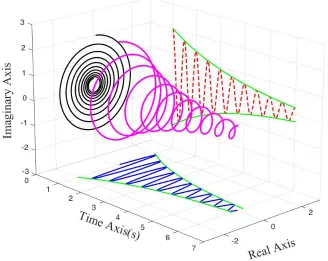
The amplitude above can be considered as the envelope of both real signal and its HT. The original signal is the real part of the analytic signal, and the HT is the imaginary part of the analytic signal. Relationships between original, HT, analytic signal and its envelope can be clearly illustrated by a 3-dimensional representation of analytic signal given in the Figure 1.4. The spiral curve in magenta is the analytic signal in time domain, the real and the imaginary part is simply the projections onto time-real and time-imaginary plane. Similarly, the amplitude is also simply a projection on to the complex plane [2.3].
Figure 1.4. Three-dimensional representation of analytic signal. s+(t)=s(t)+isˆ(t)=3e−
2 5tei(
π 2−4πt)
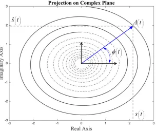
36 The blue solid curve on the Time-Real plane is the original real signal, and the red dash curve on the Time-Imaginary plane is the quadrature pair (HT). The amplitude is added on both real and imaginary part as the green envelope. The black curve on the complex plane (Real-Imaginary) is the projection of the whole analytic signal, and the 𝜙(t) is the instantaneous phase, which is defined as the angle of the analytic signal on the complex plane.
37 Figure 1.6. The analytic signal projected onto the complex plane
38 popular as a tool in transient signal processing. Wu and Huang further introduced a noise-assisted data analysis method, name ensemble empirical mode decomposition (EEMD) in 2009, for solving the mode-mixing problem with the original EMD method, by adding white noise evenly onto the signal during decomposition process [2.4]. With EEMD as the decomposition method, the HHT became more reliable and practical for dealing with signal in the real world.
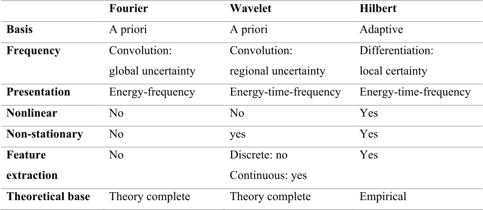
39 Consequently, it has demonstrated that the HHT has a higher resolution in time-frequency domain because of its instantaneous frequency concept, and better computational efficiency than either STFT or WT [2.6][2.7]. A brief comparison is listed in Table 1.2 for better understanding [2.8].
Table 1.2. Comparison between signal processing methods
Fourier Wavelet Hilbert
Basis A priori A priori Adaptive
Frequency Convolution: global uncertainty
Convolution: regional uncertainty
Differentiation: local certainty
Presentation Energy-frequency Energy-time-frequency Energy-time-frequency
Nonlinear No No Yes
Non-stationary No yes Yes
Feature extraction
No Discrete: no
Continuous: yes
Yes
Theoretical base Theory complete Theory complete Empirical
2.1.2. Definition of Hilbert transform in time domain
For a real-valued signal s(t) of one-dimensional real-valued variable t, the Hilbert transform of s(t), a kind of integral transform, is defined for all t as by
(1.36)
and the inverse Hilbert transform is
ˆ s(t)
ˆ
s(t)=H[s(t)]=−1 π
s(τ) t−τ −∞
∞
40
(1.37)
where s(t) and form a Hilbert transform pair.
This integral is improper in the sense that the integrand has a singularity t=τ at and the limits are infinite. This integral in Eq. (2.11) is evaluated as a Cauchy principal value of the integral, whenever this value exists. For simplicity, a symbol P in front of the integral designating the principal value of the integral in most of the books is neglected herein. The Cauchy principal value is then defined as
(1.38)
s(t)=H−1[( ˆs(t)]= 1 π
ˆ s(τ) t−τ
−∞ ∞
∫
dτˆ
s(t)
ˆ
s(t)=H(s(t))= 1
π ε→lim0+
s(τ)
t−τ t−1/ε
t−ε
∫
dτ+ s(τ)t−τ t+ε t+1/ε
∫
dτ⎛ ⎝⎜
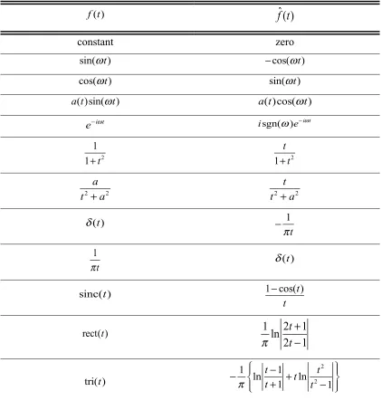
41 2.1.3. Hilbert transform pairs
Some useful Hilbert transform pairs are selected and given in Table 1.3. [2.9][2.10][2.11]
Table 1.3. Selected useful Hilbert transform pairs
constant zero
f(t)
f
ˆ
(t)
sin(ωt) −cos(ωt)
cos(ωt) sin(ωt)
a(t)sin(ωt) a(t)cos(ωt)
e−iωt isgn(ω)e−iωt
1 1+t2
t
1+t2
a
t2+a2
t t2+a2
δ(t) − 1
πt
1
πt δ(t)
sinc(t) 1−cos(t)
t
rect(t) 1
π
ln 2t+1 2t−1tri(t) −π1 ln tt+−11 +tln t
2
t2−1
![Table 1.1. Comparison between LDV and DIC [1.18]](https://thumb-us.123doks.com/thumbv2/123dok_us/1317935.1164554/36.612.79.543.110.388/table-comparison-ldv-dic.webp)