The majority of techniques to determine the minimum water targets based on water pinch analysis (WPA) have assumed freshwater as the sole utility that exists at zero concentration. In practice, regenerated water and externally outsourced water such as rainwater, river water, snow, and imported spent water may exist at varieties of concentrations and can be used to reduce freshwater utility. This paper presents new procedures to establish the minimum flow rate targets for multiple water utilities using the source and sink composite curves. The work offers significant new insights into systematic placement of multiple new utilities through water outsourcing in the context of WPA.
1. Introduction
The advent of water pinch analysis (WPA) as a tool for the design of an optimal water recovery network has been one of the most significant advances in the area of water conservation over the past decade.1-13Water pinch analysis is a systematic
technique for implementing strategies to maximize water reuse and recycling through integration of water-using activities or processes. Maximizing water reuse and recycling can minimize freshwater consumption and wastewater generation.
Typical WPA solution comprises two steps, i.e., setting the minimum freshwater and wastewater flow rate targets followed by network design to achieve the targets. Graphical techniques such as the composite and grand composite curves and numerical techniques such as the problem table14and cascade analysis13
have been used to determine the minimum utility targets and to locate pinch points in heat and water pinch analysis. In pinch heat analysis, the grand composite curve (GCC) has been a well-established tool for multiple utility placement. For WPA, Wang and Smith2have shown that varieties of freshwater sources, such
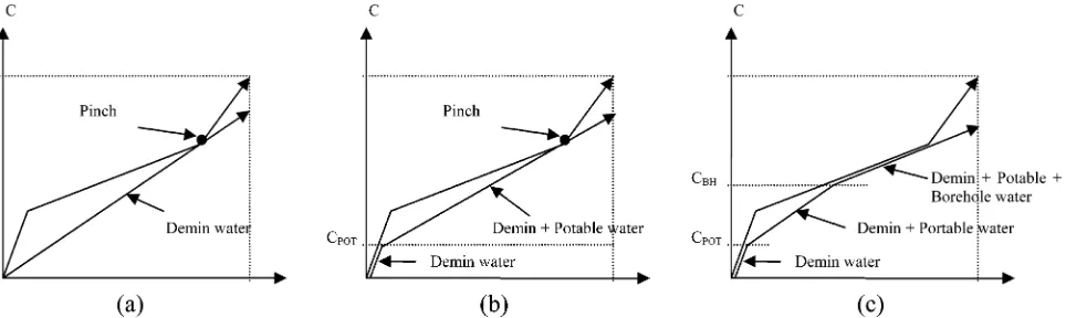
as demineralized water, potable water, and borehole water may be available as utilities, and have used the limiting composite curve (LCC) shown in Figure 1 for placement of multiple water utilities at different concentrations for mass-transfer-based processes. Note that a process may employ either a single or multiple external water sources as utilities at a wide range of concentrations. This “outsourced water” may include rainwater, snow, borehole water, river water, and even “imported” spent water. Other works on multiple utilities targeting were presented by Gomes et al.15using a water source diagram (WSD), Foo16
using water cascade analysis (WCA), and Almutlaq and El-Halwagi17 using algebraic approaches. Other authors have
considered freshwater as the sole water utility, with the vast majority assuming freshwater has zero concentration.
The limiting composite curves and water source diagram, however, are only ideal for cases where water-using processes are modeled as mass-transfer-based (MTB) operations involving
water as a lean stream or a mass separating agent (MSA). In an industrial project where flow rate gains and losses are quite common, it may be necessary to analyze these streams separately and modify the stream data as done by Liu et al.18if the MTB
approach is used. A resilient tool should be able to handle not just MTB but also non-mass-transfer-based (NMTB) water-using operations involving flow rate gain or losses which include water used as a solvent or withdrawn as a product or a byproduct in a chemical reaction, or utilized as heating or cooling media. The water surplus diagram,11 source and sink composite
curves,12and water cascade analysis (WCA) techniques13 fit
the latter category and are well-established alternative methods used recently.
The water surplus diagram11is a grand composite curve used
to target single freshwater utility and wastewater generation in WPA. The surplus diagram is applicable to MTB and NMTB operations and could handle all reuse, recycle, and mixing possibilities. The method, however, involves trial-and-error steps to find the pinch points and water targets and is only suited for targeting freshwater flow rate with zero concentration. El-Halwagi et al.12 proposes source and sink composite curves
(SSCC) as an alternative graphical utility targeting tool that eliminates the trial-and-error steps of surplus diagram and is also applicable to MTB and NMTB processes.
The SSCC is a plot of cumulative contaminant mass load (y-axis) versus cumulative flow rate (x-axis) of sources and demands arranged in ascending order of concentration. The source curve is then shifted along the zero mass load line until a pinch occurs and the source composite curve lies at or on the right of the demand composite curve. For example, the water * To whom correspondence should be addressed. Tel.: +
60(07)-5536049 (S.R.W.A.); +60(07)-5535512 (Z.A.M.). Fax: + 60(07)-5581463 (S.R.W.A., Z.A.M.). E-mail: [email protected] (S.R.W.A.); [email protected] (Z.A.M.).
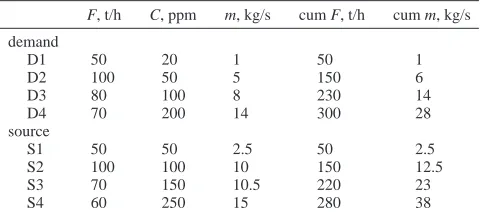
Table 1. Limiting Water Data from Polley and Polley6
F, t/h C, ppm m, kg/s cum F, t/h cum m, kg/s demand
D1 50 20 1 50 1
D2 100 50 5 150 6
D3 80 100 8 230 14
D4 70 200 14 300 28
source
S1 50 50 2.5 50 2.5
S2 100 100 10 150 12.5
S3 70 150 10.5 220 23
S4 60 250 15 280 38
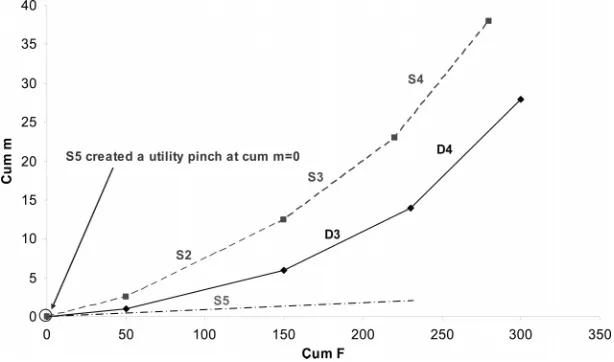
demands and sources from the limiting data in Table 16 are
first plotted beginning at the origin as shown in Figure 2. To get the minimum freshwater and wastewater flow rate targets, the entire source composite is shifted at zero mass load (assuming freshwater has zero concentration) until it touches the demand composite at the pinch point of the water composite curves (in this case, 150 ppm). The horizontal gap between the demand and source composites at zero mass load give the minimum freshwater flow rate (in this case, 70 t/h). The overshoot of the source composite gives the minimum waste-water flow rate (in this case, 50 t/h). The concentration of a stream on an SSCC can be obtained from its gradient. For example, the concentration of S2 shown in Figure 2 is
Kazantzi and El-Halwagi19use SSCC to target a single fresh
utility with nonzero concentration.
Manan et al.13 introduce water cascade analysis (WCA),
which is a numerical version of the NMTB grand composite (surplus diagram) by Hallalle.11WCA allows the designer to
rapidly and accurately generate the minimum water utility targets and water allocation targets, identify pinch-causing streams, and explore options and effects of process changes including regeneration. Foo16recently used the WCA technique to target
multiple utilities. Manan et al.13pointed out that graphical and
numerical approaches are complementary for targeting. A graphical approach is essential as a visualization tool and a numerical approach provides accurate targets.
This paper describes a graphical SSCC procedure to determine the maximum limit for adding multiple water utilities and pure freshwater. This work complements the numerical approaches of Foo16and Almutlaq and El-Halwagi.17The maximum limit
for adding multiple water utilities is referred to in this work as the minimum utility flow rate (FMU). Note that FMUresults in
the minimum freshwater flow rate, FFWU. In this work, FFWU
as a conventional water utility will be clearly distinguished from outsourced utilities (FMU). FMUis an external (outsourced) water
utility with nonzero concentration. FFWU refers to a pure
water, intermediate quality (potable) water, and low quality (borehole) water.
Figure 2. Water composite curves from the limiting data of Polley and Polley.6
CS2)12.5 kg/s-2.5 kg/s
220 t/h-120 t/h ×1000)100 ppm
Figure 3. Gaps in water pinch analysis research related to targeting multiple
freshwater source at 0 ppm concentration. Kazantzi and El-Halwagi19used SSCC to target a single impure fresh source.
However, they did not consider concentration-based problems and cases where both pure fresh (FFWU) and multiple impure
utility sources (FMU) are involved, as covered in this work.
This work offers significant new insights into systematic placement of single and multiple new utilities involving water outsourcing. This work assumes higher quality utilities to be more expensive and should therefore be minimized in favor of lower quality utilities. The method is currently applicable to single-contaminant systems. The new contribution that has emerged from this work is the establishment of a new procedure and a set of new heuristics to use SSCC to determine the minimum flow rate targets for multiple water utilities at various concentrations.
Section 2 describes the systematic technique to determine targets for a single utility and pure freshwater for pinch and threshold problems using source and sink composite curves. Section 3 presents the technique to set targets for multiple new utilities using source and sink composite curves.
2. Targeting the Minimum Flow Rate for a Single Utility Using Water Composite Curves
The current SSCC technique can only target the minimum flow rate for a single utility freshwater (FFWU) which exists at
zero concentration12and nonzero concentration.19This section
explains how the SSCC could be used to determine the FMU
for a single utility and, at the same time, the minimum pure freshwater target (FFWU). The section is divided into pinched
and threshold problems to evaluate different cases.
Pinched Problems. Prior to determining the minimum new
utilities flow rate (FMU), it is important to establish if a utility
is suitable for a given process using the following heuristic: Figure 4. Location of various water sources relative to the utility line S5.
Figure 5. Utility line (S5) creating a utility pinch.
Figure 6. SLA shifted along S5. Final composite curve with minimum
Heuristic 1: Only consider a water source as utility if its
concentration is lower than the concentration of the pinch.
A utility at a concentration higher than the pinch point will only increase wastewater. Say that a water source at a concentration lower than the pinch is available for the limiting data in Table 1. The FMUcan be obtained by systematically
moving the source line above (SLA) along the utility line (U) and the source line below (SLB) until utilities/process pinches are obtained. The U locus is the line with a slope of the utility concentration forming the path along which SLA/SLB is shifted.
Figure 3 illustrates the locations of source lines above (SLA) and below (SLB) and the U. A utility pinch is a pinch point created by a utility line intersecting a demand composite curve. A process pinch, on the other hand, is a pinch point created by the intersection of the source composite curve and demand composite curve.
Systematic shifting of SLA and SLB to get FMUinvolves
two key steps:
1. To target the minimum pure freshwater (FFWU), move the
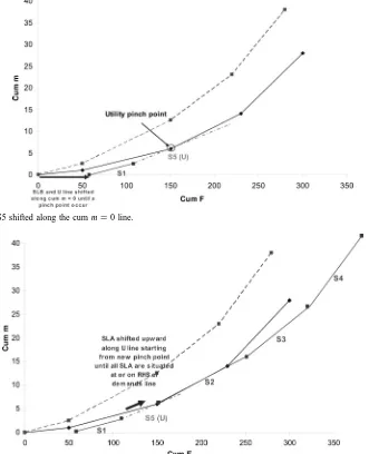
utility line along with SLB to the right-hand side of the demand Figure 7. SLB (S1) and S5 shifted along the cum m)0 line.
Figure 8. SLA (S2-S4) shifted upward along S5 from the new pinch point until SLA created another pinch point at Cpinch)100 ppm.
Table 2. Limiting Data for Example 3
F, t/h C, ppm m, kg/s cum F, t/h cum m, kg/s
demand
D1 10 0 0 10 0
D2 120 5 0.6 130 0.6
D3 50 30 1.5 180 2.1
D4 80 40 3.2 260 5.3
D5 50 50 2.5 310 7.8
D6 30 100 3 340 10.8
D7 90 150 13.5 430 24.3
source
S1 10 10 0.1 10 0.1
S2 70 50 3.5 80 3.6
S3 80 100 8 160 11.6
S4 50 200 10 210 21.6
S5 30 300 9 240 30.6
composite until the line meets either the first utility or process pinch (SLB and utility lines must pinch the demand composite). 2. To target the maximum limit of outsourced utility (FMU),
shift SLA upward along the utility line until the entire SLA pinches the demand composite.
The systematic shifting of SLA and SLB along the U line will be illustrated using four different examples.
(i) Example 1: A utility has no SLB and creates a utility pinch.
S5 at a concentration of 10 ppm is a utility added to the limiting water data from Polley and Polley.6There is no water
source below S5. Hence, the S5 line is drawn first and shifted until a utility pinch (Cpinch) 10 ppm) occurs at cum m) 0
according to step 1 (Figure 4).
SLA (S1-S4) is moved upward according to step 2 along the S5 until a process pinch occurs at Cpinch)150 ppm (Figure
5). The horizontal gap between the demand composite and the intersection of SLA and S5 gives the minimum utility flow rate (FMU), i.e., 75 t/h, and no FFWUis needed. Figure 6 shows the
possible water network design that achieved the target for Example 1. Note that all the designs in this work were produced using the network design guidelines reported by Polley and Polley6and Hallale.11
(ii) Example 2: A utility has an SLB and creates a utility pinch.
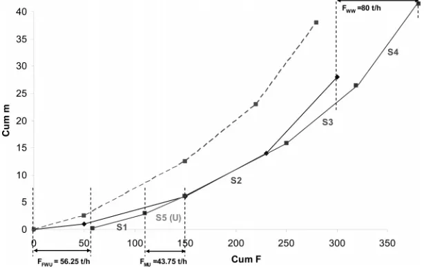
S5 is a utility at 80 ppm added to the limiting data from Polley and Polley.6Shifting SLB (S1) and S5 along the zero “Cum m” axis according to step 1 creates a utility pinch at Cpinch)
80 ppm (Figure 7). SLA (S2-S4) is next shifted according to step 2 along S5 from the new pinch point onward until a process pinch point is created at Cpinch)100 ppm (Figure 8). Figure 9
shows the final composite curves with FMUof 43.75 t/h and FFWUof 56.25 t/h. Figure 10 shows the possible water network design that achieved the target for Example 2.
(iii) Example 3: Utility addition does not create a utility pinch.
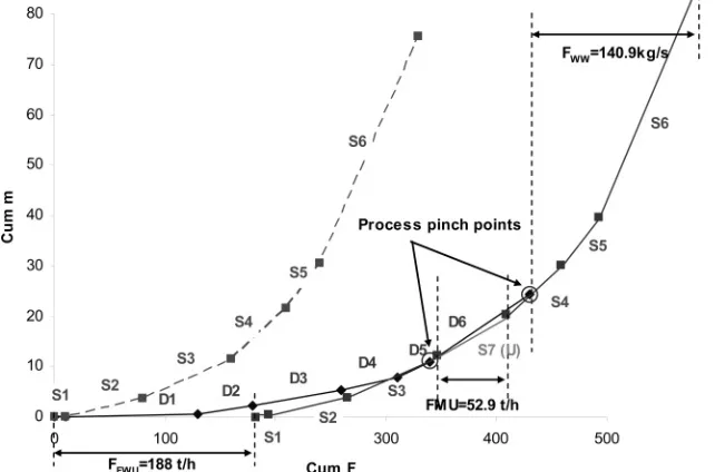
Table 2 shows the limiting data for example 3. S7 is a utility added at 130 ppm. Note that, unlike in the previous examples, shifting S7 and SLB in this case created a process pinch at Cpinch
)100 ppm instead of a utility pinch. Figure 11 shows the final composite curves after shifting S7 and SLB along the zero “Cum
m” axis line and after moving SLA upward from the process
pinch along S7. The FMUfor this case is 52.9 t/h. The process
pinch points are at 100 ppm (on line S3) and 200 ppm (on line S4). The pure freshwater and wastewater targets are 188.0 and
140.9 t/h, respectively. Figure 12 shows the possible water network design that achieved the target for Example 3.
Threshold Problem. A process that has either freshwater or
wastewater as a “utility” is a threshold problem. This example (example 4) focuses on a threshold problem that does not produce wastewater. Foo20 presents the WCA approach for
targeting freshwater for a threshold problem. Next, we dem-onstrate that the graphical SSCC targeting approach can also be applied for threshold problems.
Note that since the flow rate of regenerated source equals the flow rate of reduced wastewater source, regeneration would not change the flow rate of freshwater and wastewater for this case. Harvesting external water source provides more room for savings and is therefore the more preferred option. For this type of threshold problem, a pinch may or may not exist. If a pinch exists, the utility targeting technique for a pinch problem applies. For a threshold problem without a pinch point, the following steps should be taken:
1. Shift the utility line with the SLB until a utility/process pinch point is created.
2. Shift the SLA (S3) above the utility/process pinch point upward along the utility line and the SLB until all demand flow rates are satisfied.
(iv) Example 4: Threshold problem, one new utility (U1) at 80 ppm.
Table 3 is the limiting data for example 4, and Figure 13 is Figure 9. Final composite curves with addition of S5.
the corresponding initial composite curves for a threshold problem. The initial freshwater target is 269.99 t/h. The utility line (S4) at 80 ppm is added and shifted with the SLB (S1 and S2) to the right of the demand composite until a pinch point occurs at Cpinch)80 ppm. The SLA (S3) above the utility pinch
point is shifted upward along the S4 until the water demand flow rates are fully satisfied (see Figure 14). The FMUfor this
case is 50 t/h, and the pinch point is at 80 ppm. The new pure freshwater target is 220 t/h. Figure 15 shows the possible water network design that achieved the target for Example 4. Figure 11. Water composite curves for example 4: a threshold problem.
Figure 12. Composite curves for threshold problem with addition of S4 utility.
Table 3. Limiting Data for Threshold Problem (Example 4)
F, t/h C, ppm m, kg/s cum F, t/h cum m, kg/s
demand
D1 10 0 0 10 0
D2 120 5 0.6 130 0.6
D3 130 10 1.3 260 1.9
D4 50 50 2.5 310 4.4
D5 30 100 3 340 7.4
D6 90 200 18 430 25.4
source
S1 10 10 0.1 10 0.1
S2 70 50 3.5 80 3.6
3. Targeting Multiple FMUValues Using Source and Sink
Composite Curves
Now that we know how to target for a single utilities minimum flow rate (FMU) and a minimum pure freshwater flow
rate (FFWU) using source and sink composite curves (SSCC),
we will proceed to explain how a minimum multiple utility flow rate can be determined.
A higher quality (cleaner) utility is usually more valuable particularly for cases involving regeneration. Thus, when multiple sources of water and regenerated wastewater are available as utilities, the general rule is to minimize the use of
higher quality utility in order to maximize savings. This could be achieved using the following heuristic:
Heuristic 2: Using water composite curVes, obtain the FMU
Values one by one, starting from the cleanest to the dirtiest water
source.
Heuristic 2 means that the FMUfor the cleanest new utility
must be obtained first using the composite curves procedure described Adding a utility will create new utility and process pinch points. The next utility could only be considered if its concentration is lower than the highest pinch concentration. Note that the maximum utility freshwater savings had already been reached with the addition of the first utility. Therefore, addition of a dirtier utility should only reduce the flow rate of the cleaner utility added previously. The same procedure is repeated until all available utilities have been utilized. Example 5 explains how the technique was implemented.
(iv) Example 5: Two new utilities are included: U1 at 10 ppm and U2 at 80 ppm.
To illustrate the technique, the limiting data from Polley and Polley6 are assessed for possible integration with two new
utilities, U1 and U2, available at 10 and 80 ppm, respectively. Note that U1 is S5 from example 1. U1 as the cleaner utility at 10 ppm is considered first according to heuristic 1. Figure 6 shows that the FMU1for S5 is 75 t/h and the utility and process Figure 13. Water composites with addition of U1 (S5) at C)10 ppm.
Figure 14. Shifting of SLB and U2 line (C)80 ppm) along U1 (C)10 ppm) line until a pinch point occurred.
pinches are at 0 and 100 ppm. U2 (S6) at 80 ppm is a viable utility since it existed below the new pinch point at 100 ppm. S6 is drawn next and shifted with SLB (S1) downward along the first utility line (S5) until another utility pinch occurs at 80 ppm (see Figure 16). Next, the SLA above S6, i.e., S2-S4, was drawn at the new utility pinch of 80 ppm and shifted until it completely appeared on the right-hand side of the demand composite, or until it created a new pinch point. This gave FMU1
and FMU2of 64.3 and 35.7 t/h, respectively (Figure 17). The
multiple utility targeting procedures ultimately yielded pure freshwater and wastewater targets at 0 and 79.9 t/h, respectively. Note that if SLA had created a new process pinch when it was shifted along S6, any new water source at concentration lower than the new process pinch point could still be added to further reduce S6. Figure 18 shows the possible water network design that achieved the target for Example 5.
Comparing the results of using two new utilities (Example 5) with the results of using only one new utility (example 1), it can be seen that the former yields the same FFWUtarget as in
the case of only one utility (example 1), i.e., 0 t/h. However, Example 5 achieves FMU1and FMU2values of 64.3 t/h and 35.7
t/h, respectively, whereas example 1 achieves an FMUvalue of
75 t/h. Considering only the total flow rate of the utility, Example 1 clearly yields the better solution. However, since
this work assumes higher-quality utilities to be more expensive, the higher-quality utility should therefore be minimized in favor of lower-quality utilities. The best option, in terms of economy, can be more conclusively determined by conducting a more-detailed economic analysis.
Figure 16. Possible network design for examples 1 and 2.
Figure 17. Possible network design for example 3.
and heuristics have been established to guide the placement of utilities and ensure maximum water savings. The water com-posite curve is the preferred tool as it provides significant insights on how the minimum new utility flow rates (FMU) are
determined and why the reduction occurs.
Nomenclature
Symbols
C)concentration cum)cumulative
D)demand
F)flow rate
t/h)metric tons per hour
m)mass load NU)new utility
P)purity
ppm)parts per million
S)Source
SLA)sources line after new water source line SLB)sources line before new water source line
U)utility
Subscripts
FW)freshwater FWU)freshwater utility max)maximum MU)minimum utility WW)wastewater
Literature Cited
(1) Wang, Y. P.; Smith, R. Wastewater Minimisation. Chem. Eng. Sci. 1994, 49, 981-1006.
Minimization; McGraw-Hill: New York, 1999.
(9) Feng, X.; Seider, W. D. New structure and design method for water networks. Ind. Eng. Chem. Res. 2001, 40, 6140-6146.
(10) Dunn, R. F.; Wenzel, H. Process integration design methods for water conservation and wastewater reduction in industry. Part 1: Design for single contaminant. Clean Prod. Process. 2001, 3, 307-318.
(11) Hallale, N. A new graphical targeting method for water minimi-sation. AdV. EnViron. Res. 2002, 6 (3), 377-390.
(12) El-Halwagi, M. M.; Gabriel, F.; Harrel, D. Rigorous graphical targeting for resource conservation via material reuse/recycle networks. Ind.
Eng. Chem. Res. 2003, 42, 4319-4328.
(13) Manan, Z. A.; Tan, Y. L.; Foo, D. C. Y. Targeting the minimum water flowrate using water cascade analysis technique. AIChE J. 2004, 50 (12), 3169-3183.
(14) Linnhoff, B.; Townsend, D. W.; Boland, D.; Hewitt, G. F.; Thomas, B. E. A.; Guy, A. R.; Marshall, R. H. A User Guide on Process Integration
for the Efficient Use of Energy; Institution of Chemical Engineers: Rugby,
U.K., 1982.
(15) Gomes, J. F. S.; Queiroz, E. M.; Pessoa, F. L. P. Design Procedure for water/wastewater minimization: single contaminant. J. Clean. Prod. 2007, 15, 474-485.
(16) Foo, D. C. Y. Water Cascade Analysis for Single and Multiple Impure Fresh Water Feed. Chem. Eng. Res. Des. 2007, 85 (A8), 1-9.
(17) Almutlaq, A. M.; El-Halwagi, M. M. An Algebraic Targeting Approach to Resource Conservation via Material Recycle/Reuse. Int. J.
EnViron. Pollut. 2007, 29 (1/2/3), 4-18.
(18) Liu, Y. A.; Lucas, B.; Mann, J. Up-to-date Tools for Water-System Optimization. Chem. Eng. Mag. 2004, 1, 30-41.
(19) Kazantzi, V.; El-Halwagi, M. M. Targeting Material Reuse via Property Integration. Chem. Eng. Prog. 2005, 101 (8), 28.
(20) Foo, D. C. Y. Flowrate Targeting for Threshold Problems and Plant-Wide Integration for Water Network Synthesis. J. EnViron. Manage. 2007,
in press. (DOI: 10.1016/j.jenvman.2007.02.007.)
ReceiVed for reView September 21, 2006 ReVised manuscript receiVed June 6, 2007 Accepted June 11, 2007