Copyright2001 by the Genetics Society of America
A Quick Method for Computing Approximate Thresholds
for Quantitative Trait Loci Detection
Hans-Peter Piepho
Institut fuer Nutzpflanzenkunde, Universitaet Kassel, 37213 Witzenhausen, Germany Manuscript received August 26, 1999
Accepted for publication October 6, 2000
ABSTRACT
This article proposes a quick method for computing approximate threshold levels that control the genome-wise type I error rate of tests for quantitative trait locus (QTL) detection in interval mapping (IM) and composite interval mapping (CIM). The procedure is completely general, allowing any population structure to be handled,e.g., BC1, advanced backcross, F2, and advanced intercross lines. Its main advantage is applicability in complex situations where no closed form approximate thresholds are available. Extensive simulations demonstrate that the method works well over a range of situations. Moreover, the method is computationally inexpensive and may thus be used as an alternative to permutation procedures. For given values of the likelihood-ratio (LR)-profile, computations involve just a few seconds on a Pentium PC. Computations are simple to perform, requiring only the values of the LR statistics (or LOD scores) of a QTL scan across the genome as input. For CIM, the window size and the position of cofactors are also needed. For the approximation to work well, it is suggested that scans be performed with a relatively small step size between 1 and 2 cM.
M
APPING of quantitative trait loci (QTL) is of mulas for approximate critical thresholds in BC1and F2 populations, which are applicable in the intermediate growing interest to both breeders and geneticists(Liu 1998;Lynch andWalsh1998; Kaoet al. 1999). map density case. They demonstrated good perfor-mance of these thresholds using simulations (see also QTL mapping procedures such as interval mapping
(IM;LanderandBotstein1989) and composite inter- Doerge andRebaı¨1996). The authors also indicated
that the results ofDavies(1977, 1987) are potentially val mapping (CIM;Jansen1993;Zeng1993, 1994)
in-volve tests of the null hypothesis that a QTL is absent. useful for deriving critical thresholds in other popula-tions and exemplified this for the case of a diallel cross. For a putative QTL position, the likelihood-ratio (LR)
Dupuis (1994) gave another approximation, which in
test statistic asymptotically follows a2-distribution with
simulations by Doerge and Rebaı¨ (1996) has been degrees of freedom equal to the number of associated
shown to be somewhat less accurate than that ofRebaı¨
QTL effects. Since the QTL position is not known,
multi-et al.(1994), leading to slightly inflated type I errors. A ple tests are performed in small steps across the whole
different approach to deriving critical threshold is the genome. To control the genome-wise type I error rate,
permutation test procedure advocated by Churchill
some form of adjustment of the critical threshold value
and Doerge (1994) and Doerge and Churchill
of the test statistic is necessary.LanderandBotstein
(1996). The great advantage of this approach is its con-(1989, 1994) have provided formulas for approximate
ceptual simplicity, its distribution-free nature, and the critical thresholds in IM for a backcross (BC1)
popula-general applicability in different population structures. tion, which are appropriate under the assumption of
A serious drawback is the computational workload. For an infinitely dense map. Feingold et al. (1993)
sug-example, to compute a critical threshold for a genome-gested an approximation, which works well for rather
wise type I error rate of 0.01, at least 10,000 permuta-dense maps (Rebaı¨et al.1994). Further approximations
tions are required to obtain a reasonably accurate esti-for dense (⬍1 cM) and sparse maps are given byDupuis
mate of the threshold (Doerge andRebaı¨ 1996). For
andSiegmund (1999).LanderandBotstein (1989),
a type I error of 0.05, a sample of 1000 permutations is
van Ooijen(1992), andDarvasiet al.(1993) provided
usually regarded as sufficient (ChurchillandDoerge
simulation-based critical values for a number of settings
1994). In routine applications, where many traits need in the intermediate map density case. Using results of
to be analyzed, permutations can pose a formidable
Davies(1977, 1987),Rebaı¨et al.(1994) provided
for-workload.
The purpose of this article is to suggest a quick method to compute approximate threshold values for both IM
Address for correspondence:Institut fuer Nutzpflanzenkunde,
Universi-and CIM using the results ofDavies(1977, 1987). An
taet Kassel, Steinstrasse 19, 37213 Witzenhausen, Germany.
E-mail: [email protected] important aspect of the method is its generality, which
allows any population structure to be handled easily. A need for simulation to compute the approximate thresh-old is not mentioned by Davies (1987), however. In further advantage is computational speed, which is only
of the order of a few seconds, given the LR or LOD fact, his quick procedure requires only very elementary calculations using the values of the test statistic for a profile. The thresholds obtained for real data are
com-pared to those derived by permutation. A simulation is fine grid of positions across the chromosome. Davies did use simulations to verify that his procedure does, conducted to check the appropriateness of the
approxi-mation. in fact, control the type I error rate and has good power. Because of its simplicity and generality, Davies’ quick procedure promises to be very useful for computing THEORY
approximate thresholds for a wide variety of experimen-tal populations such as advanced backcrosses, for which The most common approach to the multiple testing
problem is a Bonferroni adjustment of the significance the more refined approximations are difficult to obtain. In what follows, application of Davies’ quick method to level (Hochberg and Tamhane 1987). When
per-formingMtests, each individual test is assigned a com- IM and CIM is outlined.
Controlling the chromosome-wise error rate:In this
parison-wise significance level of␣/M, which guarantees
the overall type I error rate to be below␣. This method article, it is assumed that QTL are mapped by either IM or CIM using the ML method (Lander and works fine so long as the number of tests is small. In
QTL mapping the number of tests is bounded only by Botstein 1989; Zeng 1994). Thus, LR tests are per-formed across a grid of locations on the chromosome, the step size chosen as we scan across the genome. When
the step size tends to zero, the number of tests (M) so the problem is to find a critical threshold for the LR test statistic that will control the chromosome-wise type approaches infinity, and the Bonferroni approach
breaks down. Essentially this is because correlations I error rate. The proposed method is completely general and not restricted to a particular type of population. among tests at adjacent points on the chromosome are
not exploited. The underlying model assumes a mixture of normal distributions with constant variance and location param-A key to finding a useful procedure is to realize that
in significance testing for QTL, we are in a situation eters depending on the QTL effects. The mixing pro-portions are given by the genotype frequencies and will where a nuisance parameter, i.e., the position of the
QTL, is present only under the alternative hypothesis be specific to the particular population structure under study:
(Rebaı¨et al.1994, 1995). Since the nuisance parameter
is not known even under the alternative, a profile of
T() is the LR test statistic at the putative QTL position the test statistic across the permissible interval for the
in centimorgans; LOD()⫽T()/[2 log(10)]. nuisance parameter is constructed, and we choose the
␣is the chromosome-wise type I error rate. maximum of that profile to perform just one test. Under
Cis the critical threshold value for LR test statistic. the null hypothesis, the nuisance parameter (QTL
posi-kis the number of genetic effects for the putative QTL tion) is undefined, so that standard techniques are not
(kdepends on the population being studied. Exam-applicable for deriving the null distribution of the test
ples: For a backcross population,k⫽1,i.e., one allelic statistic unconditionally on the nuisance parameter. For
substitution effect. For an F2 population,k⫽ 2,i.e., the situation of testing a hypothesis when the nuisance
one additive and one dominance effect). parameter is present only under the alternative,Davies
(1977, 1987) provided an upper bound to the type I It is assumed that T() is a continuous function of, error rate, which is based on the assumption that the except for a finite number of jumps in the first derivative series of tests for different values of the nuisance param- with respect to . A further assumption is that condi-eter form a chi-square process. An evaluation of the tional on the QTL positionT() follows a2-distribution upper bound provides an approximate critical thresh- withkd.f. To detect QTL, the chromosome is scanned
old.Rebaı¨et al.(1994, 1995) found an explicit formula and the maximum of T() is determined over a grid
for the upper bound in case of QTL mapping for a BC1 for [maxT(), say]. The null hypothesis of no QTL and an F2population. The derivations are algebraically on a given chromosome is rejected when maxT()⬎ quite involved, however, even for the simplest case of a C. For a given critical value C, the chromosome-wise BC1population, and extension to other, more complex, type I error rate is bounded above by
designs seems rather complicated.
Davies(1987) had also suggested a “quick calculation ␣ ⫽ Pr(2
k⬎ C)⫹
冦
冮
L0E|
√
T()/|d冧
C (1/2)(k⫺1) of significance” (Equations 2.4 and 3.4) on the basis ofan approximation of his upper bound, which is
consid-⫻ exp
冢
⫺1 2C冣
2⫺(1/2)k/⌫
冢
12k
冣
, (1)ered byRebaı¨et al.(1994) as a useful method for simula-tion-based calculation of the significance value for any
where Pr(2
k⬎C) is the cumulative distribution function experimental design, particularly when an explicit
upper bound in (1) is derived, taking into account the even though only a fraction of points will correspond to real turning points. Thus, to computeV, we simply fact that test statisticsT() computed at adjacent
posi-tionsare stochastically dependent and in fact form a compute the absolute differences between successive square roots ofT() on the grid and sum these across stochastic process. For details of derivation the reader
is referred to Davies (1977, 1987). Note that if we the chromosome.
Davies (1987) notes regarding the one-parameter
dropped the second term on the right-hand side of (1),
Cwould just be the critical value for a conditional test case (k⫽1) that the second term in (3) will be impor-tant whenT() scans across a range of widely differing at a given QTL position. Thus, it can be said that the
second term takes care of the fact that multiple tests hypotheses and then values of T() might tend to be independent for separated values of . This matches are performed and we need to consider theunconditional
distribution of maxT() across the chromosome, rather the situation of a scan across a whole chromosome, where tests⬎50 cM apart are virtually independent. He than the conditional distribution ofT() for a specific
. Thus, the resulting threshold for a prespecified␣will further conjectured that in this case the law of large numbers applies so that V gives a good estimate of be higher than that for the conditional test. Davies
(1987) suggested estimating兰L
0E|
√
T()/|din (1) by 兰L0E|√
T()/|d. His simulations confirmed this con-jecture. From this we expect the approximation to work V⫽冮
L0|
√
T()/|d well for QTL mapping. A small-scale simulation is per-formed to check the appropriateness of the approxima-⫽|√
T(0)⫺√
T(1)|⫹|√
T(1)⫺√
T(2)|tion.
Controlling the genome-wise error rate in IM:To
guar-⫹. . . ⫹|
√
T(r)⫺√
T(L)|, (2)antee a genome-wise type I error rate,Rebaı¨et al.(1994) where1, . . . ,rare the successive turning points (points proposed choosing the same␣ for each chromosome, of inflection) of
√
T(), i.e., the values of , where the using the formula␣i⫽1⫺ (1⫺ ␥)1/n, where␣i is the first derivative
√
T()/changes sign. This change of chromosome-wise error rate for the ith chromosome. sign occurs at the local minima and maxima of This allocation assumes that test statistics for different√
T(). A sign change can (but need not) occur at the chromosomes are stochastically independent, which markers. The advantage of (2) is that it can be computed they are not, since the same phenotypic data are used from the LR (LOD) profile alone, i.e., from the T() for all chromosomes. The effect of dependence will values computed from the data for a grid of values for usually be small, but, nevertheless, we prefer to use the , and does not require further theoretical calculations. Bonferroni inequality (see below), which is guaranteed Using (2) in place of the integral in (1), the upper to control␥, even when the test statistics are dependent. bound of the chromosome-wise type I error rate is esti- A problem for the practitioner is that a separate mated by threshold needs to be used for each chromosome when the same␣iis chosen for each chromosome.Rebaı¨et al. (1994) suggested that␣i“could be chosen by a manner ␣ ⫽ Pr(2k⬎ C)⫹VC(1/2)(k⫺1)exp
冢
⫺ 1 2C冣
2⫺(1/2)k/⌫
冢
12k
冣
. which takes into account the relative lengths of allchro-mosomes.” This suggestion is taken up here. To com-(3)
pute an overall type I error␥, we use the Bonferroni For given ␣, C may be found from (3) by numerical inequality (Hochberg and Tamhane 1987), from methods. The problem in practice is to find the turning which it follows that choosing␣
iso that points 1, . . . , r. In most cases, this will have to be
done numerically. Usually a grid search is done over all
兺
n i⫽1␣i⫽ ␥, (4)
, so the turning points can only be determined to the
accuracy given by the step size of the grid. We therefore where n is the number of chromosomes, will ensure suggest using a relatively fine grid,e.g., between 1 cM that the overall type I error rate is at most␥. Inserting and 2 cM. The analysis is simplified by pretending that the approximation (3) into (4), we find
every point on the grid is a turning point. To see this,
assume that1,2, and3are three successive positions ␥ ⫽nPr(2
k⬎C)⫹
冢
兺
ni⫽1
Vi
冣
C(1/2)(k⫺1) on the chromosome and that T() is monotonicallyincreasing in the interval (1, 3) so that 2 is not a
⫻exp
冢
⫺ 1 2C冣
2⫺(1/2)k/⌫
冢
12k
冣
, (5) turning point. Due to the monotonic increase ofT()we have
where Vi is the value of V for the ith chromosome.
|√T(1)⫺√T(2)|⫹|√T(2)⫺√T(3)|⫽|√T(1)⫺√T(3)|.
Instead of choosing the same␣ifor each chromosome, we suggest that a common critical valueCbe used for It is clear from this result that by pretending that every
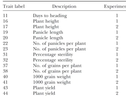
TABLE 1 as bisection,Cis chosen to satisfy (5) for the desired␥.
The resulting chromosome-wise␣ican be inferred from List of rice traits used for QTL mapping (3), though this is not necessary in practice. Assuming (P. Moncada, personal communication) uniform coverage of the genome by markers,␣iwill be
Trait label Description Experimenta
relatively large for longer chromosomes. This seems a perfectly natural allocation of error rates.
11 Days to heading 1
Extension to CIM: In CIM, cofactors are used to re- 16 Plant height 1
duce residual variation by controlling for the genetic 17 Plant height 2 background (Jansen1993;Zeng1993, 1994). Cofactors 19 Panicle length 1
20 Panicle length 2
are determined by model selection procedures such
22 No. of panicles per plant 1
as forward selection and backward elimination. When
23 No. of panicles per plant 2
scanning the chromosome, a certain window size is
im-31 Percentage sterility 1
posed around a putative QTL. Cofactors within the win- 32 Percentage sterility 2 dow are ignored when computing T(). Thus, as we 37 No. of grains per plant 1 scan the chromosome, the set of cofactors changes at 38 No. of grains per plant 2
40 1000 grain weight 1
points bordering the window around the markers used
41 1000 grain weight 2
as cofactors. These points correspond to jumps inT()
43 Plant yield 1
(and its first derivative). The method ofDavies(1987)
44 Plant yield 2
is not directly applicable to CIM because of the
disconti-a1, Monoculture; 2, rice crop following pasture (Brachi-nuities inT().
aria). A simple solution to this problem is to consider in
turn coherent intervals on a chromosome, for which
the same set of cofactors is used in the analysis, so that EXAMPLE T() is continuous within the interval, and to control
We used data from an Oryza sativa ⫻ O. rufipogon the interval-wise type I error rate. The genome-wise type
BC2F2 population evaluated in an upland environment I error rate may then be controlled using a Bonferroni
to exemplify the method and compare it to the permuta-adjustment. Thus, the upper bound for the
genome-tion method. The data were obtained in two experi-wise type I error rate is estimated as
ments, one with rice grown in monoculture and one with rice intercropped with Brachiaria. Details of these ␥ ⫽pPr(2
k⬎C)⫹
冢
兺
pi⫽1
Vi
冣
C(1/2)(k⫺1)experiments are described in Moncada et al. (2000). The traits used for QTL mapping are described in Table 1. IM and CIM results obtained using QTL Cartographer ⫻ exp
冢
⫺ 12C
冣
2⫺(1/2)k/⌫(
k/2), (6)
(Basten et al. 1997) were kindly provided by the
au-thors. The step size of the QTL scans was 2 cM. A step-where p is the number of coherent intervals having a wise selection procedure with aPvalue of 0.01 forF -to-constant set of cofactors. Note that the summation in enter andF-to-drop was used to select cofactors for CIM. the second term on the right-hand side of (6) is over The maximum number of cofactors was fixed at five. thepcoherent intervals. Also, the integration limits in The window size was 10 cM. In permutations for CIM, Viaccording to (2) are now the borders of the coherent the same cofactors were used as those identified in the intervals. Thus, for the border of two adjacent intervals, original analysis. Permutation thresholds at the 0.05 the LR statistic T() has to be computed twice, once significance level were estimated on the basis of 1000 for each of the two intervals, i.e., once with the set of permutations using the procedure ofChurchilland cofactors for the one interval and once with the set of Doerge(1994).
cofactors for the other interval. IM can be regarded as From the output of QTL Cartographer, we did not a limiting case of CIM, in which each chromosome have available the value ofT() at the borders of coher-forms a coherent interval with no cofactors, so thatp⫽ ent intervals. Thus, in computing the sumRp
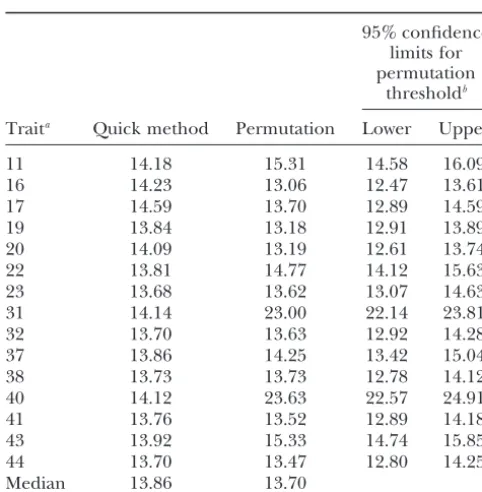
TABLE 2 There is a relatively large variation among permutation thresholds across traits, which cannot be explained by Critical LR threshold values for IM at␥⫽0.05 obtained by
sampling variation alone (see confidence limits), while
permutation (ChurchillandDoerge1994) and by
thresholds computed by the quick method are relatively
the quick method (Davies1987)
stable. The more pronounced variability of permutation 95% confidence thresholds is partly due to the fact that the permutation limits for distribution is unique for each trait, since it is condi-permutation tional on the observed trait values. Thus, some variation
thresholdb
in thresholds is expected, even if all traits are sampled Traita Quick method Permutation Lower Upper from a normal distribution. It should be stressed that despite the larger variation among traits in thresholds
11 14.18 15.31 14.58 16.09
obtained by permutation, it is guaranteed by the theory
16 14.23 13.06 12.47 13.61
of permutation tests (Lehmann1986) that the
proce-17 14.59 13.70 12.89 14.59
dure will control the genome-wise type I error. Both
19 13.84 13.18 12.91 13.89
20 14.09 13.19 12.61 13.74 the permutation procedure and the quick method are 22 13.81 14.77 14.12 15.63 adequate in the case of approximate normality. Note 23 13.68 13.62 13.07 14.63 that differences of thresholds for a particular realized
31 14.14 23.00 22.14 23.81
sample do not imply that over many experiments the
32 13.70 13.63 12.92 14.28
two methods give widely different controls of type I
37 13.86 14.25 13.42 15.04
error. Clearly, any two test procedures may yield
differ-38 13.73 13.73 12.78 14.12
ent results in a specific sample and yet give exactly the
40 14.12 23.63 22.57 24.91
41 13.76 13.52 12.89 14.18 same type I error control over repeated samples, pro-43 13.92 15.33 14.74 15.85 vided the distributional assumptions are met. Traits 31 44 13.70 13.47 12.80 14.25 and 40 have comparatively large permutation
thresh-Median 13.86 13.70
olds. Inspection of the data revealed that for these traits, aFor trait description see Table 1. marked nonnormality and/or presence of outliers were bNinety-five percent confidence interval computed from
a problem. In these cases, the permutation thresholds 937th and 964th order statistic of permutation distribution seem preferable, since the quick method is based on (seeMoodet al.1974).
the normality assumption.
than by permutation, while for CIM the situation is
SIMULATION reversed. By both methods the median threshold is
larger for CIM than for IM. A 95% confidence limit We simulated the chromosome-wise type I error␣for IM in a BC1 population of 200 individuals under the around the permutation threshold was computed using
standard procedures (Mood et al. 1974, Chap. XI). global H0 of no QTL. Equal spacing of markers along
TABLE 3
Critical LR threshold values for CIM at␥⫽0.05 obtained by permutation (Churchill
andDoerge1994) and by the quick method (Davies1987)
95% confidence limits for permutation thresholdb No. of
Traita cofactors Quick method Permutation Lower Upper
11 5 13.99 15.49 14.61 16.23
16 5 14.02 13.52 12.91 13.98
17 5 14.29 14.53 13.75 15.05
19 4 13.93 13.35 12.71 13.93
20 5 14.21 13.32 12.65 14.12
22 5 13.99 14.74 14.25 15.34
23 3 13.64 14.11 13.65 14.83
31 5 14.11 23.24 22.42 24.09
32 5 13.71 14.01 13.51 14.42
Median 14.11 14.74
aFor trait description see Table 1.
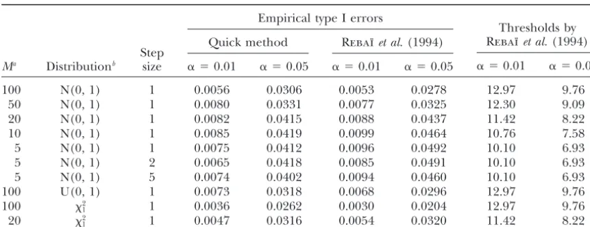
TABLE 4
Simulation of chromosome-wise type I error␣for IM in a BC1population
Empirical type I errors
Quick method Rebaı¨et al.(1994) Step
Ma Distributionb size ␣ ⫽0.01 ␣ ⫽0.05 ␣ ⫽0.01 ␣ ⫽0.05
Thresholds by Rebaı¨et al.(1994)
␣ ⫽0.01 ␣ ⫽0.05
100 N(0, 1) 1 0.0056 0.0306 0.0053 0.0278 12.97 9.76
50 N(0, 1) 1 0.0080 0.0331 0.0077 0.0325 12.30 9.09
20 N(0, 1) 1 0.0082 0.0415 0.0088 0.0437 11.42 8.22
10 N(0, 1) 1 0.0085 0.0419 0.0099 0.0464 10.76 7.58
5 N(0, 1) 1 0.0075 0.0412 0.0096 0.0492 10.10 6.93
5 N(0, 1) 2 0.0065 0.0418 0.0085 0.0491 10.10 6.93
5 N(0, 1) 5 0.0074 0.0402 0.0094 0.0460 10.10 6.93
100 U(0, 1) 1 0.0073 0.0318 0.0068 0.0296 12.97 9.76
100 2
1 1 0.0036 0.0262 0.0030 0.0204 12.97 9.76
20 2
1 1 0.0047 0.0316 0.0054 0.0320 11.42 8.22
Equal spacing of markers is assumed. Simulation is based on 10,000 replications. Length of chromosome⫽ 100 cM.
aM, No. of intervals on a chromosome.
bN(0, 1), standard normal; U(0, 1), uniform;2
1, chi square with 1 d.f.
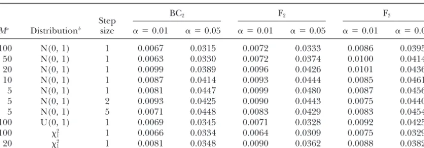
a 100-cM chromosome and absence of interference was by crossing two inbred lines and then proceeding by random mating for several generations. Thus, instead assumed. The number of crossovers per chromosome
was simulated according to a Poisson distribution with of stopping at F2, we continue up to an Ftpopulation. This provides increasing probability of recombination parameter equal to the length of the chromosome in
morgans, which is in accordance with Haldane’s map- and hence increased mapping resolution. We studied an F3 population. The settings (map length, marker ping function. The LR statistic for the null hypothesis
of no QTL was computed using the expectation-maximi- spacing, error distribution, step size, etc.) used for these three types of population (F2, BC2, F3) are the same as for zation (EM) algorithm (LynchandWalsh1998). The
step size was 1 cM in most simulations, but was also BC1. Mapping was done by the EM algorithm assuming absence of interference and Haldane’s mapping func-varied for some simulations to study the effect of step
size. On each of 10,000 simulation runs, we determined tion. The results reported in Table 5 show that the approximation works well across different population the threshold by (5) and checked if H0was rejected at
levels␣ ⫽0.01 and␣ ⫽0.05 anywhere in the genome. types. For comparison, we also assessed the number of
rejec-tions based on thresholds by Rebaı¨ et al. (1994). The
DISCUSSION percentage of rejections was recorded to give an
esti-mate of the actual genome-wise type I error rates (Table This work was motivated by the high computational workload of permutations encountered in practical ap-4). The results indicate that the quick method controls
the type I error, tending to yield slightly more conserva- plications. The method advocated here for computing approximate thresholds is fast and easy to use. Imple-tive thresholds than those ofRebaı¨et al.(1994). Also,
the quick method was rather insensitive to the choice mentation into existing packages for QTL mapping should be possible with minimal effort. Simulations have of step size between 1 and 5 cM. The approximation
performs better for wider marker spacing. For two non- shown that the approximate thresholds provide reason-able, though somewhat conservative, control of the ge-normal distributions (uniform and 2
1), the empirical
type I error was on the conservative side. nome-wise type I error rate in a wide variety of popula-tion structures. Due to the generality of the method, To broaden the scope of the study, simulations were
also performed for an F2population, an advanced back- any population structure can be accommodated. The method is especially useful in more complex designs, cross population (TanksleyandNelson1996), and a
population of advanced intercross lines (AIL;Darvasi where closed form thresholds are not available (ad-vanced backcross, ad(ad-vanced intercross lines, etc.). The
andSoller1995). Advanced backcrossing involves
re-peated backcrossing to one of the parental lines. This rice example has demonstrated that the quick method yields thresholds similar to those obtained by permuta-strategy is especially useful for the discovery and transfer
of valuable QTL alleles from unadapted donor lines into tion. The method is reasonably robust to nonnormality, but should probably be used with caution if departure established elite breeding lines (TanksleyandNelson
TABLE 5
Simulation of chromosome-wise type I error␣by quick method for IM in an advanced backross line (BC2), an F2population, and an advanced intercross population (F3)
BC2 F2 F3
Step
Ma Distributionb size ␣ ⫽0.01 ␣ ⫽0.05 ␣ ⫽0.01 ␣ ⫽0.05 ␣ ⫽0.01 ␣ ⫽0.05
100 N(0, 1) 1 0.0067 0.0315 0.0072 0.0333 0.0086 0.0395
50 N(0, 1) 1 0.0063 0.0330 0.0072 0.0374 0.0100 0.0414
20 N(0, 1) 1 0.0099 0.0389 0.0096 0.0426 0.0101 0.0436
10 N(0, 1) 1 0.0087 0.0414 0.0093 0.0444 0.0085 0.0461
5 N(0, 1) 1 0.0081 0.0447 0.0099 0.0480 0.0087 0.0456
5 N(0, 1) 2 0.0093 0.0425 0.0090 0.0443 0.0075 0.0440
5 N(0, 1) 5 0.0071 0.0448 0.0083 0.0429 0.0083 0.0454
100 U(0, 1) 1 0.0069 0.0345 0.0071 0.0328 0.0092 0.0425
100 2
1 1 0.0066 0.0334 0.0064 0.0309 0.0075 0.0329
20 2
1 1 0.0081 0.0348 0.0090 0.0362 0.0088 0.0382
Equal spacing of markers is assumed. Simulation is based on 10,000 replications. Length of chromosome⫽ 100 cM.
aM, No. of intervals on a chromosome. bN(0, 1), standard normal; U(0, 1), uniform;2
1, chi square with 1 d.f.
replace thresholds obtained by permutation if comput- quick method was robust to nonnormality of errors. Also, in simulations byDoergeandRebaı¨(1996), the ing time is a limiting factor,e.g., when many traits need
to be analyzed. Note that with permutation thresholds, approximate thresholds of Rebaı¨ et al. (1994), which are based on the same upper bound (1) as Davies’ quick the workload increases drastically as the type I error is
reduced, since permutation sample size needs to be method, proved to be relatively insensitive to nonnor-mality.
increased to attain reasonable accuracy. By contrast, the
quick method has the same small workload, regardless Rebaı¨ et al. (1994) have used the quick method of
Davies(1987) to derive simulation-based thresholds for
of the targeted type I error. In summary I recommend
using the quick method preferably in the following situa- the case of F3 progenies derived from a diallel cross between four inbred lines. However, they erroneously tion: (i) a permutation test is computationally too
ex-pensive; (ii) approximate normality can be assumed; assumed that turning points of
√
T() occur only at the and (iii) closed form critical thresholds are not readily marker positions, which is implicit from their Equation available. 10. First, turning points need not occur at the markers. In this article, we have used the maximum-likelihood Second, further turning points will occur at local min-method for computingT(). The method should work ima and maxima of√
T() between markers. For exam-equally well with IM and CIM methods on the basis of ple, in a BC1population, a turning point of√
T() occurs multiple regression (Haley andKnott1992; Marti- whenever the ML estimate of the QTL effect changesnezandCurnow1992). These methods also yield test sign, corresponding to a local minimum. The omission
statistics, which asymptotically follow a 2-distribution
of turning points may explain the liberal thresholds conditional on the putative QTL, so that the theory of obtained byRebaı¨et al.(1994) for their diallel example.
Davies(1977, 1987) applies. The method may also be Furthermore, it does not seem necessary to use
simula-used with IM/CIM on the basis of models that are ex- tions in deriving approximate thresholds. Our simula-tended to account for several random sources of varia- tions indicate that computation ofVfrom the data set tion,e.g., random effects due to genetic correlation and at hand, i.e., not using simulations, gives reasonable, genotype-by-environment interaction (Piepho 2000a). though somewhat conservative, results. Some improve-Moreover, Davies’ method has been used successfully for ment may be possible by using simulations, as suggested marker difference regression (LynchandWalsh1998; byRebaı¨ et al. (1994), though this can no longer be
Piepho2000b), a viable alternative to IM and CIM. called a quick method. Also, if one is prepared to use
When errors follow a normal distribution, the permu- simulation in routine applications, it seems better to tation procedure and the quick method are expected simulate exact thresholds rather than approximate to yield similar thresholds, provided the null hypothesis thresholds. The associated computation costs are the is true. An advantage of permutation tests relative to same and the results are more accurate.
the quick method is that normality of the errors under I thank Pilar Moncada for providing the output from QTL Cartogra-the null hypoCartogra-thesis need not be assumed. Note, how- pher for the rice data. Thanks are also due to Hugh Gauch Jr. for very helpful discussions on the article. This article was written while
Jansen, P. C.,1993 Interval mapping of multiple quantitative trait the author was visiting at the Department of Biometrics, College of
loci. Genetics135:205–211. Agriculture and Life Sciences, Cornell University, Ithaca, New York.
Kao, C. H., Z. B. ZengandR. D. Teasdale,1999 Multiple interval Support of the Heisenberg programme of the Deutsche
Forschungs-mapping for quantitative trait loci. Genetics159:1203–1216. gemeinschaft is thankfully acknowledged.
Lander, E. S.,andD. Botstein,1989 Mapping Mendelian factors underlying quantitative traits using RFLP linkage maps. Genetics
121:185–199.
Lander, E. S.,andD. Botstein,1994 Corrigendum. Genetics136:
LITERATURE CITED 705.
Lehmann, E. C.,1986 Testing Statistical Hypotheses, Edition 2. Wiley, Basten, C. J., B. S. WeirandZ. B. Zeng,1997 QTL Cartographer:
New York. a reference manual and tutorial for QTL mapping. Department
Liu, B. H.,1998 Statistical Genomics.CRC Press, Boca Raton, FL. of Statistics, North Carolina State University, Raleigh, NC. (http://
Lynch, M.,andB. Walsh,1998 Genetics and Analysis of Quantitative
statgen.ncsu.edu/qtlcart/cartographer.html)
Traits.Sinauer, Sunderland, MA. Churchill, G. A.,andR. W. Doerge,1994 Empirical threshold
Martinez, O.,andR. N. Curnow,1992 Estimating the locations values for quantitative trait mapping. Genetics138:963–971.
and the sizes of the effects of quantitative trait loci using flanking Darvasi, A., andM. Soller, 1995 Advanced intercross lines, an
markers. Theor. Appl. Genet.85:480–488. experimental population for fine genetic mapping. Genetics141:
Moncada, P., C. P. Martinez, J. Borrero, M. Chatel, H. G. Gauch 1199–1207.
Jr.et al., 2000 Quantitative trait loci for yield and yield compo-Darvasi, A., A. Weinreb, V. Minke, J. I. WellerandM. Soller, nents in an Oryza sativa ⫻Oryza rufipogon BC2F2 population
1993 Detecting marker-QTL linkage and estimating QTL gene
evaluated in an upland environment. Theor. Appl. Genet. (in effect and map location using a saturated genetic map. Genetics
press).
134:943–951. Mood, A. M., F. A. GraybillandD. C. Boes,1974 Introduction to
Davies, R. B.,1977 Hypothesis testing when a nuisance parameter
the Theory of Statistics.McGraw-Hill, New York.
is present only under the alternative. Biometrika64:247–254. Piepho, H. P.,2000a A mixed-model approach to mapping quantita-Davies, R. B.,1987 Hypothesis testing when a nuisance parameter tive trait loci in barley on the basis of multiple environment data.
is present only under the alternative. Biometrika74:33–43. Genetics156:2043–2050.
Doerge, R. W.,andG. A. Churchill,1996 Permutation tests for Piepho, H. P., 2000b Significance testing for QTL mapping by multiple loci affecting a quantitative character. Genetics142: marker difference regression. Theor. Appl. Genet. (in press).
285–294. Rebaı¨, A., B. GoffinetandB. Mangin,1994 Approximate
thresh-Doerge, R. W.,andA. Rebaı¨,1996 Significance thresholds for QTL olds of interval mapping tests for QTL detection. Genetics138:
interval mapping tests. Heredity76:459–464. 235–240.
Dupuis, J.,1994 Statistical problems associated with mapping com- Rebaı¨, A., B. GoffinetandB. Mangin,1995 Comparing power of plex and quantitative traits from genomic mismatch scanning different methods for QTL detection. Biometrics51:87–99. data. Ph.D. Thesis, Department of Statistics, Stanford University, Tanksley, S. D.,andJ. C. Nelson,1996 Advanced backcross QTL
Stanford, CA. analysis: a method for the simultaneous discovery and transfer
Dupuis, J.,andD. Siegmund,1999 Statistical methods for mapping of valuable QTLs from unadapted germplasm into elite breeding quantitative trait loci from a dense set of markers. Genetics151: lines. Theor. Appl. Genet.92:191–203.
373–386. van Ooijen, J. W.,1992 Accuracy of mapping quantitative trait loci
Feingold, E., P. O. BrownandD. Siegmund,1993 Gaussian models in autogamous species. Theor. Appl. Genet.84:803–811. for genetic linkage analysis using complete high-resolution maps Zeng, Z. B.,1993 Theoretical basis of separation of multiple linked of identity by descent. Am. J. Hum. Genet.53:234–251. gene effects on mapping quantitative trait loci. Proc. Natl. Acad. Haley, C. S.,andS. A. Knott,1992 A simple regression method Sci. USA90:10972–10976.
for mapping quantitative trait loci in line crosses using flanking Zeng, Z. B.,1994 Precision mapping of quantitative trait loci.
Genet-markers. Heredity69:315–324. ics136:1457–1466.
Hochberg, Y.,andA. C. Tamhane,1987 Multiple Comparison