A Study on Selective Ahead-of-Time Compilation for Embedded Java

A

D’MELLO, WARREN JOHN. A Study on Selective Ahead-of-Time Compilation for Embedded

Java. (Under the direction of Dr. Edward F. Gehringer.)

In recent years, Java has been making tremendous inroads into the world of embedded

devices and systems. Thus, it is increasingly important to study the performance characteristics of

the Java Virtual Machines (JVMs), and different optimization strategies that can help boost

application performance.

Usually, embedded systems are very constrained in memory and processor speed, and hence

it is imperative to extract maximum performance without having to incur a high memory cost.

Just-in-time (JIT) compilers give high performance improvements, but they come at a memory

cost (code size, data and code cache requirements) which many embedded systems cannot afford.

A viable alternative is to ahead-of-time (AOT) compile into native code the few hottest – i.e.

most used, most CPU-intensive, and/or time-critical – methods of the application. This results in

a performance boost anywhere from around 88 to 98 percent, while increasing the application

size only marginally.

This thesis presents our research work in performance and analysis of embedded Java

systems. Our work has been divided into two phases. During the first phase, we ran a number of

Java benchmarks on Embedded JVMs. This was mainly to understand the embedded systems, and

their characteristics and performance aspects that made them differ from their desktop

counterparts. The second phase involved executing the aforementioned benchmarks without any

optimization techniques, and then selectively ahead-of-time compiling different methods and

classes of these Java benchmarks and measuring the resulting performance benefits. We

performed an in-depth analysis and study on how to go about profiling the Java application,

selecting the methods that fit the “hot” criteria, AOT-compiling those methods, and subsequently

A

S

S

A

-

-T

C

E

J

By

Warren John D’mello

A thesis submitted to the Graduate Faculty of North Carolina State University

in partial fulfillment of the requirements for the Degree of

Master of Science

Department of Computer Science

Raleigh 2002

Approved by:

_____________________________ _____________________________

D

I would like to sincerely dedicate this thesis to my parents, Bruno and Eleanor D’mello. They

have been my guiding light and have always been there for me. I am the man that I am today

because of their love, hard work, and sacrifice. Words cannot express the gratitude, love, and

respect that I have for them. I can never ever repay you both for all that you have done for me,

and continue to do. Thank you is just a small word in comparison, but that is all that I can say

B

Warren D’mello was born in Bombay, India, and lived most of his life in that beautiful city.

Having achieved his undergraduate degree in Computer Engineering from the University of

Bombay, he decided to gain some professional work experience. He worked for nearly two years

in a multinational Information Technology company, IMRglobal Inc., in Bombay. His job

responsibilities entailed developing client-server applications in Visual Basic, which interfaced

with a variety of databases, such as Oracle, MS SQL Server, and MS Access. During the latter

stages of his employment with that company, he worked on a number of web-development

projects, mainly using Active Server Pages, JavaScript and VBScript. In between, he was sent

overseas for three months, to Sydney, Australia, on a project for Australia Mutual Provident

(AMP). Working for the IT division of the world’s third largest insurance company – Australia’s

largest – was an amazing experience, one never to be forgotten.

Having gained some professional experience, he decided it was time to head back to school

and attain his Master’s degree. During his study, he got a chance to work on a number of

extremely interesting projects, ranging from web-development applications (part-time job with

the nice people at the Crop Science department of NC State, and Dr. Williams’ CSC 591

e-commerce class), Java applications (Dr. Gehringer’s CSC 517 and Dr. Savage’s CSC 505

courses), lower level operating system projects (thanks to Dr. Mueller’s CSC 501 class), and of

course, embedded Java applications (thanks to the good folks at OTI Inc. who gave him so much

advice, support and help). It was thanks to many people, but he must especially mention Dr.

Edward Gehringer, without whom he would never have got such wonderful opportunities.

Now, he looks forward to working here in the US, and gaining some invaluable experience

that will always hold him in good stead. He will always cherish deep in his heart all the memories

A

Words cannot express the gratitude and indebtedness I feel towards Dr. Edward Gehringer.

He has been my mentor throughout these past two years, and has always given me so much of

advice, support and friendship. Without him, this thesis and research work would not have been

possible. He guided me and motivated me, especially when I faltered, never allowing me to doubt

in myself or my capabilities. Thank you so much Dr. Gehringer.

In addition, I would like to sincerely thank Object Technology, Inc. for funding my education

and research work, and for providing me with all the technology and equipment. I would also like

to expressly thank Jim Mickelson, who has been instrumental in guiding and advising me. He has

always been there for me, giving me his invaluable suggestions and comments, which played

such an important role in the accomplishment of this thesis. His unending enthusiasm never

ceased to amaze me, inspite of all my constant questions and doubts. I must have disturbed him

on numerous occasions, especially when this thesis was being drafted, but he still reviewed all

those numerous drafts without even a word of complaint. Thank you Jim; I will never forget all

that you have done for me, and will forever be in your debt.

I am also grateful to Pat Mueller and Scott deDeugd, who arranged for the funding of this

research work, and who assisted me during my course of work. Bruce Hyre, Patrick Dempsey,

Charlie Surface, and Ryan Sciampacone, whose help in setting up the embedded devices and

environments were absolutely invaluable. Tim Wolf and Simon Archer, who helped me

tremendously in my work, and who reviewed a draft of this thesis. DeLoy Bitner and Aldo Eisma

who gave me so much of advice and help in the Ahead-of-Time compilation area. Dave Lavin

and James Branigan, who explained to me the functionality of a few embedded applications.

Andrew Low, for reviewing a draft of this thesis. Finally, my sincere thanks to everybody in the

OTI Raleigh office, for welcoming me with open arms into their wonderful OTI family.

T

C

LIST OF TABLES... vi

LIST OF FIGURES... vii

CHAPTER 1: INTRODUCTION... 1

1.1. Advantages of Java in Embedded Systems... 1

1.2. Considerations in choosing embedded Java... 2

1.3. Thesis Outline ... 4

CHAPTER 2: OPTIMIZATION TECHNIQUES... 5

CHAPTER 3: STUDIES ON CURRENT PLATFORMS... 9

3.1. Platform Configurations... 9

3.2. Embedded Java VMs ... 10

3.3. Existing Java Benchmarks ... 11

CHAPTER 4: INTRODUCTION TO AHEAD-OF-TIME COMPILATION... 16

4.1. Need for Optimization ... 16

4.2. Related Work ... 17

CHAPTER 5: PROFILING THE JAVA APPLICATION... 19

CHAPTER 6: SELECTIVE AHEAD OF TIME COMPILATION... 23

6.1. SmartLinker Options... 23

6.2. Benchmarks and Platforms used for AOT compilation analysis ... 25

6.3. Selective AOT compilation analysis... 26

CHAPTER 7: SUMMARY AND CONCLUSION... 41

Future Research work ... 44

REFERENCES... 45

L

T

L

F

Figure 1: CaffeineMark 3.0, Win NT/x86: No JIT... 12

Figure 2: CaffeineMark 3.0, Win NT/x86: With JIT... 12

Figure 3: SciMark 2.0, Win NT/x86: No JIT ... 13

Figure 4: SciMark 2.0, Win NT/x86: With JIT ... 13

Figure 5: SpecJVM 98, Win NT/x86: No JIT ... 13

Figure 6: SpecJVM98, Win NT/x86: With JIT ... 13

Figure 7: Complete graph of Memory size vs. number of methods AOT’ed - CaffeineMark 3.0 on Neutrino/x86... 28

Figure 8: Partial graph of Memory size vs. number of methods AOT’ed - CaffeineMark 3.0 on Neutrino/x86... 28

Figure 9: Partial graph of Performance vs. number of methods AOT’ed - CaffeineMark 3.0 on Neutrino/x86... 29

Figure 10: Complete graph of Performance vs. number of methods AOT’ed - CaffeineMark 3.0 on Neutrino/x86... 30

Figure 11: AOT analysis of Performance vs. Memory size - CaffeineMark 3.0 on Neutrino/x86... 31

Figure 12: Partial graph of Performance vs. Memory size - CaffeineMark 3.0 on Neutrino/x86 ... 32

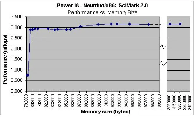
Figure 13: AOT analysis of Performance vs. Memory size - SciMark 2.0 on Neutrino/x86... 36

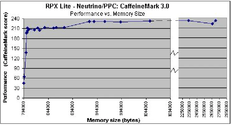
Figure 14: AOT analysis of Performance vs. Memory size - CaffeineMark 3.0 on Neutrino/PPC... 37

Figure 15: AOT analysis of Performance vs. Memory size - SciMark 2.0 on Win NT/x86... 38

Figure 16: AOT analysis of Performance vs. Memory size - CaffeineMark 3.0 on Win NT/x86... 39

Figure 17: Complete graph of Memory size vs. number of methods AOT’ed - CaffeineMark 3.0 on Neutrino/PPC... 46

Figure 18: Partial graph of Memory size vs. number of methods AOT’ed - CaffeineMark 3.0 on Neutrino/PPC... 46

Figure 19: Complete graph of Performance vs. number of methods AOT’ed - CaffeineMark 3.0 on Neutrino/PPC... 47

Figure 20: Partial graph of Performance vs. number of methods AOT’ed - CaffeineMark 3.0 on Neutrino/PPC... 47

Figure 21: Complete graph of Memory size vs. number of methods AOT’ed - SciMark 2.0 on Neutrino/x86 ... 48

Figure 22: Partial graph of Memory size vs. number of methods AOT’ed - SciMark 2.0 on Neutrino/x86 48 Figure 23: Complete graph of Performance vs. number of methods AOT’ed - SciMark 2.0 on Neutrino/x86 ... 49

Figure 24: Partial graph of Performance vs. number of methods AOT’ed - SciMark 2.0 on Neutrino/x86. 49 Figure 25: Complete graph of Memory size vs. number of methods AOT’ed - CaffeineMark 3.0 on Win NT/x86... 50

Figure 26: Partial graph of Memory size vs. number of methods AOT’ed - CaffeineMark 3.0 on Win NT/x86... 50

Figure 27: Complete graph of Performance vs. number of methods AOT’ed - CaffeineMark 3.0 on Win NT/x86... 51

Figure 28: Complete graph of Performance vs. number of methods AOT’ed - CaffeineMark 3.0 on Win NT/x86... 51

Figure 29: Complete graph of Memory size vs. number of methods AOT’ed - SciMark 2.0 on Win NT/x86 ... 52

Figure 30: Partial graph of Memory size vs. number of methods AOT’ed - SciMark 2.0 on Win NT/x86 . 52 Figure 31: Complete graph of Performance vs. number of methods AOT’ed - SciMark 2.0 on Win NT/x86 ... 53

Chapter 1:

I

1.1.

Advantages of Java in Embedded Systems

In recent years, Java has been attracting considerable interest from developers of embedded

systems and devices. Java being highly object oriented (OO), has all the benefits that OO

methodologies have to offer over traditional procedural languages. Java supports multi-threading

inherently, and this results in better responsiveness and real-time behavior. Since Java was

originally intended for use in networked/distributed environments, its capabilities in those areas

are strong and easy to use. This proves useful in embedded devices that have the need to connect

and communicate with other devices. The smaller memory footprint of Java bytecodes, as

compared to applications compiled into native code, presents an attractive option to developers of

embedded devices, where memory size and cost is a crucial issue [4]. Moreover, the inherent

portability characteristics that Java applications possess make them a very viable alternative in

the embedded world, with its myriad of platform configurations. In addition, because of Java’s

in-built safety features, untrusted code can be allowed to execute on devices such as mobile phones,

palm pilots, etc., without the worry of anything malicious occurring. However, it must be kept in

mind that Java applications cannot execute by themselves, and a Java Virtual Machine (JVM) is

needed to interpret and execute the Java bytecodes.

Embedded-system developers have taken an active interest in Java over the past few years,

because the language is abstracted from the underlying hardware, making its applications

portable. With Java, developers can target a particular platform-independent API, and migrate

their applications to different devices without recompiling them [1], unless the application itself

applications can execute from class files containing bytecodes, their memory requirements are far

smaller than that of applications stored in native code.

1.2.

Considerations in choosing embedded Java

A lot of planning and infrastructure is needed to run Java on an embedded device. The

suitability of Java depends on the application and device requirements ― for instance, resource,

integration, and real-time performance requirements [1]. One must also consider the operating

system running on the embedded device. In the embedded world, operating system and hardware

configurations go hand in hand. Moreover, the Java Virtual Machine (VM) that is needed to

execute the Java bytecodes is platform dependent, and not all VMs support the same OS/CPU

combination. A VM that supports a particular OS/CPU combination may not support the same

OS on a different CPU, or the same CPU running a different OS. This was one of the biggest

hurdles that we faced in comparing VMs, since it was very difficult to get more than one VM that

was configured for a particular OS/CPU combination.

In addition, not all the VMs support the same Java specifications, such as, Connected Limited

Device Configuration (CLDC), Mobile Information Device Profile (MIDP), Connected Device

Configuration (CDC), etc. [2], collectively referred to as the Sun Java 2 Micro Edition (J2ME)

specification. This could be due to the fact that the J2ME specification is relatively new. Since

embedded devices can be constrained in memory and CPU performance, and have different

requirements than their desktop peers, it is not practical to have the entire gamut of Sun Java 2

Standard Edition (J2SE) libraries. Instead, embedded JVMs normally follow one or more of the

However, few VMs are yet compliant with any particular J2ME specification or even support

the specification’s libraries. Fortunately, during the past few months, an increasing number of

vendors are moving toward compliance with the Sun J2ME specifications. Moreover, vendors are

developing versions of their VMs to encompass a broader range of OS/CPU combinations.

Finally, one of the biggest questions that embedded system developers face, is the

performance comparisons of embedded Java applications versus those compiled natively.

Admittedly, embedded Java does face a performance drawback against native code since the

application is stored as bytecodes, which have to be interpreted by the Java VM before they can

be executed. This does slow down the execution performance, but not by as much of a margin as

generally presumed. One of the reasons is because the VM technology has been continuously

engineered over the years to optimize and execute the code in the best possible manner. In

addition, it has been shown that in some cases, a well-written Java program could equal or exceed

the efficiency of an average quality C/C++ program [8]. Moreover, just-in-time (JIT) compilers

have been proven to generate extremely efficient and optimized code [3]. In addition, as our

studies and research will show, ahead-of-time (AOT) compilation is another, relatively new,

technique that can be used to increase the performance of embedded Java applications.

These considerations make for a number of decisions when designing and developing

embedded devices. Java hardware manufacturers and software developers have to decide which

hardware configuration to use, whether to use a software VM, accelerator or Java hardware

engine, and if a VM, then which vendor’s VM. To make intelligent decisions, they have to

understand the performance consequences of these different embedded Java solutions for their

applications. Not enough information is currently available for customers and manufacturers to

1.3.

Thesis Outline

In the following chapter, we explain the optimization techniques that are available to

embedded Java application developers. We then go on to describe the results of our work in the

execution of existing benchmarks on a few embedded JVMs, and understanding their

performance shortfalls. We make a short mention about JIT compilers and their performance

advantages, as compared to when the VM simply interprets the application’s bytecodes. We then

go on to describe in detail the study that we conducted on AOT compilation. We start by

discussing how to profile the application in order to find the hot methods and/or classes, and then

natively compile those sets of methods. Finally, we chart the performance gain and memory size

increase as we increase the number of the methods that are AOT-compiled. In conclusion, we

give a few suggestions based on our experience with AOT compiling, and leave a few open

Chapter 2:

O

T

Normally, Java programs are compiled into class files comprising Java bytecodes, which are

machine independent, so that they are not reliant on the underlying hardware configuration.

However, this could cause Java to take a performance hit, since these bytecodes have to be

translated to machine code at run time. To overcome this, numerous Java vendors opt for

solutions such as just-in-time compilation (JIT) [4, 5], ahead-of-time compilation (AOT) [8, 9,

11, 12], or even hardware systems that directly execute the bytecodes [6].

The most common technique is an intelligent JIT, wherein the bytecodes are dynamically

translated/compiled into native code, which is then executed directly. We say here intelligent JIT

because when JIT technology was still in its infancy, some JIT implementations used to translate

every method of the Java application [4]. This used to cause quite a big memory overhead for

storing all the compiled native code in the JIT compiler’s code cache, since the cache was usually

a primitive queue (most likely FIFO), and methods could get replaced quite often. This was not

too consequential in desktop/server environments, where memory was not a scarce resource.

However, when small, memory-constrained, embedded environments were considered, memory

overhead became crucial. Hence, today, most vendors use more intelligent JIT systems, which

analyze the application at run time, and decide which compiled methods should be stored in its

cache memory for future use [5]. The JIT makes these decisions based mainly on the number of

times the method is called, after which it has to compile the method and save the resulting native

code in its cache. This number can be specified and tuned in most modern VMs. In addition,

advanced JIT compilers use runtime profiling and adaptive re-compilation techniques. Moreover,

developer to vary the level of optimization, from a fast JIT (less optimization) but slower

application, to a slower JIT (more optimization) but faster application.

Hence, developers must consider the tradeoffs between memory size and performance.

Depending on the CPU instruction set, the size of the application code expands as it is compiled

from bytecodes to machine code. Typically, we have observed that the expansion ranges from

three to ten times. Thus, more memory is required for the JIT cache as one increases the number

of methods to save. Moreover, a JIT may not be appropriate for some applications or platforms ―

for instance, if performance already meets expectations and the developers do not want the

additional complexity of a JIT compiler in their device. Or, in some cases, developers may not be

able to afford the additional memory overhead of a JIT compiler that is needed for the JIT code

itself, as well as the code cache that the JIT uses to store the compiled methods. In this case, they

may prefer to sacrifice performance instead of the incurring the cost for the additional memory.

Embedded application developers thus have great flexibility in tuning their applications and

hardware environments.

Where performance is more critical than memory, developers could opt to ahead-of-time

(AOT) compile the entire Java application [8, 9]. The application will certainly be larger than

with Java bytecodes, typically an order of magnitude expansion, as mentioned earlier, but

performance will be better. However, advanced VMs and their accompanying integrated

development environments (IDEs) allow developers to AOT-compile specific classes or methods.

For instance, CPU-intensive or time-critical methods, termed hot methods, may be compiled

ahead of time, while the rest of the application remain in bytecode. Thus, selective AOT

compilation allows the size of an application to be traded off against performance. It may allow a

methods does require quite a detailed performance analysis of the Java application. Fortunately,

advanced tools are available to aid in this analysis, as we will describe in subsequent chapters.

It must be noted here that AOT compilation is different from compiled Java. In the latter

case, there is no need for having a VM, and the Java application is compiled into machine code

and run as an executable. In case of the former, we still have the VM, along with the

AOT-specific shared object files that are needed for relocation support, native support, garbage

collection, and exception-throwing support. Moreover, since only certain specific methods are

AOT-compiled, the resulting application is a mix of bytecodes and native code. The VM handles

the transition between these different types of code formats, and allocates memory and fixes the

addresses and values such as constant pool entries, static fields, and class addresses, to name a

few.

In addition to JIT and AOT techniques, developers may use hardware Java processors and

accelerators to improve performance. Java hardware processors that directly execute the Java

bytecodes eliminate the need for an interpreter or JIT, hence avoiding the performance hit of

translating bytecodes into native code [4, 6, 7, 10]. While this seems like an attractive alternative,

it does curtail the developer’s flexibility, since only Java applications will run on these embedded

devices, precluding applications written in popular languages like C. Moreover, device drivers

would have to be written, and hardware accessed, in Java, instead of in C code accessed via the

Java Native Interface (JNI). In addition, since the Java processor directly executes the bytecodes,

the translator is not able to optimize machine code as a JIT compiler would. Another option is for

a Java hardware accelerator, such as a coprocessor, to translate the byte code to native code [6,

10]. So in this case, while a VM is required, a JIT compiler is not needed. However, coprocessors

families. Moreover, the cost of these hardware solutions is quite exorbitant, and this presents a

very real obstacle to embedded system manufacturers who have to mass-produce their devices.

In summary, while there are numerous optimization options available to embedded Java

developers, the final choice rests with the exact needs of the application, as well as the clients and

customers for whom these embedded devices and applications are being developed. Some

applications may not need a maximum performance, as long as their real-time deadlines are met.

Moreover, not many customers may be willing to bear the additional memory cost needed to

achieve a large performance gain. In contrast, some customers may demand maximum

performance at any cost. If memory cost is not a problem, then a JIT could be very suitable, but if

Chapter 3:

S

C

P

During the initial phase of our research work, a number of embedded Java virtual machines

were benchmarked and analyzed on different operating systems (OS) / hardware configurations.

3.1.

Platform Configurations

The VMs were analyzed on the following OS/hardware platforms –

• Microsoft Windows™ NT/x86

• QNX Neutrino™/Power PC

• aJile’s JEM2 processor (Java microprocessor ) [6]

• QNX Neutrino™/x86

The Windows NT environment was included because although it isn’t an embedded

environment, it is used as the reference platform of choice for evaluating and studying different

VMs. Though the conclusions derived from the benchmark studies on this platform may not

reflect all of the characteristics of the VMs in a true embedded environment, they still serve to

give a general idea of how the VMs perform when compared with each other, and how they

behave when memory and resources are not that big a factor. As we mentioned earlier, it is quite

difficult to obtain versions of the VMs from the different vendors that support the same

OS/hardware configuration. One of the reasons for this is that unlike desktop systems, there are

many OS/hardware combinations available for embedded systems and there is no standard

reference platform. Another reason could also be a strategic one, with VM vendors forming

alliances with OS/hardware vendors. In addition, it could also be that the need never arose for a

vendor of a particular VM to develop a version for a given OS/hardware platform. Nonetheless,

parameters of the NT/x86 platform used for the benchmarks are – Gateway desktop PC,

Microsoft Windows NT v. 4, Intel Pentium III 550MHz, and 128MB RAM.

The second platform on which the analysis was performed was a Power PC embedded device

(RPX Lite™) from Embedded Planet. It has a Motorola Power PC 823(e) processor running at

66MHz, with 16MB Flash, 16MB RAM, and 128KB NVRAM. The operating system loaded on

it is QNX Neutrino v. 2.0. This is a true embedded device, but unfortunately, only one VM

(IBM’s VAME) could be analyzed on this configuration, since no other VM supported this

OS/CPU combination.

The third platform that has been studied deviates quite a bit from the previous two platforms.

It consists of a microprocessor that directly executes the Java bytecodes, and therefore an

interpreter/JIT is no longer needed to execute the Java application. The embedded device used in

the study was an evaluation board, aJ-PC104 system from aJile, which had a JEM2 direct

execution Java microprocessor running at a 40MHz, with 1MB SRAM, and 1MB Flash.

The final configuration that was studied only during the second phase, when we conducted

our AOT analysis, was an advanced embedded board from CP Technology, named Power IA

Service Gateway. It contained a 233MHz National Semiconductor x86 chip, along with 32MB

Flash, and 128 MB RAM. The operating system loaded was QNX Neutrino v. 6.1.0.

3.2.

Embedded Java VMs

The Embedded Java VMs/processor that were considered in the study are –

• aJile JEM chip, aJile Systems

• PersonalJava 3.1, Sun Microsystems

• Jeode 1.7, Insignia

• VisualAge Micro Edition (VAME) 1.3, IBM

• WebSphere Studio Device Developer (WSDD) 4.0, IBM

Since we studied the WSDD VM only during the second phase of our research, the results for

it will be discussed only in the subsequent chapters.

3.3.

Existing Java Benchmarks

We considered three benchmarks for our studies, namely –

• Embedded Caffeine Mark 2.0™

• SciMark 2.0™

• SPECjvm98™

Embedded Caffeine Mark 3.0 from Pendragon Software

(http://www.pendragon-software.com/pendragon/cm3/) is very widely used for benchmarking and comparing Java VMs.

It contains numerous tests such as Sieve of Eratosthenes, for finding prime numbers, sorting and

sequence generation, decision-making instructions, recursive function calls, and floating-point

tests that simulate 3D rotation of objects around a point. The scores are based on CaffeineMark’s

own scale.

The SciMark 2.0 test from the National Institute of Standards and Technology (NIST) is a

mathematically intensive test that tests the VMs’ performance in a number of mathematical

algorithms such as Fast Fourier Transform, Jacobi Successive Over-Relaxation, Monte Carlo

mflops (million of floating point operations per second). More information about this test can be

found at http://math.nist.gov/scimark2/about.html

SPECjvm 98 was the final benchmark used during the first phase of our analysis. Developed

by SPEC, it is recognized industry-wide as the most demanding Java VM benchmark. It contains

eight benchmark programs that conduct array-indexing tests, method calls, Lempel-Ziv

compression, Java Expert Shell System, multiple database functions, Java code compiling,

operations on audio files, ray-tracing, and a Java parser generator. However, this benchmark,

being large as well as very intensive and demanding, is not suitable for running on embedded

devices, and hence was not used in the second phase. It served mainly as a performance

comparison between the different Java VMs. Detailed information about this benchmark can be

found at http://www.spec.org/osg/jvm98/jvm98/doc/benchmarks/index.html

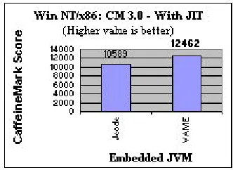
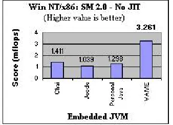
A summary of the benchmark results is displayed in the following figures and tables. Figures

1 through 6 display the benchmarking results for the different VMs on the Windows NT/x86

platforms. It can be clearly observed that using a JIT yields about a ten-fold increase in the

performance of the VM.

Unfortunately, at the time of the comparisons, Sun’s PersonalJava did not have any JIT

support, nor were we able to obtain a copy of the JIT version of HP’s Chai (TurboChai). Hence,

we could not perform any JIT analysis on those JVMs.

Figure 3: SciMark 2.0, Win NT/x86: No JIT Figure 4: SciMark 2.0, Win NT/x86: With JIT

For certain applications such as some of the SPEC benchmarks1_{, the default stack size was}

not sufficient to run the benchmark, and had to be increased manually via the command line.

Figure 5: SpecJVM 98, Win NT/x86: No JIT Figure 6: SpecJVM98, Win NT/x86: With JIT

In addition, while the IBM VM does very well in the SPEC and CaffeineMark benchmarks

(Figures 1, 2, 5, and 6), which are more generalized benchmarks, Insignia’s Jeode seems to do

slightly better in the mathematically focused SciMark benchmark, only with the JIT compiler

switched on, as can be seen in Figure 4. While it is debatable whether in-depth mathematical

operations are typical of embedded applications, the benchmarks do indicate the strengths and

weaknesses of different VMs.

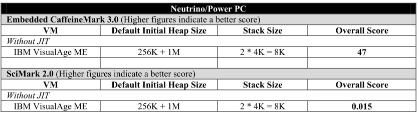
Table 1 shows results from the benchmarks that were conducted on an embedded device,

namely, the RPX Lite from Embedded Planet.

Table 1: Neutrino/Power PC VM performance results

Neutrino/Power PC Embedded CaffeineMark 3.0 (Higher figures indicate a better score)

VM Default Initial Heap Size Stack Size Overall Score

Without JIT

IBM VisualAge ME 256K + 1M 2 * 4K = 8K 47

SciMark 2.0 (Higher figures indicate a better score)

VM Default Initial Heap Size Stack Size Overall Score

Without JIT

IBM VisualAge ME 256K + 1M 2 * 4K = 8K 0.015

Since the IBM VM was the only VM available that runs on a Neutrino/Power PC platform, a

proper comparison against other VMs could not be performed. However, these figures clearly

show the differences between the desktop and embedded worlds. In the desktop environment,

resources such as memory and CPU speed are plentiful, and the VMs can execute very quickly.

However, in the embedded world, the VMs can be faced with such constrained environments and

resources, that there is a clear difference in the execution speeds of the benchmarks. Two points

should be noted here. One, the IBM VAME 1.3 version did not have JIT support for the

Neutrino/Power PC platform, and hence there are no results for the benchmarks with the JIT

turned on in this platform. The latest version, 1.5 (WSDD 4.0), does however have JIT support

for this platform, and those results are displayed in the subsequent chapters. Secondly, as

mentioned earlier, we were not able to execute the SPEC benchmark on this Neutrino platform. It

is primarily a desktop/server benchmark, and the Neutrino/Power PC embedded environment had

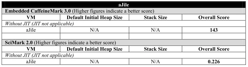
In Table 2, we observe the results of running two of the benchmarks, namely CaffeineMark

and SciMark on the aJile JEM2 processor. In this case, though we cannot make a direct

comparison between these results and those of the software VM that was used in the

Neutrino/Power PC embedded environment, we do get an estimate of how the Java

microprocessor stacks up against the software VMs.

Table 2: aJile JEM2 Java microprocessor performance results

aJile

Embedded CaffeineMark 3.0 (Higher figures indicate a better score)

VM Default Initial Heap Size Stack Size Overall Score

Without JIT (JIT not applicable)

aJile N/A N/A 143

SciMark 2.0 (Higher figures indicate a better score)

VM Default Initial Heap Size Stack Size Overall Score

Without JIT (JIT not applicable)

aJile N/A N/A 0.226

However, we must keep in mind the costs of choosing a hardware Java solution over a

software VM (see Chapter 2.) To reinforce this point, we must mention here that we had to

customize one of the benchmarks a bit in order to enable it to run on the aJile Java processor

evaluation board. No change was made in the benchmarking processes themselves, but in the way

the benchmark application handled the parsing of the command-line parameters. Moreover, the

benchmarks had to run under the supervision of one of the software environments that

accompanied the board. This environment presumably handled memory allocation and thread

creation for the Java processor, and displayed the standard input/output on a console screen.

To summarize, we conducted a performance analysis of different embedded Java virtual

machines (JVMs) on different platforms. This enabled us to gain an understanding about

embedded Java VMs, and their execution in embedded environments. We were able to study the

Chapter 4:

I

A

-

-T

C

4.1.

Need for Optimization

The nature of embedded devices presents some imperatives that must be met. The footprint

must be kept small because memory resources, such as RAM and ROM, cost money. Many

devices respond to outside stimuli and need to react quickly, or within a fixed deadline; therefore,

performance has to remain high. Behavior must be robust and predictable, as users will not put up

with anything less. A number of applications have to be flexible and dynamically upgradable,

ideally over the net. The very nature of the emerging connected world is what is pulling Java into

embedded devices [10], because, as mentioned earlier, Java is well suited for use in networked

and distributed environments.

A typical Java system usually includes the application, Java class libraries, the Java Virtual

Machine (JVM), and often, a set of native applications or libraries. The challenge in embedded

systems is to find the size, cost, and/or performance tradeoff between these elements. While

speed, size, and predictability are interrelated, one major performance issue is the nature of Java

as an interpreted language [10]. Although Java in interesting in its own right, one factor for its

popularity stems from its “write once, run anywhere” ideal. Java's mobility is achieved by

compiling its object classes into a distribution format called a class file. A class file contains

information about the Java class, including bytecodes, an architecturally neutral representation of

the instructions associated with the class’ methods. A class file can execute on any

computer/device supporting the Java Virtual Machine. Java's code portability, therefore, depends

on both architecture-neutral class files, and the implicit assumption that the JVM is supported on

Most JVM implementations execute bytecodes via interpretation, or just-in-time (JIT)

compilation, which compiles the bytecodes into machine code at run-time. Thus, Java's

portability comes at the price of interpreting or JIT-compiling the bytecodes every time the

program is executed. These systems incur modest to severe performance penalties, as compared

to more traditional systems that compile source code directly to machine code only once. For

example, a compiled C program runs 1.5 - 2.2 times faster than the equivalent JIT-compiled Java

program and 2.6 - 4.2 times faster than an interpreted Java program [9].

Now, a number of embedded applications are real-time and cannot afford to have their

deadlines missed. They do not need to have super-fast performance, as long as their deadlines are

met. Alternatively, there are some applications that just need to be extremely fast. In both cases,

increasing the device’s resource capabilities, such as CPU speed and/or memory size, may not be

a viable option. It must be understood that most often, these embedded devices are

mass-produced; even a small increase in cost per device could result into a huge expense. This is where

we feel that our study in selective ahead-of-time compilation could prove extremely beneficial.

4.2.

Related Work

Ahead-of-time compilation is a relatively new technique that is being applied to embedded

Java applications. Most of the previous studies and articles [9, 10] have discussed AOT compiling

the entire Java application. These studies mainly apply to the desktop environment, and are

definitely not feasible in the embedded world where the constrained memory cannot support the

size of the entire natively compiled Java application. In our research work, we do not natively

compile the entire application, but only those methods and/or classes that fit the hot criteria. We

We have come across a few studies that are related to our work. The first one – Matthew

Arnold et al [11], confirms our view that sample-based profiling is accurate enough for the

methods that matter. It is not as invasive as time-based profiling which perturbs the code.

However, this study mainly considered optimizing the code of the hot methods, and not natively

compiling them as we have suggested in our research. Moreover, their study is mainly related to

desktop environments and not embedded systems per se.

The second study, conducted by Aldo Eisma [12], is very much related to our work on

ahead-of-time compilation for embedded Java systems. However, his paper talks about using an

automated tool to find the hot methods, and natively compile them according to set criteria of

desired performance gain. Our research is centered mainly on manually profiling the Java

application, studying the profile output to obtain the hot methods, and then natively compiling

those methods according to the desired level of performance gain and memory usage. We feel

that our work will enable the embedded developer to have a tighter control over which methods

are AOT-compiled, allowing him to fine-tune it according to his criteria. The developer will have

more visibility into the tradeoffs between performance gain and memory cost, and this will assist

Chapter 5:

P

J

A

The first step in selectively ahead-of-time compiling a Java application is to profile it; that is,

analyze the application’s performance and find the methods where it is spending most of its time.

This enables us to find out which methods are the most used, and/or which are most

CPU-intensive (these are the criteria for being “hot”). There are quite a few tools available to profile

Java applications, but the one we used was the IBM SmartLinker™ Profiler. This tool is provided

along with the IBM WebSphere™ Studio Device Developer (WSDD) 4.0 IDE.

Once the application is imported into the IDE, then one can profile it either locally – on the

development machine – or remotely, on the target device. If the developer opts for the latter, then

certain hooks – lines of code, must be inserted in the application, at the appropriate areas that

need to be profiled. We chose the former option, since theoretically, the methods that are hot in

the development environment, should be the same in the embedded device. This was later verified

by our findings; since we obtained similar performance curves across all the three platforms that

we ran our tests on.

Once it has been decided to profile the application locally, the next step is to specify a

number of different options to the SmartLinker. One of the first options is the type of output

format that the Profiler will generate. There are two types of formats, Extensible Markup

Language (XML), and Comma Separated Values (CSV). The former is suitable for interfacing

with other tools. For example, it is used by the SmartLinker tool in the feedback-directed AOT

compilation [12], to automatically select the methods that are to be AOT-compiled, in order to

do a bit of research on the automatic feedback-directed AOT compilation, we found that it did not

give us the granularity and level of control that we had with manual AOT compilation. Moreover,

we observed that performance was not congruent with what it should have been. Therefore, we

feel that a manual analysis, though a little more painstaking, provides slightly better results, with

a finer control over memory usage and performance gain. This allows for better analysis of the

tradeoffs between memory and performance. Finally, the automatic feedback-directed AOT

compilation is specific to only one tool, namely, the IBM SmartLinker™ Profiler. Our research is

more generalized and can be implemented using other tool sets. All that is needed is a profiler, to

analyze the Java application; a compiler, which can AOT-compile the specified methods and/or

classes; and a runtime VM, which can support a mixed format of methods – bytecodes and

AOT-compiled.

The next option that is available is whether to profile the application using a sample-based

technique or instrumented profiling. As we mentioned earlier, it has been shown that a

sample-based profiling is sufficient for finding the hot methods [11]. The sampling method is efficient,

although it is fairly coarse-grained, and considering the processor speed, the sampled profile is

likely to contain some imprecision. This is especially true for short-running applications.

However, the time-based profiling is also imprecise, since, as is mentioned in the study by Arnold

et al., the instrumentation introduces overhead, increases code size, and disrupts the instruction

cache. They showed that the sample-based profiling is no worse than time-based, and at times,

even better. Therefore, it is possible that the hot methods obtained by the sample-based profile are

more accurate than those obtained by the time-based profile. Due to all these reasons, we elected

to use sample-based profiling in our research, and this proved to be sufficient and accurate

enough, as our forthcoming results will demonstrate. It must be noted that in either case, the

profiling tool is invasive, and the application’s performance, be it a benchmark score or time

The SmartLinker Profiler provides an option to specify either to profile from the start, or only

certain areas of the application. In the latter case, the developer will have to insert certain lines of

code – hooks, as we mentioned earlier, before and after the areas to be profiled. This is especially

good if the developer suspects certain problematic areas in the application, and needs to see how

long those areas take to execute. In our case, we profile the entire application, from the start until

the end, in order to obtain all the hot methods. This gives us an exact idea as to which methods

are the most CPU intensive, and which methods are called the most number of times (most used).

Finally, once all the options have been set, the application is executed, with the SmartLinker

Profiler taking samples at regular intervals. The duration of the intervals depends on the operating

system that is being used. Windows NT™ has a minimum granularity of 10 milliseconds (ms),

while real-time operating systems like QNX Neutrino™ have a much finer granularity,2 _{and the}

tool can profile as low as 1 ms on these systems. For the two applications that we considered in

our analysis, 10 ms seemed to suffice. One reason was that the profile output was nearly the same

across multiple profile runs. The second reason that confirmed our view was that the time-based

profiling output was similar to that of the sample-based profiling for the top ten percent of the hot

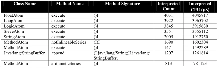
methods. Once the application has completed executing, the Profiler will generate the output

profile file (CSV file in our case). This output contains a number of columns – Class Name,

Method Name, Method Signature, Interpreted Count, Interpreted CPU, to name a few. The

Interpreted Count column indicates how many times the method was interpreted, that is, how

many times during each sampling of the application, the method was found to be executing. The

Interpreted CPU column indicates the total time, in microseconds (µs), that the method took to

execute, across all the counts. We import this CSV file into a spreadsheet, and then sort the data

on these two keys, Interpreted CPU and Interpreted Count respectively, in descending order. The

top methods then obtained are the hottest methods. A partial sample of the sorted output is

displayed in Table 3.

Table 3: Sample sorted Profiler output (CSV format) for the CaffeineMark benchmark

Class Name Method Name Method Signature Interpreted

Count Interpreted _{CPU (µs)}

FloatAtom execute ()I 4031 4045817

LoopAtom execute ()I 3922 3965702

LogicAtom execute ()I 3845 3915630

SieveAtom execute ()I 3551 3555112

StringAtom execute ()I 2005 1912750

MethodAtom notInlineableSeries (I)I 1690 1602304

MethodAtom execute ()I 1471 1592289

Java/lang/StringBuffer append (Ljava/lang/String;)Ljava/lang/

StringBuffer; 1207 1261814

MethodAtom arithmeticSeries ()I 813 781123

As can be observed, the FloatAtom.execute()I method is the hottest method, followed by

the LoopAtom.execute()I, and so on. Note that the complete method signature is comprised

of the Class name, method name, and parameter/return value types (displayed under the Method

Signature column of the table above).

Therefore, by profiling the application and then sorting the resulting profile output, we were

able to obtain the most used and/or most CPU intensive methods. Having obtained these hot

methods, the next step is to ahead-of-time compile these methods. The subsequent chapter

describes in detail the steps involved in ahead-of-time compiling these methods, and then

Chapter 6:

S

A

T

C

6.1.

SmartLinker Options

Once the profile output has been obtained and sorted, the next step is to natively-compile the

top few methods, i.e., the hot methods. We used the IBM SmartLinker tool to natively-compile

the methods. In a typical embedded application build scenario, the embedded targets cannot

easily be used to build the application. The applications are built on development workstations,

using cross-compilers, which compile the application on one platform for execution on another

platform. The SmartLinker tool, which accompanies the WebSphere Studio Device Developer

(WSDD) 4.0 IDE, can currently compile for different operating systems (OS), but only across the

same CPU family.3 _{For instance, it is possible to generate code for a Neutrino/x86 platform on the}

Windows NT/x86 platform itself. However, in order to compile code for the Neutrino/PPC

embedded platform, one would need a PPC platform that has larger memory resources and CPU

speed, such as Neutrino or AIX desktops.

Hence, one of the AOT-compile options in the SmartLinker tool is the specification of the

hardware and OS platform for which to generate the code – for example, “ia32- windows” for

Windows/x86, “ia32- neutrino” for QNX Neutrino/PPC, aix” for AIX/PPC, and

“ppc-neutrino” for Neutrino/PPC, to name a few. In our research, we used the Windows NT/x86

desktop to build for the x86 environments (Windows NT desktop and Power IA embedded

board), and an AIX/PPC platform for the PPC board.

It should be mentioned here that the WSDD IDE has an option to specify how the Java

JVM and its accompanying shared objects, the class libraries, and the files (classes, shared

objects, etc.) of the Java application, into the embedded device’s ROM. The other option is to

combine all these elements into one big file, called a “jxe”, which has the application’s class files,

and if opted, the required classes from the class libraries. In that case, all that that has to be loaded

onto the device is the jxe file, and the JVM with its associated files.

There are quite a few advantages to deploying the Java application as a jxe file:

ƒ Footprint reduction: Reduces the size of the deployed code by pre-linking and optionally

eliminating unused classes and methods

ƒ Execute in place (XIP): Pre-linking enables code to be run in place in ROM/Flash RAM

ƒ Accelerated application startup

ƒ Segmentation: JXE files can be segmented to support devices with limited segment sizes

ƒ Ahead-of-Time (AOT) compilation

ƒ Method Inlining

These are just some of the benefits of jxe files, as taken from the WSDD product documentation

[13]. Moreover, as noted above, building the application into a jxe file allows the developer to

AOT-compile methods and/or classes into native code. It is not permissible to natively compile

methods/classes and still deploy the application as class files. The rules laid down for Java

compliance specify that machine code cannot be interspersed with bytecodes in the Java class

files. Note that when using AOT-compiled methods in a jxe file, the file is only valid for its target

platform. If an application is required for multiple platforms, then individual jxe files will have to

be built for each platform.

For our research, we opted to include the Java class library in the jxe file, as that would give

us a correct picture of the total size of the application. Moreover, it would also enable us to

classes. If the application under study is going to reside on the target device along with other Java

applications, then it is advisable not to include the class libraries in the jxe file. This is because

those applications may most likely be accessing and sharing the class library. If, however, there is

going to be only one Java application in the target device, then the class libraries can also be

included in the analysis. This will permit the optimization (AOT compilation) of the hot methods

in the class library, and enable the removal of non-referenced classes from the library, thus saving

on storage-space requirements on the target device.

A few more options can be specified during this build phase. For one, we can strip the

bytecodes of those methods that are AOT-compiled, leaving only the machine instructions.

Keeping the bytecodes is only useful during the debug phase, and is no longer needed after that.

In addition, a few optimization options can be specified, such as making leaf classes and methods

final, making un-instantiated classes abstract, etc.

Finally, once all this is done, the last step is to specify the method(s) to be AOT-compiled. In

our analysis, we started gradually, from compiling the topmost hot method, to compiling the last

method that has an Interpreted Count and/or an Interpreted CPU value in the profile output, and

finally, to compiling all the methods. Though the last option is almost never done practically, due

to the large size of the resulting natively compiled application, we did this only so that we could

thoroughly study all the cases. Moreover, we could use this value to compare it to that which the

just-in-time (JIT) compiler generates.

6.2.

Benchmarks and Platforms used for AOT compilation analysis

earlier, the SPECjvm98 benchmark is not suitable for embedded systems, and hence we did not

consider it for our selective AOT compilation analysis. Both, the CaffeineMark and SciMark

applications, needed the Connected Device Configuration (CDC) Java specification in order to

execute, and that was what we included while building the jxe files.

For our analysis, we have considered benchmarks as the embedded applications because they

display a benchmark score, thus giving us a tangible performance figure. However, practically,

embedded applications have no benchmark score as such, and the only performance criterion is

either execution within a specific time duration, or execution such that application deadlines are

met. For applications that have a definite start and finish, and for which execution within a

time-duration is more important, system-time displays can be inserted at the start and end of the

application. For continuous running applications, or real-time applications, system-time displays

can be inserted before and after critical methods and/or sections of the application code, to

observe whether they meet their deadlines or not.

The platforms that we used for our AOT analysis were – Embedded Planet’s RPXLite (QNX

Neutrino/PPC), CP Technology’s Power IA Service Gateway (QNX Neutrino/x86), and Windows

NT/x86. The details of the platforms are mentioned in Section 3.1, Chapter 3. To build the jxe

files with the AOT-compiled methods, we used the Windows NT/x86 platform for the two x86

environments, and an AIX/PPC platform to build for the Power IA device.

6.3.

Selective AOT compilation analysis

Referring again to Table 3, on page 22, we start with the topmost methods listed in the profile

output. In the SmartLinker, the method to be AOT-compiled is specified in an options file within

topmost hot method listed in Table 3, we would use: –precompileMethod

“FloatAtom.execute()I”, in the SmartLinker options file. Note that what follows the –

precompileMethod tag is actually a method pattern, therefore, we could use

“*.execute()I” to specify methods, from all classes that contain an execute method,

having no parameters, and which return an integer. This is the reason why we specify the method

signature at the end of the method name; else, all the methods with the same name in the

particular class will be precompiled. Since full method signatures are unique, we can be assured

that the correct method is being precompiled.

Once we have built the jxe with the specified method ahead-of-time compiled, we execute it

on the particular platform and observe the performance change. We repeat this for all subsequent

hot methods in the profile output, noting down the memory size of the jxe file, the number of

methods that are AOT-compiled, and the corresponding change in performance. The following

discussion is centered on the analysis of the CaffeineMark benchmark that we performed on the

CP Technology Power IA Neutrino/x86 embedded board. However, we will also display the

graphs and analysis that we performed on the other two platforms, namely, the Neutrino/PPC and

Windows NT/x86 environments, for the CaffeineMark and SciMark benchmarks. They will serve

to prove the validity of our results and conclusions.

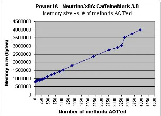
In Figure 7, we observe a complete view of the rise in memory size of the application as we

increase the number of methods that are AOT-compiled, including when we AOT-compile all the

methods of the application, in this case, 3955 methods. We can now appreciate the substantial

jump in memory size when the entire application is AOT-compiled. From an initial size of 794

This is why we mentioned that AOT compiling all the methods of the application is almost never

done practically.

Figure 7: Complete graph of Memory size vs. number of methods AOT’ed - CaffeineMark 3.0 on Neutrino/x86

Figure 8 illustrates a partial graph of the rise in memory size vs. the number of methods

compiled. For the sake of clarity, this graph illustrates data up to the point where we

AOT-compile 50 methods of the CaffeineMark application.

As we can observe, the memory size of the application increases as we increase the number

of methods that are AOT-compiled. This was expected, and serves to prove our earlier

assumption that the size of the Java application is smaller when the application is in bytecode

format, than when it is natively compiled. However, in this case, the top 2 to 3 percent of the hot

methods – 11 methods – are quite few in number as compared to the total number of methods in

the application. Therefore, there is only a marginal increase in the total memory size of the

application – of the order of ten to twenty kilobytes, when these methods are AOT-compiled.

This is a crucial point that should be kept in mind, and we will come back to this in the next few

paragraphs.

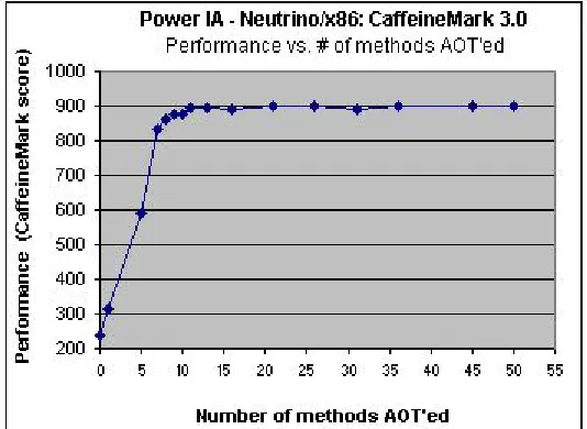
In Figure 9, we have an analysis of the change in performance as we increase the number of

methods that are AOT-compiled. Again, for the sake of clarity, we have displayed only a partial

graph, up to the point where we AOT-compile 50 methods.

Figure 9: Partial graph of Performance vs. number of methods AOT’ed - CaffeineMark 3.0 on Neutrino/x86

As can be clearly observed, there is a drastic rise in performance as we AOT-compile the top

methods. As we go on increasing the number of methods AOT-compiled, the performance keeps

on increasing until it reaches a saturation point, where the performance curve remains steady and

increases very marginally. In our case, for the figure above, this happens when we AOT-compile

11 methods onwards. We reiterate here that this saturation point is not the same for every

application, and may vary depending on the application type.

Figure 10 is a complete graph of performance change vs. number of methods AOT-compiled.

For all practical purposes, assuming that AOT compiling all the methods of the application

results in optimal, or close to optimal performance, we then obtain 983 as the optimal score of the

CaffeineMark benchmark on this platform.

Figure 10: Complete graph of Performance vs. number of methods AOT’ed - CaffeineMark 3.0 on Neutrino/x86

Hence, as we can observe in the figure above, we are able to achieve around 92% of the

optimal performance, just by AOT compiling the top 11 of the hot methods. We managed to

achieve 98.77% of the optimal performance by natively compiling around 160 methods (out of a

Finally, in Figure 11, we observe the crux of our results – change in performance as

compared to the corresponding increase in the memory size of the application. We reiterate here

the issues and difficulties that are faced in embedded environments. Embedded systems, unlike

their desktop counterparts, do not have the luxury of large memory space. Memory size is spoken

about in terms of kilobytes, rather than megabytes and gigabytes. Even a small increase in

memory could result in large monetary costs, considering that these embedded systems are

mass-produced.

Figure 11: AOT analysis of Performance vs. Memory size - CaffeineMark 3.0 on Neutrino/x86

From the figure above, we observe the steep rise in performance as we increase the number of

methods that are AOT-compiled. We were able to achieve 92% of the optimal performance at an

expense of about only 12 kilobytes, which worked out to an approximate increase of 2 percent in

the application’s memory size. This is a significant rise in performance, but the question that

remains to be asked is whether the embedded developer can afford that additional 12 KB? As we

said earlier, memory cost is usually crucial in the embedded world and even an increase as low as

It may so happen that the manufacturer of the embedded system may be entirely satisfied

with a performance score of 200. In that case, no further analysis would have to be conducted and

the application can be loaded onto the device without any changes or modifications. Similarly, for

real-time applications, it may be that all the deadlines are met and there is no need for any further

optimization.

However, if an increase in performance is imperative, then conducting an analysis like that

which we have outlined could be very useful. In Figure 12, we observe a zoomed-in view of the

change in performance as compared to the corresponding change in memory size. Embedded

system manufacturers may want a certain performance gain per kilobyte increase in memory size.

If they are able to achieve the performance gains within their tolerance for increase in memory

costs, then they might AOT-compile the additional methods. However, if the increased memory

costs are too high, they may prefer to sacrifice performance rather than incur these costs.

Figure 12: Partial graph of Performance vs. Memory size - CaffeineMark 3.0 on Neutrino/x86

Referring to Figure 12, we consider four data points as examples. The numbers adjacent to

the data points, i.e., 1, 5, 7, and 11, are the number of methods that are AOT-compiled at those

change in performance (CaffeineMark score). Calculating their respective values, we get x1 =

5792 bytes, y1 = 277 CaffeineMark points, x2 = 3232 bytes, and y2 = 61 CaffeineMark points.

For x1 and y1, the ratio of performance change to memory increase is 0.0478. For x2 and y2,

it is 0.0189. Clearly, for those developers that are interested in increasing performance, the

0.0478 ratio is well worth the investment. That is, a performance gain of 277 is obtained at a cost

of only 5792 bytes increase in memory. However, one might ask whether the 0.0189 ratio

(performance gain of 61) warrants the expenditure on the additional 3232 bytes. There is no

definite answer as to whether the 0.0189 ratio is worth the expense or not. At first glance, it

seems that we should AOT-compile 11 methods since that gives the maximum performance

benefit, and beyond that, the curve begins to level out. However, as we mentioned, the embedded

environment is different from that of the desktop, and what may seem to be the right decision

may not be the appropriate one. For example, it may so happen that the system manufacturer is

content with the performance benefit of AOT-compiling 7 methods, and may not want to bear the

additional memory cost of AOT compiling 11 methods. As we spoke about earlier, the developer

may have a certain tolerance limit for the rise in memory cost as the performance increases. The

memory cost for the performance gain in AOT compiling 7 methods may be within the

acceptable limit, but it may not be the case for AOT compiling 11 methods.

In this way, embedded developers can plot a graph of application performance versus

memory size increase. Using this, they can calculate the slope of the graph at various data points

– AOT compilation points, as we have shown in Figure 12. Finally, they can decide as to which

points are appropriate for their performance and memory size criteria. There is no clear-cut

answer as to how many methods should be precompiled for a particular application. It all depends

satisfactory. Others may prefer paying the extra cost of 3232 bytes and AOT compiling 11

methods in order to achieve even better performance. On the other hand, as we mentioned right at

the beginning, some developers may be satisfied with the initial performance of the application,

and may opt not to AOT-compile any method.

We reiterate here that the point in the curve, up to which the methods should be

AOT-compiled, will vary, depending on a few factors. One is the tolerance for the rise in memory size

that the developer is willing to incur. The developer may be faced with a fixed upper bound of

available memory space for the application. The application has to fit within this memory space,

no matter what the performance may be. The other tolerance limit is the one we spoke about

earlier; unless the ratio of performance change to memory increase is above a certain value, only

then may the cost be acceptable. Otherwise, performance may have to be sacrificed. Another

factor is the curve depicting the ratio of performance change to memory increase. In some cases,

as we will show for the SciMark application, the curve increases steeply very early on, and then

begins to flatten out. In some cases, the curve may increase less sharply and take a little longer

before it begins to saturate. Finally, there are cases, as shown for the CaffeineMark application in

Figure 12, which lie somewhere in between. It all depends on the characteristics of the

application, and the requirements of the developer/embedded system manufacturer.

Now referring back to Figure 11 on page 31, we observe that the performance curve begins to

level off after some time. After a certain point (11 methods in our case), there is only a marginal

increase in performance as more methods are AOT-compiled. In most cases, developers may not

proceed beyond this point, since there is only a slight benefit to be gained. However, it could so

happen that the embedded system has a certain amount of memory available, and the developers

may prefer to use all the available memory to extract every bit of performance. In that case,