Study of the Effect of Injection Pressure and Timing on the Combustion in an Optical Diesel Engine through Experiments and Simulations.

(1)

PADHIARY, ABHIJIT. Study of the Effect of Injection Pressure and Timing on the Combustion in an Optical Diesel Engine through Experiments and Simulations (Under the direction of Dr. Tiegang Fang).

(2)

(3)

Engine through Experiments and Simulations

By Abhijit Padhiary

A thesis submitted to the Graduate Faculty of North Carolina State University

in partial fulfillment of the requirements for the degree of

Master of Science

Mechanical Engineering

Raleigh, North Carolina 2018

APPROVED BY:

_______________________________ _______________________________ Dr. Stephen Terry Dr. Tarek Echekki

_______________________________ Dr. Tiegang Fang

(4)

DEDICATION

Dedicated to Krishna

(5)

BIOGRAPHY

(6)

ACKNOWLEDGMENTS

First, I would like to thank Dr. Fang for giving me the opportunity to work on combustion. The knowledge, skill and understanding that I have developed during this period of research is very important in my quest to understand combustion physics. He has been very patient, supportive and guided me during this project. Without his push and guidance, I would not have been able to develop the skills that helped me to carry out this work. I would like to thank Dr. Tarek Echekki and Dr. Stephen Terry for being understanding and accommodating during my thesis work. I specially thank Dr. Echekki for his lectures on fundamentals of combustion which have shaped my understanding.

I would like to take this opportunity to thank all my colleagues who have helped me with their inputs and support. Thanks a lot, Reuven, Libing, Kaushik, Fujun and Akash.

(7)

TABLE OF CONTENTS

LIST OF TABLES ... vi

LIST OF FIGURES ... vii

CHAPTER 1: INTRODUCTION ... 1

1.1 Background ... 1

1.2. Overview of combustion in CI engines ... 2

1.3. Literature review ... 4

1.4. Problem statement ... 5

CHAPTER 2: EXPERIMENTAL SETUP ... 7

2.1. Cummins SCE 903 ... 7

2.2. Optical access... 7

2.3. Drivetrain ... 8

2.4. Exhaust TDC signal and shaft encoder ... 8

2.5. Lubrication and coolant conditioning systems ... 8

2.6. Fuel injection System ... 9

2.7. Data acquisition system ... 10

2.8. High Speed Image acquisition system ... 11

CHAPTER 3: NUMERICAL MODEL ... 12

3.1. Overview of CONVERGE ... 12

3.2. Geometry... 12

3.3. Physical properties and Reaction Mechanism under ‘Materials’ section ... 16

3.4. Simulation parameters ... 17

(8)

3.6. Initial conditions and events ... 18

3.7. Physical Models ... 19

3.7.1. Spray Modelling... 19

3.7.2. Combustion Modelling ... 21

3.7.3. Turbulence Modeling ... 22

3.7.4. Grid Control ... 22

3.7.5. Output Processing ... 22

CHAPTER 4: RESULTS AND DISCUSSIONS ... 24

4.1. Design of Experiments ... 24

4.2. Data Analysis Methods ... 25

4.2.1. In-cylinder Volume ... 25

4.2.2. Pressure Referencing ... 25

4.2.3. Apparent Heat Release (AHR) and Mass Burned Fraction (MBF) ... 26

4.2.4. Burn Duration (CA 10, CA 50, CA 90) ... 26

4.2.5. Ignition Delay (ID) ... 27

4.2.6. NL Combustion images ... 27

4.2.7. Simulation Snapshots ... 28

4.2.8. Mass fractions vs Equivalence ratio at different CAD ... 29

4.3. Effects of Injection Pressure ... 29

4.4. Effects of Injection Timing ... 31

CHAPTER 5: CONCLUSION ... 85

(9)

LIST OF TABLES

Table 1. Specifications of the optical engine ... 7

Table 2. Time-step control parameter ... 17

Table 3. KH and RT parameters ... 21

(10)

LIST OF FIGURES

Figure 1 Phases of modern diesel engine ... 2

Figure 2 Front panel of Injection control system ... 10

Figure 3 Front panel of data acquisition program ... 11

Figure 4 ‘Make engine sector surface’ tool ... 14

Figure 5 Engine Sector Geometry ... 15

Figure 6 Rate Shape profile of the injector ... 21

Figure 7 Injection Pressure and Injection mass quantity used in CONVERGE simulations ... 25

Figure 8 A sample flame image (processed) through the optical window ... 28

Figure 9 A sample image (unprocessed) through the optical window ... 28

Figure 10 Pressure vs CAD curve for cases with SOI 10 CAD BTDC ... 32

Figure 11 Apparent Heat Release Rates vs CAD curve for cases with SOI 10 CAD BTDC ... 32

Figure 12 Apparent Heat Release vs CAD for cases with SOI 10 CAD BTDC ... 33

Figure 13 Mass Burnt Fraction vs CAD for cases with SOI 10 CAD BTDC ... 33

Figure 14 Ignition Delay vs CAD ... 34

Figure 15 Burn Duration vs CAD ... 34

Figure 16 Pressure vs CAD curve for cases with SOI 5 CAD BTDC ... 35

Figure 17 Apparent Heat Release Rates vs CAD curve for cases with SOI 10 CAD BTDC ... 35

Figure 18 Apparent Heat Release vs CAD for cases with SOI 10 CAD BTDC ... 36

(11)

Figure 20 Equivalence Ratio distribution snapshots in CAD for cases with

SOI 10CAD BTDC ... 37

Figure 21 Equivalence Ratio distribution snapshots in CAD for cases with SOI 5CAD BTDC ... 38

Figure 22 Mean Temperature with CAD for SOI 10CAD BTDC ... 39

Figure 23 Mean Temperature with CAD for SOI 5CAD BTDC ... 39

Figure 24 Natural Luminosity Images for Injection Pressure 800 bar, SOI 10 CAD BTDC ... 40

Figure 30 Combustion Development in case of 800 bar, SOI 10 CAD BTDC-1 ... 46

(12)

(13)

(14)

LIST OF ABBREVIATIONS TDC Top Dead Centre

BDC Bottom Dead Centre CI Compression Ignition BTDC Before Top Dead Centre ASOI After Start Of Injection SOI Start Of Injection ID Ignition Delay

(15)

CHAPTER 1: INTRODUCTION 1.1. Background

Internal combustion engines are the power house of modern society. Diesel engines have been the most preferred engine due to its higher efficiency and almost complete combustion of fuels leading to less emission of Carbon Dioxide (CO2). This is due to leaner combustion of fuels achieved through spray mixing of fuels. But in this process, they emit a large amount of other harmful pollutants like Nitrogen dioxide and particulate matter. There is a need to reduce the emissions while increasing the efficiency. Recent developments of high pressure injection systems (Common rail injection system) and turbocharging has made significant progress targeting this need. But there is still a long way to go to meet the upcoming emissions standards EPA TIER III, while still being very efficient. This motivates the researchers to gain the fundamental understanding of the spray combustion.

There is another method to reduce emissions, i.e. capturing the pollutants after they have been produced, classified as exhaust gas after treatment techniques. These include Diesel particulate filters and selective catalytic reduction techniques. But there is significant interest in reducing raw engine emissions while increasing the efficiency. Several methods like exhaust gas recirculation, high pressure injection system, multiple injections, injection rate shape alterations, combustion chamber geometry etc. are used by the research community to enhance the spray combustion in diesel engines.

(16)

effects of the fuel injection timing and pressure on the air fuel mixture preparation in a diesel engine through experiments and simulations.

1.2. Overview of combustion in C.I. Engines

The objective of this section is to introduce different processes in compressed ignition combustion engines and various parameters that can be used as indicators during the process. Different phases of CI combustion is shown in Figure 1.

Figure 1: Phases of modern diesel engine, adopted from [1]

(17)

evaporation and mixing. During the ignition delay, near to stoichiometric fuel air mixture is formed that leads to combustion initiation. Later the combustion can be classified into two types. Because of the ignition delay some of the fuel has already mixed with the air and thus it leads to premix combustion. As the premix combustion increases the temperature, there is a thin sheet of diffusion flame is formed where liquid fuel is vaporized and diffuses into the sheet to burn. This part of combustion is called diffusion flame. This is evident from the two peaks in the heat release curve, the first one is because of the premix combustion and the second peak is because of diffusion combustion.

One of the most important aspect of the combustion in diesel engines is the mixture preparation from the spray. When high pressure spray is injected into the chamber, the liquid spray breaks up because of the instabilities and shearing of the high pressure and temperature gasses. This breaks the liquid spray consisting of ligaments like structures into droplets which are then evaporated because of the surrounding temperature, thus leading to the formation of air and fuel mixture. When the air fuel mixture reaches a suitable ratio first reaction begins. The first reactions are slow, but the onset of spontaneous combustion provides further energy for accelerating this first set of reactions for remaining bulk of the fuel. This mixture formation shapes the combustion and subsequent emissions production.

(18)

temperature and volume fraction. Natural luminosity is an effective way to visualize combustion to interpret ignition and qualitative soot concentration.

1.3.Literature review

Effect of injection pressure on the diesel combustion was studied in an optical engine [2], which led to the conclusion that injection pressure increased the mixing and decreased the burn duration. This was even more evident with reducing impact of swirl on the chemiluminescence with the increasing injection pressure. The ignition was observed to occur near the wall.

Effect of injection pressure and timing on the spray mixing has been studied extensively among other parameters through computational models [3]. Lower injection pressure is found to have two peak distribution in terms of mixture fractions. Higher injection pressure gives a single peak of mass fraction in equivalence ratio space towards the spray tip showing higher air entrainment and mixing. It is shown that Injection timing advance can improve mixing but as we move towards TDC there is a rich distribution close to piston surface due to shorter clearance and more near the axis. Even though the model only studies non-combusting spray it gives a fair idea on the effects on injection pressure and timing on the mixture formation. In the numerical study [4] it has been found that increase in injection pressure leads to decrease in droplet size in the spray. The two peaks of droplet size distribution is also evident. Similar observation with respect to ignition delay and combustion duration is also found in [5].

(19)

presence of wall increases the mixing, which at higher injection pressures is magnified. This observation of fuel air mixing is higher aided by interaction with the wall is supported by [9]. Similar observation in parts is also found in [10], regarding the distribution of equivalence ratio. Similar conclusions of better mixing with increase in injection pressure is reached in [11],[12].

Ignition delay and combustion duration is generally found to decrease with increase in injection pressure [6],[13]. This is attributed to reduced droplet size and increase in air entrainment at higher injection pressure [4],[14],[15]. Moreover, injection timing has crucial role to play in the mixture formation as advanced injection timing provides more time for the fuel to mix and thus showing a higher premix combustion fraction. This gives rise to higher pressure rise rate and peak pressure[3],[13],[16]. But the temperature and density in engine conditions are not constant in engine conditions. Early injections face lower density, low temperature and longer penetration. Very early injection may lead to large increase in total ignition delay [17].

Ignition location in a spray and with the effect of flat plate is studied in [18]. This shows the offset of ignition in axial direction location because of the increased mixing near the wall. It is found to be at the tip of vapor spray closer to wall due to enhanced mixing [19],[20],[21].

Natural Luminosity can be an effective way to qualitatively compare the soot formation and flame structure[22],[23]. The studies in[24],[25],[26] show that increase in pressure effectively reduces soot NL. Similar to our experiments the work in [27] use NL images to compare different modes of combustion, showing the impact of injection pressure. The paper [23] provides guidelines for interpreting NL images.

1.4. Problem Statement

(20)

(21)

CHAPTER 2: EXPERIMENTAL SETUP 2.1. Cummins SCE 903

A Cummins VTE 903T engine, originally modifies by the US military for research purposes designated as SCE 903. The original V8 turbocharged engine was modified to a single cylinder, the details can be found in [28],[29]. All the essential components are modified for smooth running of the engine. Please note the compression ratio has changed as the piston was modified to flat top to provide optical access. For simplicity only, relevant details are provided in Table 1.

Table 1: Specifications of the optical engine

Engine Type Naturally Aspirated, Direct Injection

Bore 139 mm

Stroke 117 mm

Displacement 1.78 liters

Geometric Compression Ratio 12.9

Connecting Rod length 208.1 mm

Crank Arm Radius 58.5mm

2.2.Optical access

(22)

A classical Bowditch type of optical access is made whose details can be found in the thesis of previous students who worked on this setup [30],[31]. A schematic diagram shows the optical access in the engine and the optical insert.

2.3.Drive train

The optical engine is not able to power itself because of skip fire mode and low load-based injections. An external engine was used to drive the optical engine at constant speed of 600 RPM. Details about the engine can be found in [31].

2.4.Exhaust TDC signal and shaft encoder

A shaft encoder is coupled to the crank shaft, which is used to measure the transient crank angle degrees (CAD) for the data acquisition and control system. In simple lines the encoder generates a pulse every 0.5 CAD rotation, thus forming the basic grid for data acquisition and control.

The exhaust top dead center (TDC) signal is used as reference for the injection control and data acquisition. This is generated by a single tooth disc which rotates at half the speed of crank shaft and an optical switch circuit. The single tooth is synchronized to the TDC of optical engine, such that it generates a pulse at exhaust TDC. The pulse is generated by an optical switch whenever the tooth passes through it. More details can be found in [31].

2.5.Lubrication and coolant conditioning systems

(23)

2.6.Fuel injection System

The stock common rail system was modified to fit a commercial common rail and a 6 nozzle Bosch injector having 160 degrees spray angle. The system composed of a low-pressure pump followed by a high-pressure pump capable to inject the fuel above 1200 bars. Further details on the fuel injection system can be found in [31],[30].

The optical engine needs to run at low loads and skip fire mode (skip a few cycles between two batches of injection events) to prevent damage to the optical windows. For this purpose a control system was designed [31]. A feedback PID control loop consisting of rail pressure sensor controlled using NI myDAQ controller was used to achieve the target rail pressures. The controller reads the current rail pressure and calculates an error based on which a signal is given to the high-pressure pump to control the flow rate to achieve the target high-pressure.

A fuel injection control system was developed to account for skip fire mode injection [31]. Further improvement was also made to account for parameters

1. No. of skipped cycles 2. No. of injection cycles

3. Injection timing based on CAD.

(24)

Figure 2: Front panel of Injection control system

This control system however was not used wholly during the experimentation, but its features were included in the injection system used in experiments. More details on the exhaust TDC and CAD shaft encoder can be found in [30],[31].

2.7. Data acquisition system

(25)

further modified to enable to capture the time between two CAD, so as to correlate with the high-speed images, two counters from NI 6601 card. Figure 3 shows the front panel of the VI designed for this purpose.

Figure 3: Front panel of data acquisition program 2.8. High Speed Image acquisition system

(26)

CHAPTER 3: NUMERICAL MODEL 3.1.Overview of CONVERGE

Numerical modelling of the in-cylinder physics was performed using CONVERGE version 2.4. Diesel engine includes multiple processes like spray injection, droplet evaporation, fuel air mixing, combustion, emissions modelling, heat transfer, turbulence modelling etc. The method followed here is to solve the partial differential equation for pressure, density, temperature, species concentrations, velocities and turbulence parameters for gases and liquids at each grid for the whole domain. Converge uses finite volume method to solve for gas phase properties using Navier-Stokes equation. It uses the pressure implicit splitting of operator method (PISO) algorithm for the velocity pressure coupling. A variable time step is used subject to several accuracy and stabilizing limits. Sub grid scale modelling is used in spray modelling as it length and time scales are small. Further details on CONVERGE numerical methods can be found in the manual [32]. More details about the numerical model of the diesel engine is provided in the upcoming subsections. We have used CONVERGE studio to set up the case for simulation. All the case setup description will be based on the studio.

3.2.Geometry

(27)

(28)

(29)

Figure 5: Engine Sector Geometry

Swirl ratio used for the simulation is 0.8. Since the swirl ratio is not measured on this cylinder head, we have used the swirl ratio in [34], as the engine model used in their study is same as Cummins VT 903. The swirl profile used is standard profile recommended in [32]. The engine speed is 600 RPM.

(30)

include the crevice parameters, intake temperature, etc. More details on crevice parameters can be found in [32]. Application type is used as IC engines with CAD based simulation.

3.3.Physical properties and Reaction Mechanism under ‘Materials’ section

CONVERGE uses polynomial coefficients to obtain the gas properties which also can be obtained from an external therm.dat file (in NASA 7 or NASA 9 format) or a tabular format input file. A gas.dat file containing the viscosity and conductivity data is also required. A transport.dat file is also required. Since we will be using a surrogate fuel n-heptane to model Diesel 2 we will have to coerce the model to match the LHV of the original fuel. For this we use the LHV model available in CONVERGE. The LHV of n-heptane is coerced to 42.9 MJ/Kg.

The Liquid properties are set by the tabular format and Diesel 2 properties are used. A mech.dat file is used to provide the software with the reaction mechanism file that contains all the gas phase species and reaction data in it as we will be using SAGE detail chemistry model. Each reaction specified in mech.dat lists the pre-exponential factor𝐴𝐴𝑖𝑖, the temperature exponent𝑏𝑏𝑖𝑖, and the activation energy 𝐸𝐸𝑖𝑖 in the Arrhenius equation

𝑘𝑘𝑓𝑓𝑖𝑖 = 𝐴𝐴𝑖𝑖𝑇𝑇𝑏𝑏𝑖𝑖exp ( −𝐸𝐸𝐸𝐸_𝑅𝑅_𝑢𝑢_∗𝑇𝑇𝑖𝑖 ) (1)

(31)

3.4.Simulation parameters

Here we specify which file to get the geometry from, what properties to solve for and how the simulation will be controlled in terms of files and solver. All the files should be present in one directory for the solver to run. A transient solver with CAD temporal resolution is used. Simulation mode is ‘Full Hydrodynamic’ with compressible gas flow solver and incompressible liquid solver. We also specify to solve momentum and energy.

Simulation time is set from -180 CAD to 180 CAD. 0 CAD specifies the compression TDC of the engine. We used a variable time step algorithm where the minimum time step will be based on the models that are active at a particular point of time[32] and user defined CFL numbers. CFL numbers define the number of cells through which a related quantity can travel in one-time step. This gives freedom to accelerate the computation of certain models while going slowly for important models. Table 2 shows the time step parameters used for this model.

Table 2: Time-step control parameter

Initial Time step 5e-7

Minimum Time step 1e-8

Maximum Time step 2.5e-5

Maximum Convection CFL limit 1.0

Maximum Diffusion CFL limit 5.0

Maximum Mach CFL limit 50.0

(32)

Because of our computational limitations we have used recommended values for the solver parameters[32]. We have used strict conserve for all scalars and passives.

3.5.Boundary Conditions

As the name suggests in this setup we give the boundary conditions to the partial differential equations that will be solved. All the boundaries are given the temperature of coolant i.e. 170 F ~ 350 K.

I. Piston

Piston is given as ‘WALL’ boundary with translating motion specified as ‘piston motion’ in the case. The law of wall is used for the temperature boundary condition. It is generally used when turbulent boundary layer is not sufficient [32].

II. Front and Back Face

They are given ‘PERIODIC’ boundary as it allows us simulate only a sector of engine geometry[32].

III. Cylinder wall and cylinder head

They are given as stationary ‘WALL’ boundary and law of wall temperature boundary condition.

3.6. Initial conditions and events

In this section we can give initial conditions to the in-cylinder volume. Note, we are conducting numerical study in only the in-cylinder volume with the outside boundaries with wall boundary conditions. Since the effect of turbulence was not our key focus, we used typical values for the

simulation as prescribed by CONVERGE (Turbulent Kinetic Energy (TKE) = 62.0271𝑚𝑚2�_𝑠𝑠₂ and

Turbulent Dissipation = 17183.4𝑚𝑚2�_𝑠𝑠₃). Here we set the intake pressure at the end of intake stroke

(33)

temperature then used is 308 K (for 800 bar case). Further we can specify the intake air composition which also includes pollutant scalar compositions. We set the intake air composition as 79% Nitrogen and 21% Oxygen and specify the NOx scalar and soot scalar as 0.

3.7.Physical Models

In this section we specify which models to incorporate in our simulations. CONVERGE has a variety of models (which are based on various sub models). These include Spray, Combustion, emissions, turbulence, VOF, Fluid structure interaction etc. For our case we only used Spray, combustion, emissions and turbulence modelling. We will go through in details to explain our model. These details are very necessary for reproducing our results.

3.7.1. Spray Modelling

This section is explained in CONVERGE manual as ‘Discrete Phase Modelling’. They are in spray.in file. To simulate the spray in which liquid at high pressure is forced through nozzle leading to formation of droplets, CONVERGE uses parcels which are identical droplets (radius, composition, temperature etc.) to be placed at the injector nozzle location. The parcels statistically represent the spray by using different models to predict or given as input by the user. This is computationally very efficient. For simplicity we will only explain the models used for our case. Other models and their description can be found in [32].

(34)

mechanism file. To calculate the Spray penetration, we used 0.99 of the liquid mass for liquid spray penetration and 0.001 of vapor mass for fuel vapor penetration. The mass diffusivity constants are used that of diesel 2 with 1.0 scaling constants.

The Collison model used is NTC Collison model which is faster and more accurate than the only other Collison model available in CONVERGE (O’Rourke model)[37]. Because of computational limitations we have used less complex wall interaction (just rebound and slide) model. There was no available rate shape data on our injector, so we used existing rate shape profile which is almost a square rate shape, typical for the commercial injector. This profile is scaled based on the injection duration and the injection mass for the simulation. There may be variations in the simulation data with different injection rate shape profile. The rate shape profile is shown in the figure 6. A KH-RT breakup model is used in this case. Details about the model can be found in [32]. The parameters used are that of recommended for diesel injectors. They are also presented in Table 2. The injection timing and quantity was varied on the various cases which will be discussed the section cases setup. 1/6th_{of the total injection quantity was used since we are}

(35)

Figure 6: Rate Shape profile of the injector Table 3: KH and RT parameters

KH Shed Constant 1.0

KH Model Size constant 0.6

KH Model velocity constant 0.188 KH Model breakup time constant 7.0 RT Break up time constant 1.0

RT Model size constant 0.1

Coefficient of discharge 0.86

3.7.2. Combustion Modeling

(36)

In order to accelerate the computation we have used the option for analytical Jacobian and option to resolve rate constants only if temperature increases by 2K besides adaptive zoning (temperature bin size 5.0K, reaction ratio bin size 0.05) [32].

3.7.3. Turbulence modeling

For this case RANS RNG turbulence model is used with typical coefficients[32]. The focus of this work was not to account for the effects of various turbulence model so, we preferred to use less computationally expensive turbulence model. A heat transfer model based on [38] is used.

3.7.4. Grid Control

Base grid size used was 0.001 m. CONVERGE has the option to incorporate adaptive mesh refinement to resolve detail physics when there is a need to. A sub grid criterion level makes sure that the change in that property is resolved to maximum of this level in one cell. If required, this helps to add more cells till the change in one cell is below this level. Embedding level ensures how low the cell sizes can be. Velocity uses 2m/s sub grid criterion level with embedding of scale 2 (1/4 of cell size) throughout the simulation. Temperature uses sub grid criterion as 5 K and embedding scale of 2 but it is only activated during the combustion event. An embedding scale of 2 is used for the nozzle. This makes the smallest grid sizes to be 0.00025 m (0.25 mm) for the fixed embedding i.e. nozzle. A grid convergence study conducted in [39] finds this grid size to be grid convergent with SAGE model.. For the piston and cylinder head a scale of 1 is used.

3.7.5. Output processing

(37)

(38)

CHAPTER 4: RESULTS AND DISCUSSIONS 4.1. Design of Experiments

The experiments were designed to study the effect of injection pressure with three design points. The timing was studied with two design points for each injection pressure. The injection quantity was approximately constant for all the cases. Table 4 shows the experiments design very well.

Table 4: Design of Experiments

Case Injection Pressure Injection Timing Injection Quantity CAD duration 1 800 bars 10 CAD BTDC 46.29 mg (in experiment) 6.22

4 5 CAD BTDC 7.715*6 mg (in simulation)

2 1000 bars 10 CAD BTDC 46.26 mg (in experiment) 5.56

3 1200 bars 10 CAD BTDC 46.22 mg (in experiment) 5.08

(39)

Figure 7: Injection Pressure and Injection mass quantity used in CONVERGE simulations 4.2. Data Analysis Methods:

4.2.1. In-cylinder Volume

The volume of the cylinder(V) used for experimental data analysis was calculated using the equation given in [40]

𝑉𝑉

𝑉𝑉𝑐𝑐= 1 + 1

2× (𝑟𝑟𝑐𝑐−1) × [𝑅𝑅+ 1− 𝑐𝑐𝑐𝑐𝑠𝑠𝑐𝑐 −(𝑅𝑅2− 𝑠𝑠𝑠𝑠𝑠𝑠2𝑐𝑐)0.5] (2) Where, 𝑉𝑉_𝑐𝑐 = Clearance Volume (149.16 cc)

rc = compression ratio

R = Connecting rod length_{crank radius}

4.2.2. Pressure referencing

Pressure pegging with respect to intake manifold pressure is used to reference the relative pressure data recorded from the Kistler pressure sensor [31]. Average pressure during the intake is used to coerce the pressure measured at the end of intake stroke to generate absolute pressure

0 1 2 3 4 5 6 7 8 9 0 200 400 600 800 1000 1200 1400

0 1 2 3 4 5 6 7

In ject io n P res su re (b ar s) CAD

1000 bar, Injection Pressure

1200 bar, Mass Injected

1000 bar, Mass Injected

800 bar, Mass injected

(40)

data. Further to remove noise from the pressure data it is filtered with a seven-point moving average.

4.2.3. Apparent Heat Release (AHR) and Mass Burned Fraction (MBF)

During the combustion when fuel burns heat is released which is transferred to work into the piston. Of the total heat released a part of it is lost as heat to the walls. Remaining heat shows up in the work done by the pressure trace. AHR(𝑄𝑄_𝑛𝑛) can be calculated with realistic assumptions by[40]

𝑑𝑑𝑄𝑄𝑛𝑛 𝑑𝑑𝑑𝑑 = (

𝛾𝛾

𝛾𝛾−1×𝑝𝑝× 𝑑𝑑𝑉𝑉

𝑑𝑑𝑑𝑑) + ( 1

𝛾𝛾−1×𝑉𝑉× 𝑑𝑑𝑝𝑝

𝑑𝑑𝑑𝑑) (3)

Where, 𝛾𝛾 is the ratio of specific heat 𝐶𝐶𝑝𝑝

𝐶𝐶𝑣𝑣 (1.325 used in our calculations). 𝑑𝑑𝑄𝑄𝑛𝑛

𝑑𝑑𝑑𝑑 Can be integrated to find the total heat released (THR) during the cycle. Based on AHR a mass fraction burned fraction can be calculated. This can be analyzed to get a qualitative idea of progress of combustion in the cylinder.

𝑀𝑀𝑀𝑀𝑀𝑀(𝑋𝑋𝑏𝑏) = _{𝐴𝐴𝐴𝐴𝑅𝑅(𝑇𝑇𝑇𝑇𝑑𝑑𝐸𝐸𝑇𝑇)}𝐴𝐴𝐴𝐴𝑅𝑅 (𝐶𝐶𝐴𝐴𝐶𝐶) (4)

The heat transfer losses to the wall, crevice losses is assumed to have similar trends in all cases so that it will not have significant impact on the trends recognized in this thesis.

4.2.4. Burn Duration (CA 10, CA 50, CA 90)

(41)

4.2.5. Ignition Delay (ID)

Ignition delay in this work is measured using the Apparent Heat release curves (AHR) where it is quantified by the duration taken after the fuel injection to show the first sign of reaction[1],[40]. We use AHR curve to calculate the duration in CAD between the start of injection and when AHR curve becomes positive signifying that heat release has already started. Luminous delay is analogous to ID but it is defined as the duration between the start of injection and first visible light showing heat release reactions[19]. But because of inability of our setup to cover wide viewing area we were unable to calculate luminous delay effectively. We will be using the ID calculated from AHR for our analysis.

4.2.6. NL Combustion images

(42)

Figure 8: A sample flame image (processed) through the optical window

Figure 9: A sample image (unprocessed) through the optical window

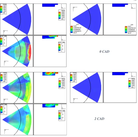
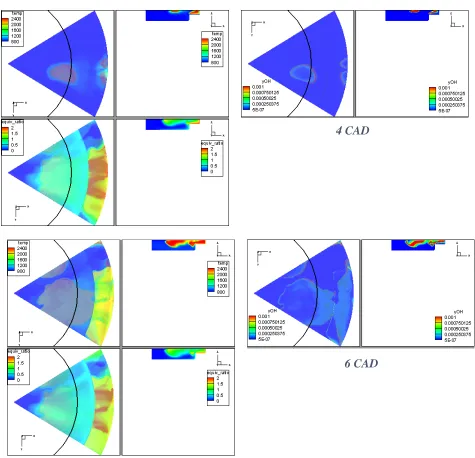
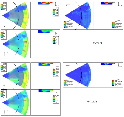
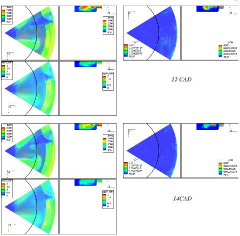
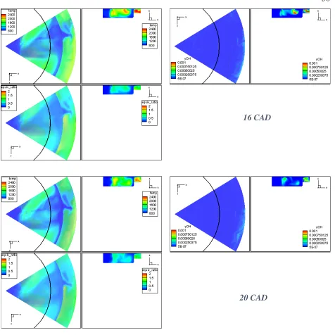
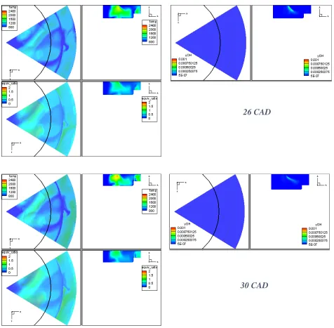
4.2.7. Simulation Snapshots

Simulation results are presented to show the evolution of combustion in all of the 6 cases. The pictures are made translucent to show the evolution along the same line of sight as

experiments. A side view of the middle plane is also provided to further strengthen such kind of representation. The semicircle indicates the extent of viewing area available through the

experiments. OH concentration and temperature are meant to show the flame and its evolution. Equivalence ratio is intended to indicate more details on the prevailing conditions of flame. They can also be used for qualitative comparison with the NL images obtained through experiments.

(43)

4.2.8.Mass fractions vs Equivalence ratio at different CAD

We have grouped cells with a close range of equivalence ratio and computed the mass fraction of the group. Such a mass fraction can give us an idea of the equivalence ratio

distribution at various CAD. Such a plot provides us with snapshots of premixing. 4.3. Effect of Injection Pressure:

To study the effect of injection pressure we kept the fuel mass, injection timing and all other parameters constant but varied the injection pressure. SOI for two set of cases are 350 CAD (10 CAD BTDC) and 355 CAD (5 CAD BTDC). Figure 10 shows the Pressure curves for 350 CAD injection (10 CAD BTDC). Due to lack of ambient conditioning system we were not able to keep the intake temperature at a constant value but since the experiments are conducted one after another, the intake temperatures are very close to each other (308 for 800 bar cases to 315 K for 1200 bar). We expect this will not impact the trends we are trying to observe.

(44)

(45)

structures include chemiluminescence from OH and soot radiation, which depends on soot temperature).

4.4. Effect of injection timing:

Simulations and experiments are carried out to understand the influence of injection timing for two different cases 10 CAD BTDC and 5 CAD BTDC. Earlier injection timing gives enough time to the fuel to mix thus leading to larger premix fractions and peak pressures. This is because of faster heat release rates. At 5 CAD BTDC SOI cases leaning of the mixture is not seen as in 10 CAD BTDC SOI injection cases. Because of absence of leaning due to large premixing of charge there is smooth combustion (evident in mass burnt fraction). This may result in low heat transfer losses thus leading to more apparent heat release. Most of combustion in 5 CAD BTDC SOI occurs outside our view in the squish region. The cases with SOI 5 CAD BTDC have slightly larger burn duration with lower peak pressures and heat release rates.

(46)

Figure 10: Apparent Heat Release Rates vs CAD curve for cases with SOI 10 CAD BTDC

Figure 11: Apparent Heat Release Rates vs CAD curve for cases with SOI 10 CAD BTDC

0 1 2 3 4 5 6

300 310 320 330 340 350 360 370 380 390 400 410 420

P(

θ

)

CAD 800 bar-10, Experimental

800 bar -10, Simulated 1000 bar -10, Experimental 1000 bar -10, Simulated 1200 bar -10, Experimental 1200 bar -10, Simulated Motoring, Simulated Motoring, Experimental -50 50 150 250 350 450 550

350 360 370 380 390 400 410 420

AH

RR (J

)

CAD

(47)

Figure 12: Apparent Heat Release vs CAD for cases with SOI 10 CAD BTDC

Figure 13: Mass Burnt Fraction vs CAD for cases with SOI 10 CAD BTDC

-150 50 250 450 650 850 1050 1250 1450

340 350 360 370 380 390 400 410 420

AH

R (J

)

CAD

800 bar-10, Experimental 800 bar -10, Simulated 1000 bar -10, Experimental 1000 bar -10, Simulated 1200 bar -10, Experimental 1200 bar -10, Simulated

0 0.1 0.2 0.3 0.4 0.5 0.6 0.7 0.8 0.9 1

340 350 360 370 380 390 400 410 420

Xb(M as s bur nt Fr act io n) CAD

(48)

Figure 14: Ignition Delay vs CAD

Figure 15: Burn Duration vs CAD

0 2 4 6 8 10

700 800 900 1000 1100 1200 1300

Ig ni tio n De la y ( CA D)

Injection Pressure (bars) Experimental, SOI 10 BTDC

Simulation, SOI 10 BTDC

Experimental, SOI 5BTDC

Simulation, SOI 5BTDC

8 10 12 14 16 18 20 22 24 26 28 30 32 34 36 38 40

800 900 1000 1100 1200

Dur

ati

on (

CA

D)

Injection Pressure (bars)

(49)

Figure 16: Pressure vs CAD curve for cases with SOI 5 CAD BTDC

Figure 17: Apparent heat release rates vs CAD curve for cases with SOI 5 CAD BTDC

0 1 2 3 4 5 6

300 310 320 330 340 350 360 370 380 390 400 410 420

P( θ ) CAD Motoring, Simulated Motoring, Experimental 800 bar-5, Simulated 800 bar-5, Experimental 1200 bar -5, Experimental 1000 -5, Simulated 1000 bar -5, Experimental 1200 -5, Simulated

-50 0 50 100 150 200 250 300 350 400 450

350 370 390 410

AH

RR (J

)

CAD

800 bar-5, Experimental

800 bar -5, Simulated

1000 bar -5, Experimental

1000 bar -5, Simulated

1200 bar -5, Experimental

(50)

Figure 18: Apparent heat release vs CAD curve for cases with SOI 5 CAD BTDC

Figure 19: Mass Burn Fraction vs CAD curve for cases with SOI 5 CAD BTDC

-150 50 250 450 650 850 1050 1250 1450

340 350 360 370 380 390 400 410 420

AH

R (J

)

CAD

800 bar-5, Experimental 800 bar -5, Simulated 1000 bar -5, Experimental 1000 bar -5, Simulated 1200 bar -5, Experimental 1200 bar -5, Simulated

0 0.1 0.2 0.3 0.4 0.5 0.6 0.7 0.8 0.9 1

340 350 360 370 380 390 400 410 420

Xb(M as s bur nt Fr act io n) CAD

800 bar-5, Experimental 800 bar -5, Simulated 1000 bar -5, Experimental

1000 bar -5, Simulated 1200 bar -5, Experimental

(51)

Figure 20: Equivalence Ratio distribution snapshots in CAD for cases with SOI 10CAD BTDC 0.00E+00 5.00E-02 1.00E-01 1.50E-01 2.00E-01 2.50E-01

0 0.2 0.4 0.6 0.8 1 1.2 1.4 1.6 1.8 2

M as s F rac tion Equivalence ratio

5 CAD ASOI 10CAD ASOI 15 CAD ASOI 20 CAD ASOI 25 CAD ASOI 30 CAD ASOI 35 CAD ASOI 40 CAD ASOI 45 CAD ASOI

Injection Pressure: 1000 Bar SOI 10CAD BTDC

0.00E+00 5.00E-02 1.00E-01 1.50E-01 2.00E-01 2.50E-01

0 0.2 0.4 0.6 0.8 1 1.2 1.4 1.6 1.8 2

5 CAD ASOI 10CAD ASOI 15 CAD ASOI 20 CAD ASOI 25 CAD ASOI 30 CAD ASOI 35 CAD ASOI 40 CAD ASOI 45 CAD ASOI

0.00E+00 5.00E-02 1.00E-01 1.50E-01 2.00E-01 2.50E-01

0 0.2 0.4 0.6 0.8 1 1.2 1.4 1.6 1.8 2

5 CAD ASOI 10 CAD ASOI 15 CAD ASOI 20 CAD ASOI 25 CAD ASOI 30 CAD ASOI 35 CAD ASOI 40 CAD ASOI 45 CAD ASOI

(52)

Figure 21: Equivalence Ratio distribution snapshots in CAD for cases with SOI 5CAD BTDC 0.00E+00 5.00E-02 1.00E-01 1.50E-01 2.00E-01 2.50E-01

0 0.2 0.4 0.6 0.8 1 1.2 1.4 1.6 1.8 2

M as s Fr ac tio n Equivalence ratio

0.00E+00 5.00E-02 1.00E-01 1.50E-01 2.00E-01 2.50E-01

0 0.2 0.4 0.6 0.8 1 1.2 1.4 1.6 1.8 2

0.00E+00 5.00E-02 1.00E-01 1.50E-01 2.00E-01 2.50E-01

0 0.2 0.4 0.6 0.8 1 1.2 1.4

(53)

Figure 22: Mean Temperature with CAD for SOI 10CAD BTDC

Figure 23: Mean Temperature with CAD for cases with SOI 5 CAD BTDC

600 700 800 900 1000 1100 1200 1300 1400 1500 1600

360 365 370 375 380 385 390 395 400

Me an Te m pe ra tur e ( K) CAD

Injection Pressure 800 bar, -10 SOI

600 700 800 900 1000 1100 1200 1300 1400 1500 1600

360 365 370 375 380 385 390 395 400

Me an Te m pe ra tur e ( K) CAD

(54)

Figure 24: Natural Luminosity Images for Injection Pressure 800 bar, SOI 10 CAD BTDC

16 18 20

24 30 34

44 54 64

10 12 14

(55)

Figure 25: Natural Luminosity Images for Injection Pressure 1000 bar, SOI 10 CAD BTDC 9

7 5

11 13 15

17 19 21

25 31 35

(56)

14 12

10 8

4

18 20 22

26 30 36

(57)

14 15 17

19 21 23

25 27 29

31 33 39

(58)

23

13 15 17

19 21

25 27 29

31 33 35

(59)

11 13 15

17 19 21

23 25

29 31 33

(60)

Figure 30: Combustion Development in case of 800 bar, SOI 10 CAD BTDC-1

0 CAD

(61)

4 CAD

(62)

(63)

12 CAD

(64)

16 CAD

(65)

26 CAD

(66)

40 CAD

(67)

0 CAD

(68)

4 CAD

(69)

Figure 39: Combustion Development in case of 1000 bar, SOI 10 CAD BTDC-3

8 CAD

(70)

12 CAD

(71)

16 CAD

(72)

26 CAD

(73)

40 CAD

(74)

0 CAD

(75)

4 CAD

(76)

8 CAD

(77)

12 CAD

(78)

16 CAD

(79)

(80)

40 CAD

(81)

4 CAD

(82)

8 CAD

(83)

12 CAD

(84)

16 CAD

(85)

20 CAD

(86)

36 CAD

(87)

4 CAD

(88)

8 CAD

(89)

12 CAD

(90)

16 CAD

(91)

20 CAD

(92)

36 CAD

(93)

4 CAD

(94)

8 CAD

(95)

12 CAD

(96)

16 CAD

(97)

20 CAD

(98)

36 CAD

(99)

CHAPTER 5: CONCLUSION

Experiments and simulations were conducted with diesel for 3 cases of different pressure and 2 cases of injection timing with the aim to understand the evolution of combustion via experimental and numerical approaches. Numerical experiments were seen to closely follow experimental results showing important trends of combustion in diesel fuel. The conclusions are as follows.

1. Ignition is found to occur in the vicinity of wall where the spray interacts with the wall with enhanced mixing. Our experimental setup is not able to capture the ignition and combustion at early stages due to narrow view. But our simulation results show the point of combustion and its evolution.

2. Increasing the injection pressure increases the spray break up and mixing. Thus resulting in a faster and more premix type of combustion. This led to larger heat release rates and peak pressures. Equivalence ratio profiles obtained show enhanced mixing in a reacting spray with increase in injection pressures.

(100)

REFERENCES

[1] J. E. Dec, “A Conceptual Model of DI Diesel Combustion Based on Laser-Sheet Imaging*,” SAE Tech. Pap., Feb. 1997.

[2] M. K. Le and S. Kook, “Injection Pressure Effects on the Flame Development in a Light-Duty Optical Diesel Engine,” SAE Int. J. Engines, vol. 8, no. 2, pp. 2015-01–0791, 2015. [3] J. Abraham, “Computational study of charge stratification in early-injection SCCI engines

under light-load conditions,” Int. J. Automot. Technol., vol. 12, no. 5, pp. 721–732, 2011. [4] A. R. Andsaler et al., “The effect of nozzle diameter, injection pressure and ambient

temperature on spray characteristics in diesel engine,” J. Phys. Conf. Ser., vol. 822, no. 1, p. 12039, Apr. 2017.

[5] J. Jeon, J. T. Lee, S. Il Kwon, and S. Park, “Combustion performance, flame, and soot characteristics of gasoline–diesel pre-blended fuel in an optical compression-ignition engine,” Energy Convers. Manag., vol. 116, pp. 174–183, May 2016.

[6] T. Kakegawa, T. Suzuki, K. Tsujimura, and M. Shimoda, “A Study on Combustion of High Pressure Fuel Injection for Direct Injection Diesel Engine,” SAE Int., Feb. 1988.

[7] G. Bruneaux, “Mixing Process in High Pressure Diesel Jets by Normalized Laser Induced Exciplex Fluorescence Part II: Wall Impinging Versus Free Jet,” SAE Int., May 2005. [8] G. Bruneaux, “Mixing Process in High Pressure Diesel Jets by Normalized Laser Induced

Exciplex Fluorescence Part I: Free Jet,” SAE Int., May 2005.

[9] L. M. Pickett and J. J. López, “Jet-Wall Interaction Effects on Diesel Combustion and Soot Formation,” SAE Int., Apr. 2005.

(101)

Local Fuel Mixture Fraction,” SAE Int. J. Engines, vol. 4, no. 1, pp. 2011-01–0686, Apr. 2011.

[11] T. Fang, C.-F. Lee, R. Coverdill, and R. White, “Effects of Injection Pressure on Low-sooting Combustion in an Optical HSDI Diesel Engine Using a Narrow Angle Injector,” SAE Int., Apr. 2010.

[12] X. Wang, Z. Huang, O. A. Kuti, W. Zhang, and K. Nishida, “Experimental and analytical study on biodiesel and diesel spray characteristics under ultra-high injection pressure,” Int. J. Heat Fluid Flow, vol. 31, no. 4, pp. 659–666, Aug. 2010.

[13] A. K. Agarwal, D. K. Srivastava, A. Dhar, R. K. Maurya, P. C. Shukla, and A. P. Singh, “Effect of fuel injection timing and pressure on combustion, emissions and performance characteristics of a single cylinder diesel engine,” Fuel, vol. 111, pp. 374–383, 2013. [14] N. Kawaharada, D. Sakaguchi, H. Ueki, and M. Ishida, “Effect of Injection Pressure on

Droplet Behavior Inside Diesel Fuel Sprays,” SAE Int., Sep. 2015.

[15] M. T. Shervani-Tabar, M. Sheykhvazayefi, and M. Ghorbani, “Numerical study on the effect of the injection pressure on spray penetration length,” Appl. Math. Model., vol. 37, no. 14–15, pp. 7778–7788, Aug. 2013.

[16] H. J. Kim, S. H. Park, and C. S. Lee, “Impact of fuel spray angles and injection timing on the combustion and emission characteristics of a high-speed diesel engine,” Energy, vol. 107, pp. 572–579, Jul. 2016.

[17] X. Fu and S. K. Aggarwal, “Two-stage ignition and NTC phenomenon in diesel engines,” Fuel, vol. 144, pp. 188–196, Mar. 2015.

(102)

[19] P. M. Lillo, L. M. Pickett, H. Persson, O. Andersson, and S. Kook, “Diesel Spray Ignition Detection and Spatial/Temporal Correction,” SAE Int. J. Engines, vol. 5, no. 3, pp. 2012-01–1239, Apr. 2012.

[20] C. Chartier, U. Aronsson, Ö. Andersson, and R. Egnell, “Effect of Injection Strategy on Cold Start Performance in an Optical Light-Duty DI Diesel Engine,” SAE Int. J. Engines, vol. 2, no. 2, pp. 431–442, Sep. 2009.

[21] T. Huelser et al., “Mixture-Formation Analysis by PLIF in an HSDI Diesel Engine Using C 8 -Oxygenates as the Fuel,” SAE Int. J. Fuels Lubr., vol. 8, no. 2, pp. 2015-01–0960, Apr.

2015.

[22] J. E. Dec and C. Espey, “Ignition and Early Soot Formation in a DI Diesel Engine Using Multiple 2-D Imaging Diagnostics,” SAE Int., Feb. 1995.

[23] C. J. Mueller and G. C. Martin, “Effects of Oxygenated Compounds on Combustion and Soot Evolution in a DI Diesel Engine:Broadband Natural Luminosity Imaging,” SAE Int., no. 724, May 2002.

[24] T. G. Fang, R. E. Coverdill, C. F. F. Lee, and R. A. White, “Low-sooting combustion in a small-bore high-speed direct-injection diesel engine using narrow-angle injectors,” Proc. Inst. Mech. Eng. Part D J. Automob. Eng., vol. 222, no. 10, pp. 1927–1937, 2008.

[25] J. Zhu, O. A. Kuti, and K. Nishida, “Effects of Injection Pressure and Ambient Gas Density on Fuel - Ambient Gas Mixing and Combustion Characteristics of D.I. Diesel Spray,” SAE Int., Aug. 2011.

(103)

conventional and low temperature diesel combustion,” Appl. Energy, vol. 119, pp. 454–466, Apr. 2014.

[28] D. M. Y. (SwRI) Lacey, P.I., E.A. Frame, “SINGLE-CYLINDER ENGINE EVALUATIONS OF HIGH-TEMPERATURE LUBRICANTS FOR U . S . ARMY GROUND VEHICLES,” 1992.

[29] C. R. Mure and K. T. Rhee, “Instantaneous Heat Transfer over the Piston of a Motored Direct injection Type Diesel Engine,” in SAE International, 1989, vol. 890469.

[30] A. Mccullough, “Construction and Design Verification of a Heavy-Duty Optical Engine Test Bed,” NC State University, 2015.

[31] R. J. Gomes, “Testing of Diesel, BTL and Jet-A Fuel using a 1.8L Heavy Duty Optical Engine Test-Bed with High Speed Visualization Techniques,” North Carolina State University, 2017.

[32] E. Richards, K. J., Senecal, P.K., and Pomraning, “Converge 2.4 Manual,” Madison, WI, 2018.

[33] P. K. Senecal, E. Pomraning, K. J. Richards, and S. Som, “Grid-Convergent Spray Models for Internal Combustion Engine CFD Simulations,” in ASME 2012 Internal Combustion Engine Division Fall Technical Conference, 2012, p. 697.

[34] P. Schihl, J. Tasdemir, and W. Bryzik, “Determination of Laminar Flame Speed of Diesel Fuel for Use in a Turbulent Flame Spread Premixed Combustion Model,” Warren, MI, 2004.

(104)

[36] Fabian Mauß, “Entwicklung eines kinetischen Modells der Rußbildung mit schneller Polymerisation,” RWTH Aachen, 1996.

[37] D. P. Schmidt and C. J. Rutland, “A New Droplet Collision Algorithm,” J. Comput. Phys., vol. 164, no. 1, pp. 62–80, Oct. 2000.

[38] A. A. Amsden, P. J. O’Rourke, and T. D. Butler, “KIVA-II: A Computer Program for Chemically Reactive Flows with Sprays,” Los Alamos Natl. Lab., p. LA-11560-MS, 1989. [39] S. Som et al., “A Numerical Investigation on Scalability and Grid Convergence of Internal

Combustion Engine Simulations,” in 2013 SAE World Congress & Exhibition, 2013. [40] J. B. Heywood, Internal Combustion Engine Fundamentals. New York: McGraw-Hill,