Abstract
NIEUWENHUIS, BRIAN PAUL. A study of Severe Thunderstorm Interaction with Thermal Boundaries: Collision Angle and Stability. (Under the direction of Al Riordan.)
It has been observed many times that thunderstorm cells which interact with
thermal boundaries frequently become severe or tornadic. It has also been noted in some
past studies that while some storms cross a boundary and dissipate, other storms turn at
the boundary and produce severe weather as they travel along the baroclinic zone. A
number of severe thunderstorm cases have been observed and analyzed to determine what
makes some storms turn and others not. The angle that the storm approached the
boundary was investigated, as well as various stability factors, the strength of the
boundary, and the speed and intensity of the storms. It was found that there is a
relationship between the angle of approach and the fate of the cell, and that the
relationship can change depending on certain environmental factors. With further
research, this knowledge may become useful for future operational severe weather
A STUDY OF SEVERE THUNDERSTORM INTERACTION WITH THERMAL BOUNDARIES: COLLISION ANGLE AND STABILITY
by
BRIAN PAUL NIEUWENHUIS
A thesis submitted to the graduate faculty of North Carolina State University
in partial fulfillment of the requirements for the Degree of
Master of Science
MARINE EARTH AND ATMOSPHERIC SCIENCES
Raleigh
2006
APPROVED BY:
________________________ ________________________
Biography
Brian was born on March 16th, 1981, to a loving family in Kernersville, North Carolina. Throughout his childhood he experienced different weather phenomenon
which in turn sparked his interest in meteorology. In 1999, he attended the University of
North Carolina at Asheville and received a Bachelors Degree in Atmospheric Sciences.
To further pursue his interest in meteorology he attended graduate school at North
Carolina State University in 2003. Throughout his years of college education, he met his
wife Melissa at UNC-Asheville and was blessed with a son in 2005. Upon receiving his
Acknowledgments
Thanks to Kermit Keeter and Jonathan Blaes of the NWS LFO Raleigh, NC for
help with data and graphics. Helpful comments and suggestions and data access were
provided by Drs. Gary Lackmann, Matt Parker, and Sethu Raman from the MEAS Dept
at NCSU. Thanks also to Ranae Mistarz for providing thoughtful review. Special thanks
Table of Contents
page
LIST OF TABLES . . . vi
LIST OF FIGURES . . . . vii
INTRODUCTION . . . 1
LITERATURE REVIEW . . . 2
METHOD . . . 7
Methodology applied . . . 12
RESULTS . . . 14
Case studies . . . 14
June 4. 2004 . . . 15
March 22, 2005 . . . 17
Overall results . . . 19
CONCLUSIONS . . . 22
List of Tables
page
Table 1. Spreadsheet showing all cases and relevant
List of Figures
page
Figure 1. Surface map for 15Z March 27, 1994. . . . . 28
Figure 2. Tornado track map from Palm Sunday Outbreak. . . 28
Figure 3. Schematic of typical wind profile through
a surface frontal system. . . . . 29
Figure 4. Schematic of boundary intensification processes. . 30
Figure 5. Initialization of the COMMAS model to study boundary effects on cell development,
intensification, and track. . . . . 31
Figure 6. Typical identification of turning storms and
non-turning storms. . . . . . . 32
Figure 7. A schematic representing the process of
measuring the angle of intersection between the
boundary and the cell. . . . 33
Figure 8. Schematic showing the determination of significant error in intersection angle measurement. . . . 33
Figure 9. Surface conditions at 15Z and 18Z on J
June 4, 2004. . . . . 34
Figure 10. Maps used during methodology for boundary
placement and cell #3 tracking on June 4, 2004. . 35
Figure 11. Radar images showing how storm tracking was done for cell #3 on June 4, 2004. . . . . . 36
Figure 12. Map used to make final intersection angle
measurement for cell #3 on June 4, 2004. . . . 37
Figure 13. Error schematic for cell track for case #3
on June 4, 2004. . . . . 37
Figure 14. Error schematic for boundary placement at 15Z
on June 4, 2004. . . . . 38
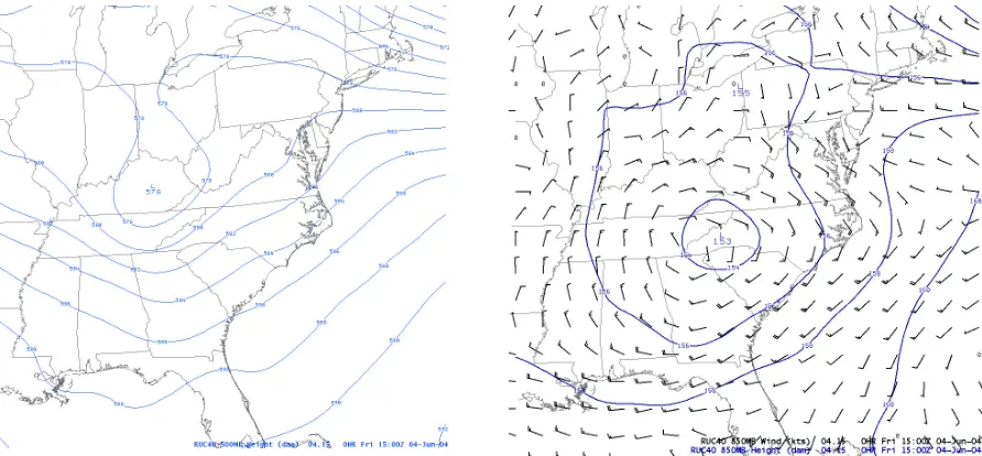
Figure 15. 500mb (left) and 850mb (right) contours for
Figure 16. CAPE across North Carolina at 15Z on
June 4, 2004. . . . . . . 39
Figure 17. CIN across North Carolina at 15Z on
June 4, 2004. . . . . 39
Figure 18. Composite radar imagery for 15Z on
June 4, 2004. . . . . 40
Figure 19. Composite radar imagery for 16Z, 18Z,
and 21Z on June 4, 2004. . . . . . 40
Figure 20. Radar and infrared satellite imagery from
June 4, 2004, showing cell intensification. . . 41
Figure 21. Storm-relative velocity imagery at 16Z and
19Z from June 4, 2004. . . . 41
Figure 22. A comparison of storm reports with surface
boundaries on June 4, 2004. . . . . . 42
Figure 23. Surface map for March 22, 2005 at 19Z. . . . 43
Figure 24. 850mb isoheights and 250mb wind vectors for
March 23, 2005 at 00Z. . . . 43
Figure 25. Sounding from Tallahassee at 00Z on
March 23, 2005. . . . . 44
Figure 26. Radar image from 15Z on March 22, 2005. . . . 44
Figure 27. Schematic showing the updraft cut-off process. . 45
Figure 28. Map of some tornado tracks from March 22, 2005. . 45
Figure 29. Comparison of CAPE and intersection angle. . . 47
Figure 30. Comparison between CIN and intersection angle. . 48
Figure 31. Comparison of time-of-occurrence to
intersection angle. . . . . 49
Figure 32. Comparison of storm cell speed and
intersection angle. . . . . 49
Figure 33. Comparison of boundary strength with
Introduction
On the morning of March 27, 1994, Palm Sunday, the synoptic situation in the
Southeast United States showed few of the “classic” signs of strong thunderstorm
development (NOAA, 1994). Nevertheless, within hours, severe weather had begun and
before the end of the day, nearly 30 tornadoes had touched down across Alabama,
Georgia, and the Carolinas, two of them reaching F-4 strength. In strong southwesterly
flow, supercells and other storms approached a stationary front in place in northern
Georgia and Alabama. The environment near the event had no organized areas of positive
vorticity advection (PVA), and exhibited no evidence of synoptic-scale jet or
quasigeostrophic forcing (Koch et al. 1998). However, the boundary provided enhanced
lifting, and as a result, became the focus of large hail and tornadoes. In total, 42 deaths,
320 injuries, and over $100 million in damages were the result of the day’s activity.
The main reason for the active convection of that day evidently lay in the
enhanced lifting associated with the frontal boundary. With Convective Available
Potential Energy (CAPE) values from 1000-2000 J/Kg, and nearly 0 J/Kg Convective
Inhibition (CIN) values, the environment was more than conducive to active convection.
Those storms that produced the longest lived and most intense tornadoes had intersected
the front and changed direction to follow along its boundary. Others had crossed the
boundary and dissipated on the cool side. It was observed that as long as the cells were
in the vicinity of the front, they experienced rapid growth and intensification (Langmaid
and Riordan 1998). Figures 1 and 2 show the synoptic surface features and the tracks of
It was noted by the authors that the cells that changed course to follow the
boundary approached the front at a smaller angle than those storms that fully crossed the
boundary, and those that did alter course may have existed in more unstable
environments than those that crossed into the cold air and dissipated. It is the purpose of
this research to investigate if there is a critical angle of intersection which determines if a
given storm cell will intensify and move along a boundary, or cross and dissipate. The
research will also seek to determine if the critical angle is related to the stability
conditions of the storm environment. The collision speed between the cell and the
boundary, the boundary intensity, and initial cell intensity will also be studied for similar
relationships.
It is hypothesized that a critical angle does exist and that the angle increases as
the static stability decreases. It is also believed that wind shear along the boundary has
an impact on storm behavior.
Literature Review
The effect of baroclinic boundaries on the development and intensification of
convective storms has been a major topic of research for many years (Magor 1959; Miller
1972; etc.). Most of this research has focused on the significance of the boundaries, and
how they influence the development and track of thunderstorm cells.
Maddox et al. (1980) recognized that boundary zones have long been recognized
as important regions for storm development, and therefore conducted a study of
is the predominant catalyst for severe weather. They found that a storm cell that has a
track normal to a boundary tends to produce a short-lived, but intense storm. However, a
storm that has a track parallel to a boundary tends to produce a longer-lived intense
storm. As long as the cell remains within the frontal zone, it remains more intense than if
there were no boundary present.
Maddox explains the intensification with an analysis of wind shear. As winds on
the cold side of the boundary and in the warm sector veer slowly with height, the winds
on the cool side veer much faster, as shown in Figure 3. Considering only the mean
sub-cloud layer winds, this veering difference creates surface moisture convergence and
vorticity maxima across a narrow area along the baroclinic zone. This area of maxima
then acts to intensify any convection that it encounters.
During the Verification of the Origins of Tornadoes Experiment (VORTEX-95),
Markowski et al. (1998) found that 70% of tornadoes studied were associated with a
boundary interaction: either within 10 km on the warm side or 30 km on the cool side. In
this study the intensification is explained with horizontal, or solenoidal, vorticity
generated by the boundary. Boundaries had previously been theoretically shown to
produce areas of strong (~10^-2 /s) horizontal vorticity (Klemp and Rotunno 1983;
Rotunno et. al. 1988; Rasmussen and Rutledge 1993a, 1993b). It has also been shown
that if a strong updraft enters this area, the vorticity can be tilted vertically and stretched,
creating a stronger updraft region, thereby strengthening the cell (Weismann and Klemp
1982; Klemp and Rotunno 1983). Markowski noticed during VORTEX-95 that storms
that remained close to the boundary lasted much longer than those that crossed
better chance to take advantage of the inherent instability and vorticity in order to
maintain and intensify than those cells that cross the boundary completely. See Figure 4
for a visual representation of this process.
The vorticity stretching and tilting has also been verified in studies by Wakimoto
et al. (1998), and Rasmussen et al. (2000). Rasmussen in particular found that storm cells
that crossed a thermal boundary experienced a significant increase in storm rotation and
an increase of inflow rates averaging from 30 m/s to 42 m/s. Brady and Szoke (1989)
used a high-resolution radar to research a storm/boundary interaction and noted that the
boundary’s pre-existing horizontal vorticity was stretched and tilted vertically, resulting
in a tornado developing within the intensifying cell.
Including tornadoes, a majority of severe weather may occur near or on surface
boundaries. For example, nearly all severe thunderstorm flooding and flash flooding
events between 1992 and 1998 in the continental United States occurred on or near a
surface boundary (Rogash and Racy 2002). The boundaries that produce severe weather
by interaction with storm cells are most often mesoscale in nature, i.e.: a gust front from
another cell. However, others can be synoptic type fronts and the two scales can have
much of the same effect on various cells (Marshall et al. 2002). In fact, nearly 21% of all
intense tornadoes in a study by Johns et al. (2000) were along or just to the cool side of
thermal boundaries, with occluded, stationary, and warm fronts being the most likely to
produce severe to tornadic thunderstorms. Broyles et al. (2002) found that of all violent
tornado tracks studied, 43% were associated with a frontal boundary, and 16% were
Typically, in the absence of a boundary, a steady-state thunderstorm’s motion
follows that of the mean wind in the cloud layer. Should the storm become stronger, and
begin to develop new convection to the right of the motion, then the storm tends to move
just to the right of the mean wind, i.e. a right-moving supercell. However, in the
presence of a boundary, storm cells may turn in a different direction than the mean wind.
This deviation probably occurs due to the convergence zones associated with the frontal
boundaries (Weaver 1979). This process of a storm changing its motion and following the
boundary is referred to as “boundary anchoring.” According to Houston and Wilhelmson
(2000), the forced ascent of air at the boundary becomes more important than it was, and
the increased convergence acts with the ascent to better regenerate the cell. It is assumed
that this lifting process becomes the primary source of the inflow and any new
development of the cell must occur along the boundary where the convergence processes
are placed. Currently, the authors are involved in a model study of boundary anchoring
and have preliminary results that show the importance of the boundary to vorticity
generation. They have new evidence that the boundary convergence is the catalyst for the
anchoring process (Houston and Wilhelmson, 2002).
However, sometimes a storm cell, moving from favorable conditions across a
boundary into less favorable areas, may not anchor since the storm characteristics don’t
allow the updraft to change its vector. However, these cells can at least temporarily gain
strength as they enter the area of higher instabilities and convergence. As the cells cross
the boundary, the stability of the ingested air increases and the Lifted Condensation Level
(LCL) rises. Eventually, the two become too much for the storm to continue, and the cell
Examples of storm intensification and anchoring have been studied extensively
just in the past few years. While researching an event on June 2, 1995, Gilmore et al.
(2002) found that of 11 storms that crossed a surface boundary, 9 increased in rotation, 5
increased in echo top height, and half of them showed an increase of lightning rates. The
Clay County tornado of September 22, 2001, was the result of a cell doubling in
rotational vorticity once interacting with an outflow boundary as well as turning to follow
the boundary line (Guyer 2002). On July 2, 1995, a series of strong thunderstorms had
produced a prominent outflow boundary, with which other storms then collided and
interacted. The outflow boundaries were found to be zones of enhanced instability and
vorticity, and only those storms that interacted with a boundary produced tornadoes
(Rasmussen et al. 2000). The severe storms of February 16, 2001, in Alabama were
documented by Laws et al. (2002) to develop, interact with a boundary, then intensify
and move parallel to the boundary. The storm produced extensive wind damage similar
to that of an F0-F1 tornado. Hodanish (2000) studied two separate cases, both of which
began as non-tornadic storms in low-shear environments. Both storms interacted with
their respective boundaries to produce long-lived tornadoes, even though one of the cases
was not categorized as a supercell. The famed Jarrell, TX tornado of May 27, 1997,
formed and tracked along a stationary synoptic boundary, as described by Davies (2002).
The storm remained on or near the boundary after making a nearly 100º turn to follow the
line. The author noted the extremely unstable but low shear environment. Other studies
found similar situations to the above (e.g., Pence and Peters 2000; Houston and
A very relevant study was conducted by Atkins et al. (1999) using the 3-D cloud
model COMMAS. The authors hypothesized that storms that intersect a boundary tend to
turn to the right of their original tracks and follow the boundary, and also that cells form
mesocyclones faster with a boundary present than without. The model was constructed to
simulate the May 16, 1995, Garden City, KS supercell, in which the storm paralleled a
boundary oriented 62º from the North. The initialization for the idealized model is seen
in Figure 5. The authors altered the model for different runs by changing the frontal
orientation from 32º-92º at 10º intervals. They found that for any approach angle less
than 62º from the North, the storm remained in the warm sector and maintained strength,
while for any angle greater than 62º, the cell crossed into the cold region and eventually
weakened. The intensity of the storm increased with interaction of the boundary for either
case. This research suggests that the angle of the storm/boundary interaction is extremely
important in forecasting severity and lifetime of severe storm events.
Method
Cases for the present study were found by searching through various case-study
archives and monitoring daily weather events. The first of the sources was the National
Weather Service Forecast Office (NWSFO) in Raleigh, North Carolina, where an
informal archive is maintained of notable events that have impacted North Carolina from
the early 1980s to the present. A search was done through virtually all hard copy case
studies kept on-site, as well as through the electronic case studies and event summaries
available on the NWSFO past events website. A second source was the Storm Prediction
(Crisp 2002). The daily archive spans from January of 2000 to the present. Other cases
were found from real-time data occurring during the time of the research, which was
between February and July of 2005. Although cases in North Carolina were more
prevalent in number and availability, any event from the above sources that occurred
within the contiguous United States was a potential case.
In order for a case to be considered, it must have been accompanied by severe
weather such as hail, high winds, or tornadoes, as reported by the Storm Prediction
Center, or SPC (2006). This criterion was to ensure that only well-developed storm cells
were tracked and analyzed, as well as to ensure that the local environment was supportive
of active convection. These cells also must have been independently distinguishable and
easily identifiable on radar imagery and not obscured in stratiform precipitation or an
extensive squall line. This requirement was necessary in order to easily track the storm
cells and reduce any confusion while using the imagery. Lastly, the event must have
occurred on or near an identifiable surface front or other thermal boundary. A viable
boundary was defined as one that had a distinct thermal gradient of at least 5°C over
100km, as well as a discernable counterclockwise wind shift of approximately 60-110°.
The case studies that were used in this research employed surface data and
RADAR imagery. The surface data consisted of hourly synoptic surface observations
gained from METAR reports and included temperature, dew-point temperature, sea-level
pressure, and wind data. The RADAR imagery consisted of 15 minute interval, 2 km
regional composite, 0.5 degree base reflectivity scans from NWS supported WSR-88D
A case was usually first identified when a string or line of severe weather reports
appeared on the event summary or the SPC website (either archived or real-time), as
opposed to the normal scattering of reports that occurs with most outbreaks. In some
cases, observation of RADAR data led to the first identification of a probable event. In
either case, the event was then investigated using surface data in order to see if a thermal
boundary was in the vicinity of the suspect cells or reports, or if the reports were due to
supercell activity well within an air mass. If a boundary was present, the case was flagged
for further study.
Once a case was identified, a hard-copy frontal analysis was conducted by hand
for each hour during the event. The analyses were done utilizing the Nmap analysis tool,
and when available, were verified using HPC or NWSFO analyses. A frontal analysis
conducted prior to any extensive convection was used as a basis for further analyses.
This helped to prevent any outflow boundaries from interfering with the placement of the
actual boundary. Next, utilizing RADAR data from either the GARP software or the
NWSFO Weather Event Simulator (WES), the center of the maximum reflectivity was
noted every 30 minutes for any identifiable cell that intersected the boundary, beginning
at least thirty minutes before frontal interaction and for as long thereafter as the cell was
identifiable. At each point, the time was recorded, and a best fit line was drawn for each
cell’s track using these maximum DBZ points. This process assumes a linear storm track.
If the cell made a turn, it was assumed that the turn was instantaneous and occurred at the
last point before the track changed. Temporal and spatial continuity were assumed for
both frontal analyses and storm cell tracks. Once the storm track and frontal location
intersection between the two data sets. Figure 6 shows a typical turning storm track and a
typical non-turning storm track. An explanation of how intersection angles were
measured is provided in Figure 7.
The storm cells studied did not necessarily turn right at the boundary. Storms
turned anywhere from as far away as 40 km ahead of the boundary to 10 km behind the
boundary. Therefore, a criterion was established in order to differentiate cells that were
turning due to the boundary from cells that had become right-movers. If a storm cell
turned within 50 km from the boundary, and its subsequent track followed the boundary
for over one hour, then it was determined that the storm was one that could be included in
this study. If the storm turned well inside the warm sector and/or did not follow the
boundary upon turning for at least an hour, it was excluded form this study.
Also, in order to judge the intensification of the storm due to the boundary
interaction, the maximum reflectivity values were recorded for each cell. This procedure
was done thirty minutes before the boundary interaction using base reflectivity (0.5°)
scans. For cases involving turning storms, the maximum reflectivity for each cell was
also recorded within one hour of interaction, while the maximum reflectivities of those
storms that crossed the boundary were recorded at the time of intersection. The speed of
the cells, determined by distance traveled over the past 30 minutes, was recorded, as well
as the 50 kilometer temperature gradient across the boundary.
Estimates of the stability of the air mass where the storm began were obtained
from various sources. If the event occurred in close proximity to a RAOB site (within 2
this coincidence did not happen often and other resources had to be used for most cases.
If the data could be accessed with GARP, the stability values were gathered from the
hourly RUC-236 model initialization data available through that program. RUC-2
analysis data is considered a reliable source of CAPE and CIN values that are very
similar to RAOB, with only a minimal overestimation of CAPE (Hamill and Church,
2000, etc). However, the RUC CAPE and CIN are estimated by lifting the most buoyant
parcel, and by utilizing the virtual temperature correction (Benjamin, 2006). If the NWS
WES was used for a particular case, then the Local Analysis and Prediction System
(LAPS) stability values were utilized. LAPS is integrated with the NWS AWIPS system,
and uses surface-based parcels to estimate stability values (NOAA, 2006). All stability
values were taken for the hour closest to interaction time, and all were based on surface
parcel analysis. Despite the differences in estimations, it is believed that the different
data sets provide similar results, and will thus provide reliable results.
Storms do not necessarily track in straight lines, and boundary placement may not
always be accurate due to spacing between surface stations. Therefore, an error analysis,
represented in Figure 8, was included to quantify the uncertainties inherent in estimating
the storm motion and the boundary placement. The following equation was used to
determine significant error, ε, in radians:
the sets of σ (i.e. stations or storm centers). This equation works well as long as d >σ
(Monahan, 2005). For storm track, ten specific cells chosen from the entire set were
analyzed to determine an average track error of ±5°. Boundary placement had an average
error of ±15°. As the boundary position was determined in part by temporal continuity,
the error of placement for the boundaries is assumed to be much less than the equation
yields, or about ±5°. Therefore, the average relevant error for the measured angles in this
study is determined to be roughly ±10°.
All of the above data were entered in a spreadsheet, Table1, for analysis:
including time of the event, location, estimated frontal intensity, collision speed, and the
ultimate fate of the cells.
Methodology Applied:
The data-gathering process can be best described by applying the method to a
specific case, namely, case number 3, the turning storm cell from the June 4, 2004 event.
First, a hand analysis of the surface features was performed, with special
emphasis placed on the 15Z observations (shown in Figure 9), as this was the closest time
to the boundary-cell interaction. The boundary was then transferred to a map of eastern
North Carolina that included county lines, shown in Figure 10a. The thermal gradient
across the boundary was also measured by using the temperature report from two
stations, each approximately 25 km in either direction along a line normal to the
boundary near the area of active convection. This procedure yielded a 50km temperature
Next, the cell was tracked on radar for the hour prior to interaction. The areas of
maximum reflectivity (the areas assumed to contain the center of the cell) at one hour
before, 30 minutes before, and at the time of intersection were placed onto an identical
map of North Carolina. At this time, the maximum reflectivity value for the storm at 30
minutes prior to interaction was noted as 55DBZ. Also, the distance that the storm
traveled in that hour was noted as approximately 40 km, and the speed of the storm then
determined to be 9.44 m/s. After initial boundary interaction, the tracking of the storm
continued as the cell turned to follow the boundary and lasted until the cell was
unidentifiable amid a squall line and exiting off the coast. The entire track of the cell can
be seen in Figure 10b. During this final tracking, the maximum reflectivity was recorded
in the next hour after boundary interaction. The result, 55 DBZ, showed that there was
no reflectivity increase from the pre-interaction time, despite the increase in rotation and
severity of the storm, as will be shown later.
Due to the slight curve of the boundary line at the point of intersection, a tangent
line was estimated. The storm track locations from the time of intersection and from one
hour prior to intersection were then used to make a storm tack line. The tracking process
for these two times is illustrated in Figure 11. The track line and the tangent were then
applied to determine the angle of intersection. The measurement, shown in Figure12,
yielded an angle of 55°.
Stability values for this storm were gathered using LAPS hourly stability analyses
available from the NWS WES. The value was taken from the point where the
15Z maps, referenced later, CAPE and CIN were estimated to be 2000J/kg and -20J/kg,
respectively.
Error analysis was conducted on the angle measurement using the procedure
previously described. The GARP program allows measurement of distances, and was
used to measure both σ and d. For this cell’s track, the average σ was found to be 4.5km
and d was 40km. This yielded a track error of approximately ±4°. The boundary’s
average σ was determined to be 30km and d was approximately 115km, yielding an error
of ±10.5°. However, continuity of time showed the boundary at that position staying
nearly at the same orientation for over four hours, on both hand and NWS analyses
(NOAA 2004). Therefore, the frontal placement is assumed to be more accurate than
that, or approximately ±5°. Therefore, overall error is approximately ±9.5°, which is just
below the average for the entire study. The schematics illustrating these error
measurements can be seen in Figures 13 and 14.
Results
Case Studies:
The cases used for this research included the following events: October 11, 2002,
in Eastern North Carolina and Northeastern South Carolina associated with Tropical
Storm Kyle; June 4, 2004, in eastern North Carolina; March 22, 2005, in Southern
Alabama and Georgia and Northern Florida; May 11, 2005, in Iowa and Nebraska; June
11, 2005, in the Texas Panhandle; and July 7, 2005, in North Central North Carolina.
in Virginia, involved mesoscale boundaries that could not be easily and reliably
determined. A case on July 2, 2003, in southeast North Carolina, involved many storms
in the same area that resulted in multiple small scale boundaries as well as storm track
confusion. The cases presented here had minimal to no effects from such complexities.
The vast majority of severe weather that occurred on these dates occurred within
the immediate vicinity of the respective boundaries, much as Markowski et al (1998)
expressed. All of the boundaries in this study were either warm or stationary synoptic
fronts, and severe weather occurred after boundary interaction for every storm that made
a track change. Also, just as Maddox (1980) related in his findings, most cases in this
study did not exhibit the characteristics usually associated with severe outbreaks, but
instead the events seemed to be triggered by the boundaries.
In order to relate examples of typical cases, and to illustrate measurement
methods, two cases will be presented in further detail: the June 4, 2004, and the March
22, 2005, cases.
June 4, 2004
During the morning and afternoon hours there was a stationary front with a
thermal gradient of approximately 0.1°C/km stretched across eastern Central North
Carolina. Although this boundary was placed farther north earlier in the event, in the
course of the day, it appears that the boundary underwent a weak frontolysis process on
its eastern side. A corresponding weak frontogenesis process formed another boundary
slightly to the south of the original placement. However, this process left the western
interaction process. A weak low associated with the changing boundary was stalled over
the central part of the state (Figure 9). Meanwhile, a closed 850mb circulation was over
the western portion of the state, and a 500mb trough was moving slowly eastward across
the Ohio River valley, as shown in Figure 15. In the warm, unstable air mass to the south
of the boundary, CAPE values, as shown in Figure 16, were above 1000 J/kg at the
boundary to more than 3000 J/kg farther south. CIN was nearly non-existent, as can be
seen in Figure 17.
Storms began to develop just south of the boundary where the intersection of
shear and instability values where conducive to strong thunderstorm development. Three
prominent cells, shown in Figure 18, then tracked north at 35-40 km/hr and intersected
the boundary. All three cells intersected the boundary in very similar environmental
conditions, except that the two leftmost and fastest moving cells were associated with
slightly weaker CAPE, which can be seen as a small wave of lower CAPE in central
North Carolina in Figure 16. These two storms eventually crossed the boundary at 59°
and 64°, intensifying briefly in maximum reflectivity by only 5 DBZ and producing
short-lived mesocyclones (NOAA, 2004). Then, the storms weakened and dissipated into
stratiform precipitation as they continued to move north above the stationary front (See
Fig. 19, north of the boundary line).
However, the third cell, moving more slowly than the previous two, approached
the boundary at 55°, well within the area of larger instability (Figure 16). The cell
intensified, as shown by an increase in reflectivity of about 10 DBZ as noted in Table 1,
as on infrared satellite imagery, as the storm exhibited a classic enhanced V signature that
it did not previously exhibit. It is suspected that this third cell turned due to its slower
movement speed and less stable environment. The reflectivity of the cell remained
elevated from its pre-frontal condition for the remainder of the observation and was the
only cell that day to display rotation at base scan levels. Although the storm had no
discernable rotation prior to boundary interaction, the storm contained a persistent
mesocyclone that was also very deep during and after interaction, existing from 1500 to
12,000 feet at its strongest. Figure 21 shows the rotational characteristics of the storm at
two times after boundary interaction, as observed on radar storm-relative velocity scans.
This single intense cell was responsible for the majority of the severe weather reported,
including six tornado reports and numerous wind, hail, and flooding reports. A
comparison of the storm reports and the general boundary position is shown in Figure 22.
The storm eventually became part of a squall line and exited off the coast. All storm data,
events, and conditions are courtesy of NOAA (2004).
March 22, 2005
A warm front slowly progressed northward from the northern panhandle of
Florida into southern Georgia and Alabama throughout the afternoon and into the
evening, with a temperature gradient of approximately 0.06-0.1°C/km. The
accompanying surface low was located in eastern Oklahoma and a cold front extended
south into the Gulf of Mexico. The surface conditions in the area of interest are shown in
Figure 23. Relatively strong diffluence was present in the upper levels, while in the
Mexico, as shown in Figure 24. CAPE values ranged from 100-500 J/kg in the early
afternoon to over 2000 J/kg later in the day. A typical sounding for the day is shown on
Figure 25, but some CAPE values for this case may not be representative of actual
conditions, especially cases that occurred earlier in the day (about 16Z), as stability
values for this day were taken from soundings and not hourly model estimates.
Various storm cells formed in the warm sector, well ahead of a frontal squall line
preceding the cold front to the west, and began to move northeastwards towards the warm
front. Examples of these cells can be seen along the Gulf Coast in Figure 26. While
instability was low at the beginning of the event, the cells that intersected the front simply
crossed over into the cooler air and eventually dissipated after briefly intensifying while
within the boundary zone. These cells had an approach angle of approximately 45-80º
and a forward speed of 10-16 m/s.
A few hours later, as instability reached its maximum, a series of storms
intersected the boundary at angles of approximately 30-60º and forward speeds of 15-17
m/s. As cell “A” interacted with the boundary, intensified, and turned to parallel the
boundary line, cell “B” approached from the south, and appeared to cut-off the inflow to
cell “A”. A similar cut-off situation is discussed by Langmaid and Riordan (1998). With
the warm inflow apparently gone, the initial cell weakened, crossed the boundary, and
dissipated. Cell “B” then intensified and turned to parallel the frontal line, continuing the
track that cell “A” had previously held. This process repeated once more when cell “C”
approached and took over the warm inflow from cell “B”. The sequence of storm tracks
ingested by the frontal squall line approaching from the west, but not before produce
numerous severe storm reports along their respective tracks.
All cells studied on this date intensified at the boundary, as was indicated by
reflectivity increases of 5-15 DBZ. The specific increase for each particular cell is noted
in Table 1, cases 7-13. All of the cells that paralleled the boundary and two of the four
cells that crossed the boundary produced mesocyclones, a finding which affirms the study
of Rasmussen et al. (2000). Most of these cells produced tornadoes ranging from F0 to
F3 in intensity. The tornado tracks paralleled the boundary, as shown in Figure 28, and
there were also many large hail and strong wind reports across the area, almost all of
them concentrated along the frontal zone. All storm data is courtesy of NOAA (2005).
Overall Results:
There were a total of 27 separate cells on 6 different dates that were included in
this study. Measurements from all of the cases are summarized in Table 1. The cases
were analyzed to compare the measured intersection angle to various other observed
values with a distinction between those cases that experienced a change in track and those
that did not.
All but one of the cells intensified at the boundary, with an average intensification
of 13.5 DBZ and a range of 0-25 DBZ. However, those storms that did turn maintained
their intensity for hours, while the storms that maintained their original tracks intensified
only briefly before dissipating. These findings are in agreement with Maddox (1980).
Upon analysis, an approach angle of just below 60° from front parallel appears to
greater angle tended to remain on their original track, while those that occurred at a more
acute angle tended to turn and follow the boundary. However, one outlying case
occurred on either side of this angle.
These two outliers, however, are consistent with the expectation that stability
parameters would have an effect on the critical angle. Case #13 had an approach angle of
approximately 45°, well below the common threshold, yet crossed the boundary. The
CAPE value for this case was lower than those with similar approach angles, at about 500
J/kg, and the accompanying CIN value was approximately -150J/kg. It is believed that
this high static stability did not allow the cell to develop a new updraft anchored to the
boundary. Thus it maintained its direction and crossed the boundary. Conversely, the
other outlier, case #22, existed in an area of static instability, with a CAPE of 1750J/kg, a
value much higher than cases with similar angles, and a CIN of -20J/kg, which was also
less inhibiting. Thus the effect of stability may have allowed the cell to maintain its
updraft as it changed direction and followed the boundary despite its higher approach
angle of approximately 60°. The sample for this relationship is limited in this study, and
many more cases would have to be studied in order to more fully document this process.
Combining all of the cases in a comparison of stabilities and angles better shows
the relationship that the outliers in this study seem to highlight. As Figure 29 shows,
those cells within higher environmental CAPE values had a tendency to turn, while lower
CAPE values were associated with storms that remained on their original track. A
best-guess line is included in the figure to better illustrate the suspected relationship.
past research has data that supports the line placement. For example, the Jarrell, TX,
event of May 27, 1997, as related by Davies (2002b) was associated with CAPE values
well over 5000 J/kg, and had an intersection angle of approximately 100°. The storm
turned and was responsible for some major tornadoes. Although an extreme case, it does
support the line placement and the relationship of higher CAPE values with more
extreme angles.
CIN values, as seen in Figure 30, suggest a similar relationship, as higher values
appear to inhibit a storm from turning, while low values correlate more with turning cells.
These results were expected, as higher instability would allow a cell to more easily turn
and ingest air from the environment, while more stability would inhibit this process.
However, the results merely suggest this relationship, because of the limited number of
cases.
It is also worthwhile to mention that those storms that occurred in the late
afternoon or evening had slightly more of a chance to change their track. This occurrence
is consistent with the accepted idea that higher CAPEs occur later in the day, and is
shown in Figure 31.
An investigation into whether the speed of the approaching storm had an effect on
the storm track was inconclusive. Storms cells were tracked at speeds from
approximately 5 to 20m/s, and no direct relationship between the speed and the critical
angle was found. As Figure 32 shows, it appears that the approach angle itself is the
deciding factor, and the collision speed between the boundary and the cell has no effect.
There does seem to be a relationship between the boundary strength and the cell
to allow storms to turn more readily, while weaker boundaries tend to let a storm cell
remain on its original track. This relationship can be seen in Figure 33. This relationship
is supported by the thermal wind relation, which provides that stronger temperature
gradients along a thermal boundary would provide stronger wind shear along the
boundary. This stronger shear would not only help to intensify the storm, but also to
steer it in a new direction. However, finding any storms that approached strong
boundaries at large angles would be troublesome, as it is suspected that strong boundaries
would provide a very strong thermal wind which would steer any storms in the area
parallel to the boundary, well before they could possibly collide.
Comparisons of collision angles and storm intensity prior to boundary collision,
as measured by maximum DBZ level 30 minutes before boundary interaction, appear to
show a slight relationship between weaker storms and turning tracks. It is possible that
these stronger storms may have already reached their maximum strength and began to
dissipate, and therefore are less affected by the extra frontal lift. Weaker storms, still in
their growth stage, would benefit much more. This relationship is illustrated in Figure
34. However, despite this relationship, it appears that a storm that does experience a track
change tends to also experience a stronger intensification at the boundary than those that
do not change track. The average maximum reflectivity increase for a turning storm was
15DBZ, while only 12DBZ for a storm crossing the boundary before dissipation.
Conclusions
follow the boundary or crosses the boundary and dissipates. This critical angle of
approximately 60° may be due to a necessary amount of lateral momentum needed to
change the storm track, a product of the updraft speeds and origins, or a combination of
these and other environmental characteristics.
It has also been concluded that the static stability of the storm cell’s initial air
mass can change the critical angle. As hypothesized, there is an increase in the critical
angle with increased instability, and a decrease in the angle with decreased instability.
The strength of the boundary also seems important to the determination of the angle, as
does the intensity of the storm before it interacts with the boundary.
The boundary’s vertical slope and wind shear profile, as well as the storm cell
updraft characteristics, can also be important modifiers of the critical angle. Due to a lack
of resources and data, neither of these could be accurately measured or analyzed. These
additional aspects should be examined in the future to investigate their possible
importance.
The stability data may also have contributed to some data error, as CAPE and
CIN were estimated mostly using hourly model analyses. Some stability fields were
moving over time and may not have been accurately portrayed by hourly estimates.
Future studies should find a more accurate procedure for obtaining stability values.
However, it should be understood that the above relationships are derived from a
limited number of samples. This limitation is in part due to the case selection process, as
cases were chosen for severity and ease of individual cell identification. Other
limitations include the limited time of study or lack of data for prospective cases. More
Specifically, cases in which there was CAPE greater than 2500J/kg and intersection
angles lower than 60°, or CAPE values lower than 1500J/kg and intersection angles of
40-60°. These might further support the relationships between CAPE and critical
intersection angles.
This study was limited to synoptic boundaries, but as prior research has shown,
mesoscale boundaries are also very important to the same intensification process, and
therefore should not be ignored by anyone utilizing this information. More research
should also be conducted to determine if the same angle characteristics can be applied to
mesoscale situations.
It was also noted during this study that there may be a relationship between
helicity on the cold side of the boundary and the fate of an approaching storm. Further
research should include a study on the relevance and implications of helicity on the
intensification and motion of a cell during boundary interaction.
If these events occur with both synoptic or mesoscale thermal boundaries and
thunderstorms, similar events could occur across the globe, especially in the United
States during the spring and early summer months. Although preliminary, the findings
presented here may help forecasters better determine the probability of severe outbreaks
and better distribute warnings and watches in similar situations. It is hoped that further
Works Cited
Atkins, N. T., M. L. Weisman, and L. J. Wicker, 1999: The influence of preexisting boundaries on supercell evolution. Mon. Wea. Rev., 127, 2910-2927.
Benjamin, S., 2006: RUC Information. Internet. http://ruc.fsl.noaa.gov.
Brady, R. H., and E. J. Szoke, 1989: Case study of a nonmesocylcone tornado development in northeast Colorado: Similarities to waterspout formation. Mon. Wea. Rev., 117, 843-856.
Broyles, C., N. Dipasquale, and R. Wynne, 2002: Synoptic and mesoscale patterns associated with violent tornadoes across separate geographical regions of the United States: Part 1- Low-level
characteristics. Preprints, 21st Conf. on Severe Local Storms, San Antonio, TX, Amer. Meteor. Soc., J65-J68.
Crisp, C. A., 2002: Creation of a severe thunderstorm event web page for research and training purposes at the National Severe Storms Laboratory and Storm Prediction Center. Preprints, 21st Conf. on Severe Local Storms, San Antonio, TX, Amer. Meteor. Soc., 393-396.
Davies, J. M., 2002a: On low-level thermodynamic parameters associated with tornadic and non-tornadic supercells. Preprints, 21st Conf. on Severe Local Storms, San Antonio, TX, Amer. Meteor. Soc., 603-606.
______, 2002b: Significant tornadoes in environments with relatively weak shear. Preprints, 21st Conf. on Severe Local Storms, San Antonio, TX, Amer. Meteor. Soc., 651-654.
Gilmore, M. S., L. J. Wicker, E. R. Mansell, J. M. Straka, and E. N. Rasmussen, 2002: Idealized boundary-crossing supercell simulations of 2 June 1995. Preprints, 21st Conf. on Severe Local Storms, San Antonio, TX, Amer. Meteor. Soc., 251-254.
Guyer, J. L., 2002: A case of supercell intensification along a preexisting boundary – Clay County Nebraska tornado of 22 September 2001. Preprints, 21st Conf. on Severe Local Storms, San Antonio, TX, Amer. Meteor. Soc., 579-582.
Hamill, T. M. and A. T. Church, 2000: Conditional probabilities of significant tornadoes from RUC-2 forecasts. Wea. and Forecasting, 15, 461-475.
Hodanish, S., 2000: Documentation of high-based thunderstorms developing on a boundary which became tornadic. Preprints, 20th Conf. on Severe Local Storms, Orlando, FL, Amer. Meteor. Soc., 457-460.
Houston, A. L., 2000: The role of storm/boundary anchoring in the development of supercells in high bulk Richardson number environments. Preprints, 20th Conf. on Severe Local Storms, Orlando, FL, Amer. Meteor. Soc., 657-660.
______, 2002: Numerical simulation of storm boundary anchoring in a high-CAPE, low-shear
environment: Implications for the modulation of convective mode. Preprints, 20th Conf. on Severe Local Storms, Orlando, FL, Amer. Meteor. Soc., 345-348.
______, and R. B. Wilhelmson, 2000: Numerically modeled interactions between supercells and
boundaries. Preprints,20th Conf. on Severe Local Storms, Orlando, FL, Amer. Meteor. Soc., 332-333.
Johns, R. H., C. Broyles, D. Eastlack, H. Guerrero, and K. Harding, 2000: The role of synoptic patterns and temperature and moisture distribution in determining the locations of strong and violent tornado episodes in the north central United States: A preliminary examination. Preprints, 20th Conf. on Severe Local Storms, Orlando, FL, Amer. Meteor. Soc., 489-492.
Klemp, J. B. and R. Rotunno, 1983: Study of the tornadic region within a supercell thunderstorm. Journ. of the Atmos. Sci., 40, 359-377.
Koch, S. E., D. Hamilton, D. Kramer, and A. Langmaid, 1998: Mesoscale dynamics in the Palm Sunday tornado outbreak. Mon. Wea. Rev., 126, 2031-2060.
Langmaid, A. H. and A. J. Riordan, 1998:Surface mesoscale processes during the 1994 Palm Sunday tornado outbreak. Mon. Wea. Rev., 126, 2117-2132.
Laws, K. B., K. R. Knupp, and J. Walters, 2002: Rapid supercell storm and tornado development along a boundary. Preprints, 21st Conf. on Severe Local Storms, San Antonio, TX, Amer. Meteor. Soc., 371-374.
Maddox, R. A., L. R., Hoxit, and C. F. Chappell, 1980: A study of tornadic thunderstorm interactions with thermal boundaries. Mon. Wea. Rev., 108, 322-336.
Magor, B. W., 1959: Mesoanalysis: Some operational analysis techniques utilized in tornado forecasting.
Bull. Amer. Meteor. Soc., 40, 499-511.
Markowski, P. M., E. N. Rasmussen, and J. M. Straka, 1998: The occurrence of supercells interacting with boundaries during VORTEX-95. Wea. and Forecasting, 13, 852-859.
Marshall, T. P., C. Broyles, S. Kirsch, and J. Wingenroth, 2002. the effects of low-level boundaries on the development of the Panhandle, TX tornadic storm on 29 May 2001. Preprints, 21st Conf. on Severe Local Storms, San Antonio, TX, Amer. Meteor. Soc., 559-562.
Miller, R. C., 1972: Notes on analysis and severe storm forecasting procedures of the Air Force Global Weather Central. Tech. Rep. 200 (revised), AWS, USAF, 181 pp.
Monahan, J. 2005: Personal Interview. Dept. of Statistics, NCSU.
NOAA, 1994: Weather data, March, 36, 3, 70 pp.
______, 2004: Weather data, June. Available on GARP, NCSU MEAS.
______, 2005: Weather data, March. Available on GARP, NCSU MEAS. ______, 2006: LAPS Readme, Internet. http://laps.fsl.noaa.gov.
______., S. Richardson, J. M. Straka, P. M. Markowski, and D. O. Blanchard, 2000: The association of significant tornadoes with a baroclinic boundary on 2 June 1995. Mon. Wea. Rev., 128, 174-191.
Rogash. J. A. and J. Racy, 2002: Some meteorological characteristics of significant tornado events occurring in proximity to flash flooding. Wea. and Forecasting, 17, 155-159.
Rotunno, R., J. B. Klemp, M. L. Weismann, 1988: theory for strong, long-lived squall lines. Journ. of the Atmos. Sci., 45, 463-485.
Wakimoto, R. M., C. Liu, and H. Cai, 1998: The Garden City, Kansas, storm during VORTEX-95. Part I: Overview of the storm’s life cycle and mesocyclogenesis. Mon. Wea. Rev., 126, 372-392.
Weaver, J. F., 1979: Storm motion as related to boundary-layer convergence. Mon. Wea. Rev., 107, 612-619.
Figure 6. Typical identification of turning storms and non-turning storms. Cell A moves towards boundary, intensifies at intersection, then crosses and dissipates. Cell B does the same, but instead of
crossing, turns to follow the boundary, maintaining stronger intensity.
Figure 8. Schematic showing the determination of significant error (ε) in intersection angle measurement.
For storm track error, arclengths σ1 and σ2 represent the maximum deviation of storm cell centers at times 1 and 2. For the boundary orientation error, arclengths σ1 and σ2 represent the greatest possible distance between boundary positions, as determined by station position. For both errors, d is the distance between
Figure 9. Surface conditions at 15Z(top) and 18Z(bottom) on June 4, 2004. Blue lines are sea-level isobars for every 1mb, pink lines are isotherms for every 5° F. Note that the warm front in the eastern part of
(a) (b)
Figure 11. Radar images showing how storm tracking was done. The circles represent the areas of probable center points of the studied cell at 14Z (top left), 15Z (top right), and after interaction, 16Z (bottom left). These circles will also be used in error analysis (see Figure 13). A copy of the track lines,
Figure 12. Map used to make final intersection angle measurement for cell #3 on June 4, 2004. It was created by using Figures 10 and 11, then tracing a tangent to the curved boundary. The angle was then
measured from the cell track line and the boundary tangent line.
Figure 13. Error schematic for cell track for case #3 on June 4, 2004. For the track error, the circles represent the areas where the center is assumed to be, as determined from Figure 11. The solid lines are maximum track deviations, and the dashed line is the center track line. For this cell, σ1 was found to be
Figure 14. Error schematic for boundary placement at 15Z on June 4, 2004. The solid circles are locations of station plots, the solid lines are maximum placement deviations, and the dashed line is the boundary tangent line. The analyzed front is also included. For this error, σ1 was found to be 31km, σ2 was found to
be 29km, and d was determined to be 115km.
Figure 16. CAPE in J/kg across North Carolina at 15Z June 4, 2004, as analyzed in RUC236 initialization.
Figure 18. Composite radar imagery for 15Z on June 4, 2004. Cells A and B have already crossed the boundary, and C is just beginning to interact with the boundary.
Figure 20. Top: Radar imagery from 14Z (left) and 15Z(right) on June 4, 2004. Note the intensification of the cells as they interact with the thermal boundary. Bottom: Infrared Satellite image from 1630Z on June
4, 2004. Storm cell C is circled. Note the Enhanced V signature associated with intense and severe thunderstorms.
Figure 22. A comparison of storm reports with surface boundaries on June 4, 2004. Note that storm reports are only in the vicinity of the boundary, and that all of the reports are associated with the same cell.
Figure 23. Surface map for March 22, 2005 at 19Z. Blue lines are isobars for every 2mb, pink lines are isotherms for every 5° F.
Figure 24. 850mb wind vectors (left) and 250mb wind vectors (right) for March 23, 2005 at 00Z. Note the flow from the Gulf of Mexico in the low-levels, and the strong difluence in the upper-levels, both centralized on the area of interest in the Southeast United States. Images courtesy of Plymouth State
Figure 25. Sounding from Tallahassee at 00Z on March 23, 2005. Note the low level jet at around 850mb that provided moisture inflow, and the moderate CAPE and nearly zero CIN that helped to generate the
Figure 27. Schematic showing the updraft cut-off process. Cell A formed, moved toward the boundary and turned to parallel the boundary. When B approached, it appeared to cut-off the inflow for A and take over tracking along the boundary. Cell A then crossed the boundary and dissipated. The process repeated again between cells B and C. Cell outlines are 35 DBZ contours at 30 minute intervals, obtained from
composite mosaic radar imagery.
Table 1. Spreadsheet showing all cases and relevant information to this study.
Case Date Lat. Long. Time Turn?
Angle of intersection
CAPE
(est.) CIN (est.)
Figure 29. Comparison of CAPE and intersection angle. Brackets have been included to show the range of error. A best-guess line is also included to illustrate the suspected relationship. The line provides that any cell that falls above and to the left of the line would be a cell less likely to turn. A cell that falls below and
Figure 31. Comparison of time-of-occurrence to intersection angle. Note that more non-turning storms occurred earlier in the day, and more turning storms occurred later in the day.
Speed / Angle Diagram
20 40 60 80 100
5 10 15 20 25
Collision speed (m/s)
A n g le o f In te rs e c ti o n (d e g re e s ) Turning Non-turning
Figure 33. Comparison of boundary strength with intersection angle. Note that stronger gradients tend to produce turning storms, while weaker gradients tend towards non-turning storms.