Semiparametric Mixed Models for Censored Longitudinal Data.

(1)

ABSTRACT

HUANG, MINGYAN. Semiparametric Mixed Models for Censored Longitudinal Data.

(Under the direction of Dr. Daowen Zhang.)

In longitudinal studies involving laboratory-based outcomes, repeated measurements

can be censored due to assay detection limits. For analyzing such data, likelihood based

approaches accounting for censoring have been proposed under the linear mixed model

(LMM) framework. A key assumption of a LMM is that the response variable is linearly

related to all the covariate effects in the model, including the time effect. In many

applica-tions, however, the linear parametric form of LMMs appears too restrictive to characterize

the complex relationship between a response variable and covariates. More general and

robust modeling tools, nonparametric and semiparametric regression models, have become

increasingly popular in the last decade. In this dissertation, we propose to use

semipara-metric mixed models (SPMMs) to analyze censored longitudinal data. The SPMMs extend

LMMs and provide more flexible modeling schemes by allowing the time effect and the

coefficients of some other covariates to vary nonparametrically over time. We applied two

nonparametric smoothing techniques, the regression spline approach with B-splines as

ba-sis functions and the smoothing spline approach, for estimation of the smooth functions in

our models. For the regression spline approach, we proposed two computational procedures,

namely, the direct maximization of likelihood and the expectation-maximization (EM)

algo-rithm, to achieve the maximum likelihood estimates (MLEs) of model parameters. For the

smoothing spline method, we introduced an EM version of maximum penalized likelihood

estimates (MPLEs) of model parameters and the nonparametric function. We evaluated

the performance of the proposed approaches through extensive simulations, and illustrated

(2)

(3)

Semiparametric Mixed Models for Censored Longitudinal Data

by Mingyan Huang

A dissertation submitted to the Graduate Faculty of North Carolina State University

in partial fulfillment of the requirements for the Degree of

Doctor of Philosophy

Statistics

Raleigh, North Carolina

2010

APPROVED BY:

Dr. Helen Zhang Dr. Marie Davidian

Dr. Wenbin Lu Dr. Daowen Zhang

(4)

DEDICATION

(5)

BIOGRAPHY

Mingyan Huang was born in Zhuji, Zhejiang, China. She received her B.S. in Biology from

Nanjing University in 1992 and her M.S. in Biochemistry from Zhejiang Medical University

(currently Zhejiang University, School of Medicine) in 1995. After graduation, she served

as a lecturer in the Department of Biochemistry at Zhejiang Medical University for a few

years. In January 2001, she was admitted to the graduate program in Statistics at North

Carolina State University (NCSU). She earned her M.S. degree in Statistics in May, 2003.

Two years later, she decided to continue pursuing her Ph.D degree and was re-enrolled into

the statistics program at NCSU. Currently she is a part-time student and working as a

biostatistician at the Department of Medical Oncology of Duke University. She is expected

(6)

ACKNOWLEDGEMENTS

First of all, I would like to express my deepest appreciation to my advisor, Dr. Daowen

Zhang for his constant supports, guidance, encouragement and patience in assisting me

with my doctoral research and the preparation of my thesis over the past years. I would

also like to thank the rest advisory committee members, Dr. Marie Davidian, Dr. Helen

Zhang and Dr. Wenbin Lu for their assistance, service and many valuable suggestions. I

am also very grateful to all the faculties in the Department of Statistics at NCSU for their

profound impact on my professional growth. My special thanks go to the staff members in

the department for all their wonderful help and supports during my study. Finally, I would

like to thank my family, especially my husband and my daughter, for their understanding,

(7)

TABLE OF CONTENTS

List of Tables . . . vi

List of Figures . . . viii

Chapter 1 Introduction . . . 1

1.1 Background and Motivation . . . 1

1.2 Statistical Models . . . 5

1.2.1 Semiparametric Mixed Model . . . 5

1.2.2 Time-varying Coefficient Mixed Model . . . 7

1.3 Nonparametric Spline Smoothing in Semiparametric Regression Models . . 8

1.3.1 Regression Spline Approach . . . 9

1.3.2 Smoothing Spline Approach . . . 11

Chapter 2 Regression Spine Method for Censored Longitudinal Data. . . 15

2.1 Semiparametric Mixed Model . . . 16

2.1.1 Model Specification . . . 16

2.1.2 Estimation Procedures . . . 17

2.1.3 Simulation . . . 22

2.1.4 Application . . . 31

2.2 Time-varying Coefficient Mixed Model . . . 39

2.2.1 Model Specification . . . 39

2.2.2 Estimation Procedure: Hybrid EM/Quasi-Newton Approach . . . . 39

2.2.3 Simulation . . . 41

2.2.4 Application . . . 43

2.3 Discussion . . . 55

Chapter 3 Smoothing Spline Method for Censored Longitudinal Data . . 58

3.1 Maximum Penalized Likelihood Estimates . . . 59

3.1.1 Matrix Notation of SPMM . . . 59

3.1.2 Estimation of Model Parameters . . . 60

3.1.3 Variance for Maximum Penalized Likelihood Estimates . . . 64

3.1.4 Estimation of Smoothing Parameter . . . 65

3.2 Simulation . . . 66

3.3 Application . . . 67

3.4 Discussion . . . 77

References . . . 79

(8)

LIST OF TABLES

Table 2.1 Simulation results from model (2.8). Mean is the Monte Carlo mean

of 200 estimates, SD is their Monte Carlo standard deviation, SE is the average of the 200 estimated standard errors, Bias is the difference between the mean estimates and true values and CP(95%) is the Monte Carlo coverage probability of the true parameter values based on 95%

Wald confidence intervals. . . 25

Table 2.3 Variance component estimates for ACTG398 viral load data from model

(2.10). . . 33

Table 2.4 Parameter estimates for ACTG398 viral load data from model (2.10). 34

Table 2.7 Variance component estimates for ACTG398 viral load data from model

(2.14). . . 51

Table 2.8 Parameter estimates for ACTG398 viral load data from model (2.14). 51

(9)

Table 3.2 Simulation results from model (3.9). Mean is the Monte Carlo mean of 200 estimates, SD is their Monte Carlo standard deviation, SE is the average of the 200 estimated standard errors, Bias is the difference between the mean estimates and true values and CP(95%) is the Monte Carlo coverage probability of the true parameter values based on 95%

(10)

LIST OF FIGURES

Figure 2.1 Estimated nonparametric time functionfb(t) (solid line) with the true

fixed function f(t) (dashed line) superimposed (top row panel),

em-pirical biases offb(t) (middle row panel) and pointwise 95% coverage

probabilities of f(t) (bottom row panel) for model (2.8) with 17%

censoring. (a)-(c) for the imputation method; (d)-(f) for the direct

optimization approach; (g)-(i) for the EM approach. . . 27

Figure 2.5 Estimatedfb(t) for different random effect formulations of model (2.10)

from three estimation procedures. . . 34

Figure 2.6 Estimatedfb(t) (solid line) along with its confidence interval (dashed

lines) for different random effect formulations of model (2.10) from

the EM method. . . 35

Figure 2.7 Estimated population means of log10(RNA copies/ml) for the two

treatment (DPI versus SPI) groups from the IM, Half IM and EM

methods, for patients who had no prior NNRTI treatment (X2i=0). . 35

treatment (DPI versus SPI) groups from the Half IM and EM

(11)

Figure 2.9 Estimated nonparametric functionfb₀(t) (solid line) with the true fixed

functionf0(t) (dashed line) superimposed (top row panel), empirical

biases offb₀(t) (middle row panel) and pointwise 95% coverage

prob-abilities off0(t) (bottom row panel) for model (2.12). (a)-(c) the

im-putation method with 11% censoring; (d)-(f) the imim-putation method with 22% censoring; (g)-(i) the hybrid EM/Quasi-Newton approach with 11% censoring; (j)-(l) the hybrid EM/Quasi-Newton approach

with 22% censoring. . . 44

Figure 2.10 Estimated nonparametric functionfb₁(t) (solid line) with the true fixed

biases offb₁(t) (middle row panel) and pointwise 95% coverage

Figure 2.11 Estimated nonparametric functionfb₀(t) (solid line) with the true fixed

biases offb₀(t) (middle row panel) and pointwise 95% coverage

Figure 2.12 Estimated nonparametric functionfb₁(t) (solid line) with the true fixed

biases offb₁(t) (middle row panel) and pointwise 95% coverage

Figure 2.13 Estimated βb₀(t) for different random effect formulations of model

(2.14) from three estimation procedures. . . 51

Figure 2.14 Estimatedβb₀(t) (solid line) along with its confidence interval (dashed

lines) for different random effect formulations of model (2.14) from

the hybrid EM/Quasi-Newton approach. . . 52

Figure 2.15 Estimated βb₁(t) for different random effect formulations of model

(2.14) from three estimation procedures. . . 52

Figure 2.16 Estimated βb₁(t) from model (2.14) and model (2.10) by the hybrid

(12)

treatment (DPI versus SPI) groups from the IM, Half IM and hybrid EM/Quasi-Newton methods, for patients who had no prior NNRTI

treatment (X2i=0). . . 53

treatment (DPI versus SPI) groups from the Half IM and hybrid EM/Quasi-Newton methods, for patients who had no prior NNRTI

treatment (X2i=0). . . 54

probabilities off(t) (bottom row panel) for model (3.8) from the

pro-posed approach.(a)-(c) 0.2% censoring; (d)-(f) 17% censoring; (g)-(i)

34% censoring. . . 69

probabilities of f(t) (bottom row panel) for model (3.8) from the

imputation approach.(a)-(c) 0.2% censoring; (d)-(f) 17% censoring;

(g)-(i) 34% censoring. . . 72

probabilities off(t) (bottom row panel) for model (3.9) from the

pro-posed approach.(a)-(c) 0.2% censoring; (d)-(f) 17% censoring; (g)-(i)

34% censoring. . . 73

probabilities of f(t) (bottom row panel) for model (3.9) from the

imputation approach.(a)-(c) 0.2% censoring; (d)-(f) 17% censoring;

(g)-(i) 34% censoring. . . 74

Figure 3.5 Estimated fb(t) from the smoothing spline approach (left panel) and

the B-spline approach (right panel). . . 75

Figure 3.6 Estimatedfb(t) (solid line) along with its confidence interval (dashed

lines) from the EM methods using two different smoothing approaches. 76

treatment (DPI versus SPI) groups from two different smoothing

(13)

Chapter 1

Introduction

1.1 Background and Motivation

Longitudinal studies are common in epidemiological and biomedical research. In these

studies, subjects are followed over time with repeated measurements of risk factors and

health outcomes, and interest often focuses on characterizing the time course of a response

variable of interest or demonstrating the dynamic association between a response variable

and covariates.

A well-known feature of longitudinal data is the correlation in the multiple

measure-ments within study subjects and this correlation has to be taken into account in statistical

modeling to yield valid inference. Parametric regression models, such as linear mixed models

(LMMs) (Laird and Ware, 1982; Verbeke and Molenberghs, 2009) have proved to be valuable

tools for analyzing continuous longitudinal data. With the incorporation of subject-specific

random effects, LMMs can properly model the correlation of longitudinal data. LMMs

be-come increasingly popular with the availability of statistical packages like Splus and SAS

for model estimation and inference.

When the response in a longitudinal study is a laboratory-based outcome, censoring may

(14)

longitudinal data arise from a variety of research areas (Barletta et al., 2004; Moulton and

Halsey, 1995; Singh and Nocerino, 2002). Censoring could be left, right or interval-censored.

Typical examples of left censored longitudinal data are from Human Immunodeficiency

Virus (HIV) studies (Barletta et al., 2004), where the detection of viral load (i.e., the

virus RNA copy number) in blood compartment is often limited by the sensitivity of a

laboratory-performed assay. With the advance of effective antiviral treatments, in some

cases the HIV copy number can be extremely low and beyond the detection limit, which

leads to left-censoring.

Various statistical approaches have been developed to deal with longitudinal data

con-taining censored measurements within the mixed effects model framework. A simple and

ad hoc approach is to substitute the censored measurements with the value of the full or

half detection limit, which was shown to produce biased estimates (Hughes, 1999;

Jacqmin-Gadda et al., 2000). Another method suggested by Paxton et al. (1997) applied an iterative

imputation procedure to adjust for the censoring. Although this procedure produces less

biased estimates of fixed effects, the variance components estimates are still unreliable as

it fails to account for the correlated structure of data and the uncertainty in the imputed

data. Recent developments in modeling censored longitudinal data are based on the

likeli-hood of observed data. In particular, two major estimation procedures are available in the

LMMs context. One is called Monte Carlo Expectation Maximization (MCEM) algorithm

developed by Hughes (1999), where the EM algorithm of Dempster, Rubin and Tsutakawa

(1981) was extended to handle left and/or right censored longitudinal data with conditional

expectations in the E-step evaluated using Gibbs sampler. Since it involves convergence in

the Gibbs sampler for each EM iteration and the convergence in the EM algorithm itself,

this MCEM algorithm can be computationally intensive. The second estimation procedure

is based on direct optimization of the observed data likelihood, where one first approximates

the likelihood of observed data by using certain numerical integration techniques, and then

(15)

model parameters (Jacqmin-Gadda et al., 2000; Lyles et al., 2000). While the direct

op-timization approach is applicable to LMMs with relatively complex covariance structures

and gives better performance than the MCEM algorithm (Jacqmin-Gadda et al., 2000), it

requires high-dimensional numerical integrations and its computational complexity greatly

increases as the proportion of the censored measurements becomes large, which may lead

to a poor approximation of the observed data likelihood and consequently yields biased

estimates of model parameters.

Note that the existing approaches developed for censored longitudinal data analysis

are mainly based on LMMs. Although LMMs are useful tools for analyzing longitudinal

data, an important assumption of LMMs is that the response variable is linearly related

to its covariates by a known function. Often times this linear regression function is not

straightforward to derive due to the lack of sufficient understanding of scientific problems

at hand. In other situations, the linear parametric form of LMMs appears too restrictive to

be used to address the complex relationship between a response variable and covariates. To

overcome this difficulty, a more general and robust modeling tool is needed, which motivates

the development of nonparametric regression models.

In the last decade, nonparametric and semiparametric regression models that provide

great flexibility in modeling covariate effects of longitudinal data have been extensively

investigated. Instead of using a linear predictor, these models formulate the relationship

between the response variable and certain covariates through arbitrary functions and the

unknown functions are estimated using nonparametric smoothing techniques. Pure

non-parametric regression models have been accused of suffering from the “curse of

dimension-ality” and are indeed often difficult to implement in practice. Semiparametric regression

models hence have gained increasing attention in longitudinal data analysis due to their

flexible structure. As implied by the name, semiparametric regression models

incorpo-rate both parametric and nonparametric forms of covariate effects, and therefore enjoy the

(16)

implementation and good interpretability of parametric models.

There is a rich literature on the development of semiparametric regression models for

longitudinal data analysis. For example, Zeger and Diggle (1994) proposed a

semiparamet-ric model where a nonparametsemiparamet-ric function is used to model the time effect, and a random

intercept together with a Gaussian stochastic process is used to account for the

within-subject correlation. Extending the method of Zeger and Diggle (1994), Zhang et al. (1998)

developed a semiparametric stochastic mixed model that incorporates a general random

effects term as well as a stationary or nonstationary process to allow for more flexibility

in modeling the within-subject variation. Wang (1998) proposed a smoothing spline model

with correlated random errors, which can be applied to longitudinal data. More recently

Rice and Wu (2001) introduced a nonparametric model for longitudinal data where both

fixed effects and random effects are modeled nonparametrically. It is noteworthy that

an-other special class of semiparametric regression models, time-varying coefficient models,

are also becoming increasingly popular (Fan and Zhang, 2000; 2008; Hoover et al., 1998;

Zhang, 2004, among others). Time-varying coefficient models are further extensions of the

semiparametric regression model which contains only a nonparametric time-effect term. By

allowing covariate effects to vary nonparametrically over time, time-varying coefficient

mod-els are capable of characterizing the dynamic relationship between a longitudinal response

variable and certain covariates of research interest.

All aforementioned semiparametric regression models and their extensions have so far

been used in analyzing non-censored longitudinal data. To our knowledge, little effort has

been made to model longitudinal data subject to censoring under semiparametric regression

model framework. In this dissertation, we propose to use semiparametric mixed models for

analyzing censored longitudinal data. We apply both the regression spline and smoothing

spline techniques for estimation of the smooth functions in our models. To achieve the

MLEs of model parameters, we also propose EM-based estimation procedures which are

(17)

In the following sections of Chapter 1, we first introduce the semiparameric regression

models to be used in our research, and then provide a brief review on two commonly used

nonparametric smoothing techniques. Detailed exploration on the use of regression splines

in semiparametric mixed models for censored longitudinal data analysis is discussed in

Chapter 2. Lastly, in Chapter 3 we discuss how to obtain the EM version of penalized

likelihood estimates of model parameters by using smoothing splines.

1.2 Statistical Models

1.2.1 Semiparametric Mixed Model

Semiparametric mixed models (SPMMs), in this dissertation, are referred to as a class of

models which use an arbitrary smooth function to model the time effect, a parametric

linear function to represent covariate effects, and account for the within-subject correlation

using random effects. SPMMs are natural extensions of classical LMMs and have been

successfully used in longitudinal data analysis (see, e.g., Zeger and Diggle, 1994; Zhang

et al., 1998; Diggle, 2002; Li et al., 2010).

The SPMM introduced by Zeger and Diggle (1994), and Zhang et al. (1998) can be

generally written as

Yij =f(tij) +XijTβ+ZijTbi+ij, (1.1)

where Yij (i= 1, . . . , m, j= 1, . . . , ni) denotes the jth response of the ith subject observed

at timetij,mis the number of subjects with each subject havingni observations;β andbi

are the vectors of fixed effects and random effects which are associated with design matrices

Xij andZij, respectively; andf(t) is an unknown smooth function of time, representing the

population baseline mean curve. Assumebi ∼N(0, D(φ)), where D(φ) is a positive definite

covariance matrix dependent on the vectorφof some variance/covariance parameters,ij ∼

(18)

This SPMM is particularly useful when the scientific interest is focused on the

investi-gation of the time course of a longitudinal response whereas a linear functional dependence

is unavailable or inappropriate. For example, Zeger and Diggle (1994) initially proposed an

SPMM for estimating the typical time course of CD4 cell loss in order to closely monitor the

disease progression of HIV infection. Zhang et al. (1998) illustrated the usage of SPMMs

in a longitudinal hormone study, where the complex progesterone level during a women’s

menstrual cycle was successfully modeled by a nonparametric function.

Under the SPMM modeling framework, one is interested in accomplishing parameter

es-timation and model inferences. To facilitate nonparametric eses-timation, various smoothing

techniques have been used to fit these type of SPMMs, including kernel smoothing

meth-ods (Diggle, 2002; Lin and Ying, 2001; Lin and Carroll, 2001), smoothing spline methmeth-ods

(Zhang et al., 1998; Li et al., 2010) and regression spline methods (Rice and Wu, 2001).

There are one or two so-called smoothing parameters in each of these methods for controlling

the model complexity and the trade-off between the bias and variance of estimates. Zeger

and Diggle (1994) estimated the nonparametric function of time using a kernel smoother

with the smoothing parameter (bandwidth) chosen via cross-validation and the estimates

of the variance components were achieved by extrapolating an auto-covariance function.

On the basis of the regression spline method, Rice and Wu (2001) discussed that SPMMs

can be transformed into a working LMM representation for a given smoothing parameter

(knots), therefore model estimation and statistical inference can be obtained by using

ex-isting estimation approaches well developed for LMMs. Zhang et al. (1998) estimated the

nonparametric baseline function using a smoothing spline by maximizing a penalized

like-lihood, and obtained the estimates of the smoothing parameter and variance components

(19)

1.2.2 Time-varying Coefficient Mixed Model

While SPMMs provide more modeling flexibility than LMMs and have proved to be useful

in many longitudinal applications, it is evident that model (1.1) is still quite restrictive as

it retains the linear parametric assumption on other covariate effects. For problems that

involve more than one predictor variable having complicated relationship with the response

variable, the SPMMs may not be adequate. Thus another class of semiparametric models,

namely time-varying coefficient models, provides supplementary tools for longitudinal data

analysis.

The time-varying coefficient model was initially introduced by Hoover et al. (1998) and

Wu et al. (1998). Consider a longitudinal dataset consisting of repeated measurements

(Yij, Xij, tij), for i= 1, . . . , m and j = 1, . . . , ni, where Xij denote the multivariate design

matrix for theith subject at time pointtij. The time-varying coefficient model proposed by

Hoover et al. (1998) and Wu et al. (1998) assumes that the multivariate regression function

takes the form

Yij =XijTβ(tij) +i(tij), (1.2)

where β(t) = {β0(t), . . . , βp(t)}T, for p > 0, are the functional coefficients assumed to be

smooth nonparametric functions of time and i(t) is a zero-mean stochastic process.

Model (1.2) contains as a special case the SPMMs introduced in the previous section,

where only the intercept coefficient is allowed to be time-varying and others are all

con-stants. From statistical modeling point of view, model (1.2) has many appealing features. In

particular, it is linear in the regressors and hence possesses the properties, such as simplicity

and ease interpretation, as with traditional parametric models. On the other hand, by

al-lowing its coefficients to vary smoothly over time, model (1.2) enjoys certain nonparametric

properties, but meanwhile greatly ameliorate the “curse of dimensionality” encountered by

(20)

With their flexibility and meaningful interpretability, the time-varying coefficient models

have been widely used to explore the dynamic feature which may exist in longitudinal

data. One typical example that has been used to illustrate the usage of the time-varying

coefficient models is from AIDS clinical studies, where CD4 cell count is considered as a

crucial surrogate marker in evaluating antiviral therapies and monitoring the progression

of HIV infection. The longitudinal trend of CD4 percentage depletion could be affected

by many factors, including cigarette smoking, pre-HIV infection CD4 percentage, age, etc.

The impact of these factors on CD4 cell count may not stay constant over time. It has been

shown that time-varying coefficient models provided more plausible fitting to the data and

were able to reveal the important dynamic patterns of these impacts (Fan and Zhang, 2000;

Huang et al., 2002; Wu and Chiang, 2000).

Various nonparametric estimation procedures have been proposed to estimate the

func-tional coefficients in model (1.2) (see, e.g., Brumback and Rice, 1998; Hoover et al., 1998;

Fan and Zhang, 2000; Huang et al., 2002). Since the within-subject correlation is an

im-portant feature of longitudinal data, efforts have also been made on how to incorporate

this correlation structure into estimation procedures (see, e.g., Lin and Ying, 2001; Wang,

2003; Qu and Li, 2006). More recently, inspired by the idea of mixed effects models, some

researchers suggested to include a random effects term to efficiently account for the

within-subject correlation, which leads to the varying coefficient mixed models. Examples on

application of such mixed effects varying coefficient models can be found in Liang et al.

(2003), and Zhang (2004), among others.

1.3 Nonparametric Spline Smoothing in Semiparametric

Re-gression Models

Substantial developments of smoothing techniques made nonparametric regression analysis

(21)

Among them, spline smoothing is one of the most popular smoothing techniques. In this

section, we will give a brief introduction on two spine smoothing approaches widely used

in nonparametric regression analysis of longitudinal data, namely, regression splines and

smoothing splines.

1.3.1 Regression Spline Approach

Regression splines are a special type of spline functions, which usually is represented as a

linear combination of a set of basis functions that span a particular linear function space

specified by a small set of so-called knots (see below). Consider an interval, say [τ0, τK+1].

Suppose there is a set of distinct interior points τ = (τ1, . . . , τK) (known as knots) with

τ0 < τ1 <· · ·< τK < τK+1, which divide [τ0, τK+1] into K+ 1 subintervals ([τj, τj+1), j =

0, . . . , K). Then a spline of degree d ≥ 0 on [τ0, τK+1] for the fixed knot sequence τ, is

defined as a function that consists of a polynomial of degree don each of these subintervals

and has possibly discontinuous dth order derivatives at the knot points where two adjacent

polynomials meet. The set of all such spline functions form a linear function space, say G,

and it has been shown that any spline function inG can be uniquely determined by a set of

suitable basis functions that span G and the corresponding coefficients. Therefore, for an

arbitrary smooth function f(t) defined on [τ0, τK+1], one can approximate it using a spline

estimate in the form

f(t)≈

L

X

l=1

Bl(t)αl, (1.3)

where {Bl(.), l = 1, . . . , L} is a set of basis functions with L = K +d+ 1 and αl’s are

the associated coefficients to be estimated. Regression splines often use a relatively small

number of knots (e.g., K = 3 to 6). With the number and location of the knots fixed,

it is clear that a regression spline approximation (1.3) takes the linear parametric form.

(22)

easily converted into fully parametric models by replacing the nonparametric terms with

regression spline approximations, and the subsequent model fitting can then proceed by

following standard parametric procedures. This model simplification feature makes the

regression spline very attractive in practice since it greatly eases the computation.

Different sets of basis functions can be used for regression spline estimation. One of the

most commonly used bases is called truncated power basis. Consider a linear function space

of splines with degreedand a knot sequenceτ. The truncated power basis for this space is

1, t, . . . , td,(t−τ1)+d, . . . ,(t−τK)d+,

where a+=a ifa≥0 and 0 otherwise. Based on this truncated power basis, a regression

spline in this function space can be expressed as

g(t) =

d

X

j=0

βjtj+

K

X

j=1

δj(t−τj)d+,

whereα= (β0, . . . , βd, δ1, . . . , δK) is a vector of unknown parameters to be estimated. The

truncated power basis is simple and can be viewed as an intuitive extension of the Taylor

polynomial expansion. However, it is well known that these bases suffer from rather poor

numerical properties. An important alternative of basis functions is the so-called B-spline

basis (Boor, 1978). The definition of B-spline basis functions is given as:

Bj,0(t) =



 

 

1 ifτj ≤t < τj+1,

0 otherwise,

Bj,d(t) =

t−τj

τj+d−τj

Bj,d−1(t) +

τj+d+1−t

τj+d+1−τj+1

Bj+1,d−1(t).

(23)

terms of lower-degree B-splines. Note that Bj,d(.) is non-negative for all 0 ≤ j ≤ K

and d ≥ 0. More importantly, on any span τj ≤ t < τj+1, there are at most d+ 1

non-zero basis functions. For example, in the cubic B-spline case where d = 3, only

Bj−3,3(t), Bj−2,3(t), Bj−1,3(t) and Bj,3(t) can be non-zero in [τj, τj+1). This latter local

support properties of the B-splines is very appealing since the sparse matrix technology can

then be used to speed up computation. The B-spline basis has also been shown to provide

more stable numerical solutions than the truncated power basis. Detailed description of

B-spline bases is given in Boor (1978).

Besides the decision on which type of basis functions to use, one also needs to choose

the number and the location of the knots to apply the regression spline. Proper selection

of the knot sequence is critical for good performance of regression spline estimates. Due

to computational complexity, it is often impractical to select the number and the location

of knots simultaneously. In most statistical literature, one often decides the knot placing

method first, either choosing equally spaced knots or using sample quantiles of the data

as knots, and then select the number of knots, K, through certain smoothing parameter

selection criteria, such as cross-validation, Akaike information Criterion (AIC), and Bayesian

information criterion (BIC). More data-adaptive knot allocation strategies, for example,

free-knot splines, have also been discussed (Stone et al., 1997; Hansen and Kooperberg,

2002; Stone and Huang, 2002). Compared to the knot sequence, the degree of a regression

spline,d, is less crucial, and the most commonly used splines are cubic splines (i.e.,d= 3).

1.3.2 Smoothing Spline Approach

In nonparametric regression problems, the smoothing spline is a smoothing method which

also uses spline functions to estimate regression curves. However, instead of using a limited

small number of knots, a smoothing spline uses all distinct data points as its knots while

introducing a penalty to control the lack of smoothness.

(24)

that we have scalar continuous observations Yi at design points ti with a < ti < b for

i= 1, . . . , n, and the observations are assumed to satisfy

Yi =f(ti) +i,

wherei’s are independent random errors withE(i) = 0 andf(t) is a smooth curve on the

interval [a, b]. The smoothing spline estimate of the regression curve f(t) is defined as the

minimizer of a penalized least squares score given by,

n

X

i=1

{Yi−f(ti)}2+λ

Z b

a

{f(m)(t)}2dt. (1.4)

The first term in (1.4) is the residual sum of squares which is used to measure goodness-of-fit

to the data; the second term is a penalty which is used to restrict the amount of curvature

of the fitted function. The smoothing parameter λ≥ 0 controls the trade-off between the

fidelity of the model fitting to the data and the smoothness of the function estimate of

f(t). When λ = 0, the smoothing spline estimate fb_λ simply interpolates the data points;

and as λ → ∞, fb_λ converges to a linear least squares estimate. Thus it is clear that the

basic idea of the smoothing spline method is to find a function that is sufficiently flexible to

capture the key features of the data while retaining certain degree of smoothness through

the roughness penalty approach. Sincef(t) is infinite-dimensional, minimization of (1.4) is

usually taken over functions with square integrablemth derivatives, i.e., functions that are

members of the Sobolev space of functions over [a, b]:

W₂m={f(t) :f(t), f0(t), . . . , f(m−1)(t) are absolutely continuous,R_ab{f(m)(t)}2_{dt <}_∞}_.

Given f(t) ∈ Wm

2 , for a fixed λ, the minimizer fb_λ of (1.4) turns out to be a natural

polynomial spline of degree (2m−1), with knots at each distinct data points t1, t2, . . . , tn.

For example, whenm= 2, the correspondingfb_λ is called a natural cubic smoothing spline.

A “natural” cubic smoothing spline is a cubic spline function which also satisfies f00(a) =

(25)

cubic smoothing spline is the most popular smoothing spline in statistical applications.

One important reason for its popularity is due to its computational advantages. Green and

Silverman (1994) showed that the roughness penalty term R_abf00(t)2dt associated with the

natural cubic spline can be written as

Z b

a

f00(t)2dt=fTKf,

where f ={f(t1), . . . , f(tn)}T is the vector of f(.) evaluated at the data points, and K is

a nonnegative definite matrix, often referred to as the roughness penalty matrix. Let Y =

(Y1, . . . , Yn)T. Minimization of (1.4) for m = 2 is equivalent to minimizing the penalized

residual

(Y −f)T(Y −f) +λfTKf,

overf ∈Rn. The solution to this minimization problem is straightforward. One can easily

show that the cubic smoothing spline estimate fb_λ is a linear smoother, in the sense that it

is a linear function of observed dataY, given by

b

fλ = (In−λK)−1Y,

where In denotes the identity matrix of dimension n and Aλ = (In−λK)−1 is known as

the smoothing matrix. Note that In −λK is an n×n matrix, so its inversion may be

computationally demanding. To further simplify computation, Green and Silverman (1994)

showed that the penalty matrix K can be decomposed as K =QR−1QT, where Qand R

are two band matrices defined as follows. Set hi =ti+1−ti fori= 1, . . . , n−1. DefineQ

as an n×(n−2) lower tridiagonal matrix with entries qij being specified as

qj−1,j=h_j−−11, qj,j =−(h

−1

j−1+h

−1

j ), qj+1,j =h

−1

(26)

fori= 1, . . . , nandj= 2, . . . , n−1. qij = 0 if|i−j| ≥2. The matrixRis an (n−2)×(n−2)

tridiagonal symmetric matrix with its nonzero entries rij given as

rj,j =

1

3(hj−1+hj), j = 2, . . . , n−1,

rj,j+1 =rj+1,j=

1

6hj, j = 2, . . . , n−2,

for|i−j|<2. Due to the sparse property of the band matricesQandR,fb_λcan be computed

indirectly to avoid the intensive matrix inversion; see Green and Silverman (1994) for more

details.

For illustration, the residual sum of squares in (1.4) is used to measure the distance

be-tween data and estimates. In many statistical applications, more general forms of measures

may be used. For example, the weighted residual sum of squares is often used in weighted

least squares analysis; in problems formulated on the basis of likelihood, log-likelihood would

be the appropriate measure of fidelity to data. Although the formula of (1.4) varies in

dif-ferent statistical problems, its minimizing solutions all fall into the class of cubic smoothing

splines as long as the quadratic penalty term Rb

a{f

00

(t)}2_dt _{is used.}

Unlike the regression spline, smoothing splines use all distinct data points as knots.

Therefore no choice of knot sequence is needed. However, smoothing splines require the

smoothing parameterλto be known in order to accomplish the estimation of nonparametric

functions. Proper selection of the smoothing parameter is essential for good performance of

spline estimates. The value of λcould be either chosen, or estimated using methods such

as cross-validation, generalized cross-validation (GCV, Wahba, 1990), general maximum

likelihood (Wahba, 1985), and restricted maximum likelihood (REML, Zhang et al., 1998).

We will use GCV for the smoothing parameter estimation in our SPMM model setting for

(27)

Chapter 2

Regression Spine Method for

Censored Longitudinal Data

In this chapter, we propose to use two nonparametric regression models, the SPMM (Zhang

et al., 1998) and the time-varying coefficient mixed model (Liang et al., 2003), to model

the censored longitudinal data with the nonparametric functions estimated by using the

regression spline method. As described in Section 1.3.1, regression splines can be viewed as

piecewise polynomials, and are generally represented as a linear combination of a set of basis

functions. Truncated power basis functions and B-spline basis functions are the two most

popular ones utilized in various nonparametric regression analysis. Of them, the B-spline

basis function is often preferred in practice due to its many good properties. Therefore, in

the following discussion, we will focus our attention on the use of the B-spline smoothing

technique for nonparametric function estimation.

There are two sections in Chapter 2. The SPMM is the main focus of the first

sec-tion which includes, from Secsec-tion 2.1.1 through Secsec-tion 2.1.4, an introducsec-tion of SPMMs, a

detailed description of two estimation procedures proposed for statistical inferences, a

simu-lation study designed to assess the performance of the proposed method, and an illustration

(28)

coef-ficient mixed models, which is organized in the same way as the first section, including model

specification in Section 2.2.1, estimation procedures in Section 2.2.2, simulation studies in

Section 2.2.3 and an application to a real dataset in Section 2.2.4. At last, we concluded

this chapter with some remarks and possible directions for the future research in Section

2.3.

2.1 Semiparametric Mixed Model

2.1.1 Model Specification

Suppose there aremindependent subjects in the data. For theith subject (i= 1,2, . . . , m),

let Yij be thejth underlying true value of the response of interest (j = 1,2, . . . , ni) taken

at time tij (tij ∈[0, T]). Assume thatYij is from the following SPMM (Zhang et al., 1998),

Yij =f(tij) +SijTδ+ZijTbi+ij, (2.1)

where f(t) is an arbitrary smooth function of t,δ is a p×1 vector of fixed effects, bi is a

q×1 vector of subject-specific random effects used to model between-subject variation and

hence the induced correlation in the data, Sij and Zij are the corresponding covariates of

fixed effects δ and random effects bi respectively, and ij’s are independent measurement

errors. Further assume that bi ∼ N{0, D(φ)} with a positive definite covariance matrix

D(φ) dependent on the vectorφof some variance/covariance parameters, ij is distributed

as N(0, σ2), andbi and ij’s are independent of each other.

We are interested in making inference on the nonparametric function f(t), the fixed

effects δ and the variance components (φ, σ2).

If all the underlying true valuesYij’s had been measured, we could fit model (2.1) using

well-established procedures as discussed in Zhang et al. (1998) or Rice and Wu (2001).

However, due to assay sensitivity, Yij may be left-censored at its detection limit, denoted

(29)

The presence of censoring makes it challenging to fit model (2.1) for a given sample. A

naive approach is to impute the left-censored observation by the detection limit or half

of the detection limit and fit model (2.1) to the imputed data using existing procedures.

However, such practice lacks statistical justification and does not take the imputation error

into account, which leads to biased estimation of and invalid inference on model parameters.

In the next subsection, we develop a likelihood based estimation and inference procedure

for model parameters.

2.1.2 Estimation Procedures

To estimate the nonparametric function f(t), we follow the regression spline method of

Rice and Wu (2001) by approximating f(t) using a linear combination of B-spline basis

functions of degree das given in expression (1.3). B-spline basis functions are determined

by the degree d of the corresponding B-spline, the number of interior knots, K, in [0, T]

and the location of the knots. Here we choose B-splines with d = 3, i.e., the cubic

B-spline. GivenK andd, the knots are often chosen to be equally spaced time points in [0, T].

Alternatively, knots can be selected based on sample quantiles of {tij}’s, which is usually

preferred in situations when data are not collected at equally spaced time points during the

follow-up period (Eubank, 1999; Ramsay, 1988).

Substituting expression (1.3) back into model (2.1), and further denotingα = (α1,· · · , αL)T,

B(t) ={B1(t),· · · , BL(t)}T, β = (αT, δT)T and Xij ={B(tij)T|SijT}T, the original model

(2.1) reduces to the following working linear mixed model for the underlying true dataYij,

Yij =XijTβ+ZijTbi+ij, (2.2)

where β is the new fixed effects. It is evident that the quality of the estimates of the

nonparametric function f(t) and other model parameters depends on the adequacy of the

(30)

other hand, as K increases, the number of model parameters in (2.2) also increases, which

may cause greater variance and instability in parameter estimates. In order to balance

the bias and variance in the parameter estimates, model selection criterion such as AIC or

BIC may be employed to select an optimal value of K. This procedure requires maximum

likelihood fitting of model (2.2) to the observed data for several differentK’s. The fitting is

not straightforward when censoring occurs. Here we present two algorithms for maximum

likelihood inference.

Direct Optimization Approach

We adopt the notations of Jacqmin-Gadda et al. (2000) for left-censored longitudinal data.

For theith subject, partition the true response vectorYiinto [Yio, Yic], whereYiorefers to an

no

i×1 vector of completely observed outcomes andYicrepresents annci×1 vector of censored

observations with ci being the corresponding vector of censoring values (ni = noi +nci).

Similarly, let Xi = [Xio, Xic],Zi= [Zio, Zic] andVio be the covariance matrix ofYio. Denote

by θ= (βT, φT, σ), the model parameters in the working LMM (2.2). Then the likelihood

function of θ can be written as

L(θ;Data) =

m

Y

i=1

f(Y_io|θ)P(Y_ic≤ci|Yio;θ), (2.3)

where Y_ic≤ci is interpreted as an element-wise inequality.

Under the working LMM (2.2), the conditional distribution of Y_ic given Y_io is normal

with a mean vector denoted by µi,c and a variance matrix denoted byVi,c. The complexity

of the calculation of the probabilityP(Y_ic≤ci|Yio;θ) depends onnci, the number of censored

data points for subject i. When nc

i ≤ q, the dimension of the random effects bi, we may

calculate the probability directly (for known values of θ). When nc_i > q, we can calculate

the probability as follows to minimize the computational burden.

(31)

as

P(Y_ic≤ci|Yio;θ) =E

   nc i Y j=1

Φ cij−X

c

ijTβ−ZijcTbi

σ !

Y_io;θ







, (2.4)

where Φ(·) is the cumulative distribution function of the standard normal distribution, and

the expectation is taken with respect to the conditional distribution ofbi givenYio, which is

also normal with a mean vector denoted byµ_b_i|Yo

i and a variance matrix denoted byVbi|Yio.

The expectation (2.4) can be calculated using numerical integration techniques such as

Gauss-Hermit approach (Naylor and Smith, 1982) when the dimension q is low, or Monte

Carlo methods such as Gibbs sampling or importance sampling when q is large. Here we

consider the situation where q is relatively small and choose Gauss-Hermit approach for

calculating the expectation (2.4). Denote the function in the expectation (2.4) by g(bi),

and let Li be the root ofVbi|Yio by cholesky decomposition. Next define the triples (N, e, w)

to be the number of quadrature points, vectors of quadrature nodes and quadrature weights

respectively. Then the expectation (2.4) can be approximated by

E{g(bi)|Yio;θ} ≈

N

X

v1=1

· · ·

N

X

vq=1

wv1· · ·wvqg{µbi|Yio+Lie(v)},

where e(v) = (ev1,· · ·, evq)

T_,_e

k and wk are the kth elements ofeand w respectively.

With this approximation, the log-likelihood function ofθ can be approximated by

`(θ;Data)≈

m

X

i=1

−1

2log|V

o i | −

1

2(Y

o

i −Xioβ)TVio

−1

(Y_io−X_ioβ)

+ m X i=1 log   N X

v1=1

· · ·

N

X

vq=1

wv1· · ·wvqg{µbi|Yio +Lie(v)}



. (2.5)

Then the working maximum likelihood estimators (MLEs) of the model parameters θ can

(32)

to maximize (2.5). We select K that minimizes the following BIC criterion

BIC =−2`(θb;Data) +Klog(n),

where bθ is the maximizer of (2.5) for a given K, and n=

Pm

i=1ni is the total number of

observations in the sample. Conservatively, one may also usen=Pm

i=1noi, the total number

of un-censored observations. After K is selected, the inference of the model parameters can

be based on the negative inverse of the Hessian matrix from (2.5).

EM Approach

The preceding direct optimization approach is straightforward. However, the resulting

es-timates may not be stable due to the complicated form of the approximated log-likelihood

function (2.5). An alternative to the direct optimization approach is the expectation

max-imization (EM) algorithm. EM is an iterative optmax-imization method often used for finding

MLEs when there are incomplete or missing data (Dempster et al., 1977). EM alternates

between an expectation (E) step and a maximization (M) step. The E-step computes the

expected value of the complete data log-likelihood with respect to the unobserved data

given the observed data and the current parameter estimates, and the M-step computes the

updates of model parameters by maximizing the expected log-likelihood obtained from the

E step. These two steps are iterated until convergence is reached. A major advantage of the

EM algorithm is that it is stable since usually the M-step produces closed form updates for

most parameter estimates and the algorithm will always increase the log-likelihood function.

To implement the EM algorithm, first we treat the censored response values {Y_ic} and

the random effects {bi} as missing data, and consider the situation where D, the variance

(33)

equal to

`(θ;Y, b) = −n

2 logσ

2

−

1

2σ2

(Y −Xβ−Zb)T(Y −Xβ−Zb)

−m

2 log|D| −

1 2

m

X

i=1

bT_i D−1bi, (2.6)

where Y = (Y₁T, . . . , Y_mT)T and b= (bT₁, . . . , bm)T with (Y,b) referred to as the “complete”

data, X and Z are the matrix notations similarly defined. In the E-step, given the

ob-served data and the current values of the model parameter estimates θ(r), the expected

log-likelihood functionQ can be derived as follows

Q(θ|θ(r)) = E{`(θ;Y, b)|Yo, Yc≤c, θ(r)}

= −n

2 logσ

2

−

1

2σ2

E{(Y −Xβ−Zb)T(Y −Xβ−Zb)|Yo, Yc≤c, θ(r)}

−m

2 log|D| −

1 2

m

X

i=1

E(bT_i D−1bi|Yio, Yic≤ci, θ(r)), (2.7)

where c= (cT₁, . . . , cT_m)T. Denote Yb =E(Y|Yo, Yc ≤c, θ(r)),bb =E(b|Yo, Yc≤c, θ(r)) and

Mi =E(bib_iT|Y_io, Y_ic≤ci, θ(r)). SinceDis unstructured, maximizingQ(θ|θ(r)) with respect

toβ, D and σ2 gives the following closed form updates

b

β(r+1) = (XTX)−1XT(Yb −Zbb),

b

D(r+1) = 1

m

X

i=1

Mi,

b

σ2(r+1) = 1

n m X i=1  

no_i

X

j=1

E{(Y_ijo−X_ijoTβ−Z_ijoTbi)2|Yio, Yic≤ci, θ(r)}

+

nc i

X

j=1

E{(Y_ijc−X_ijcTβ−Z_ijcTbi)2|Yio, Yic≤ci, θ(r)}

β=βb(r+1) 

.

In order to get the above updates for the model parameter estimates, we need to calculate

b

(34)

Gauss-Hermit approach to numerically evaluate these expectations. For example, when

q = 1,

bb_i = E(b_i|Y_io, Y_ic≤c_i;θ(r))

= Z

bif(bi|Yio, Yic≤ci;θ(r))dbi

= R

bif(Yio, Yic≤ci|bi;θ(r))f(bi|θ(r))dbi

R

f(Yo

i , Yic≤ci|bi;θ(r))f(bi|θ(r))dbi

= R

big1(bi)f(bi|θ(r))dbi

R

g1(bi)f(bi|θ(r))dbi

,

where g1(bi) has the following expression

g1(bi) = f(Yio, Yic≤ci|bi;θ(r)) =f(Yio|bi;θ(r))P(Yic≤ci|bi;θ(r))

=

no i

Y

j=1

ϕ Y

o

ij −XijoTβ(r)−ZijoTbi

σ(r)

! nc_i Y

j=1

Φ cij −X

c

ijTβ(r)−ZijcTbi

σ(r)

!

,

and ϕ(·) is the density function of the standard normal distribution. Both expectations in

the numerator and denominator ofbb_i can be calculated using the Gauss-Hermit approach.

Similar strategy can be used to calculate other expectations required in the EM iterations.

A detailed derivation is given in Appendix B.

The MLEs ofθare obtained by iterating the E-step and M-step until convergence. The

variance-covariance matrix of the EM estimates are computed in exactly the same way as

in the direct optimization approach. It can be seen that the above EM algorithm will be

preferred when the dimension of random effects is small.

2.1.3 Simulation

We conducted a simulation study to evaluate the performance of our procedures. For

comparison, we also implemented the ad hoc imputation method, in which half of the

(35)

We generated data according to the following SPMM with a random intercept only

Yij =f(tij) +XijTβ+bi+ij, i= 1,2,· · ·, m, j = 1,2,· · · , ni, (2.8)

and the following SPMM with a random intercept and a random slope oft

Yij =f(tij) +XijTβ+b0i+tijb1i+ij, i= 1,2,· · ·, m, j = 1,2,· · · , ni. (2.9)

In all cases, a total of 100 equally-spaced time points{tij}was generated in [0,8]. Each

simulated data set consists of m= 100 subjects, with each subject having ni = 5 repeated

measurements uniformly located at these time points. For instance, the first subject was

measured at the ordered time points {1, 21, 41, 61, 81}, the second subject was at {2,

22, 42, 62, 82}, and so on. We took the true function f(t) to be f(t) = sin(t), generated

covariate Xij from N(2,1) and set the true value of β to be 1.5. The measurement error

was generated from N(0,1). In model (2.8), the random intercept bi was generated from

N(0,0.52), and in model (2.9), the bivariate random effects (b0i, b1i)T were generated from

N(0, D), with D00 = σb20 = 0.52, D01 = −0.045, and D11 = σb21 = 0.32 (so ρ = corr

(b0i, b1i) =−0.3). Two detection limits were chosen such that the censoring percentages of

Y were around 17% and 34%, the same levels reported by Jacqmin-Gadda et al. (2000). In

the simulation, we used the cubic B-spline basis functions with equally spaced knots in [0,8]

to estimate f(t). It is time consuming to search for the optimal number of knots (K) that

minimize the observed BIC (see Section 2.1.2), and our preliminary simulation indicated

that the optimal K ranged from 3 to 5 for the current setting, we hence conservatively set

K = 6 for our simulation study.

Tables 2.1 and 2.2 summarize the simulation results based on 200 Monte Carlo data

sets for the model parameters (β, D, σ) from model (2.8) and model (2.9), respectively. As

expected, the naive imputation method produced biased parameter estimates and incorrect

(36)

optimization and EM algorithm produced almost identical results when data were generated

from model (2.8). There are some discrepancies, however, in the results when data were

generated from the more complicated model (2.9). This is partly due to the fact that

the likelihood function of model (2.9) is complicated, and hence the direct optimization in

some cases is not stable. In general, both algorithms produced unbiased estimates of the

fixed effects and variance components for all cases, and the standard error estimates agreed

well with the sampling standard deviation of these parameter estimates, yielding empirical

coverage probabilities of the Wald confidence intervals close to the nominal level (95%).

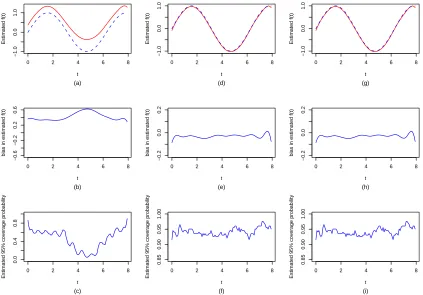
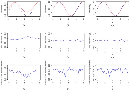
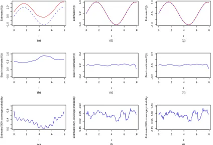
Figure 2.1 to 2.4 display and compare the estimated nonparametric function fb(t), its

empirical bias and point-wise 95% coverage probabilities of the true fixed function f(t)

across three methods for the different scenarios considered in this study. Figure 2.1 and 2.2

are generated from model (2.8) with data consisting of 17% and 34% censored observations

respectively. Figure 2.3 and 2.4 are generated similarly from model (2.9). It is clear that

in all cases, the naive imputation method produced significantly biased (upwards) estimate

b

f(t), leading to invalid confidence intervals for f(t) and yielding low coverage probabilities

for the confidence intervals. In contrast, both the direct optimization approach and the EM

algorithm produced virtually unbiased nonparametric function estimate fb(t) and correct

standard error estimates (results not shown). The coverage probabilities of the point-wise

Wald confidence intervals off(t) are close to the nominal level (95%) with slightly increased

fluctuation at the high censoring rate. Overall, there is no noticeable difference in the results

onf(t) between the direct optimization procedure and the EM algorithm. In summary, our

simulation demonstrates that SPMMs, coupled with the direct optimization procedure or

the EM algorithm, provide efficient parameter estimates and inference in the analysis of

(37)

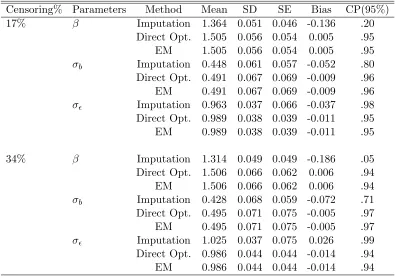
Table 2.1: Simulation results from model (2.8). Mean is the Monte Carlo mean of 200 estimates, SD is their Monte Carlo standard deviation, SE is the average of the 200 estimated standard errors, Bias is the difference between the mean estimates and true values and CP(95%) is the Monte Carlo coverage probability of the true parameter values based on 95% Wald confidence intervals.

Censoring% Parameters Method Mean SD SE Bias CP(95%)

17% β Imputation 1.364 0.051 0.046 -0.136 .20

Direct Opt. 1.505 0.056 0.054 0.005 .95

EM 1.505 0.056 0.054 0.005 .95

σb Imputation 0.448 0.061 0.057 -0.052 .80

Direct Opt. 0.491 0.067 0.069 -0.009 .96

EM 0.491 0.067 0.069 -0.009 .96

σ Imputation 0.963 0.037 0.066 -0.037 .98

Direct Opt. 0.989 0.038 0.039 -0.011 .95

EM 0.989 0.038 0.039 -0.011 .95

34% β Imputation 1.314 0.049 0.049 -0.186 .05

Direct Opt. 1.506 0.066 0.062 0.006 .94

EM 1.506 0.066 0.062 0.006 .94

σb Imputation 0.428 0.068 0.059 -0.072 .71

Direct Opt. 0.495 0.071 0.075 -0.005 .97

EM 0.495 0.071 0.075 -0.005 .97

σ Imputation 1.025 0.037 0.075 0.026 .99

Direct Opt. 0.986 0.044 0.044 -0.014 .94

(38)

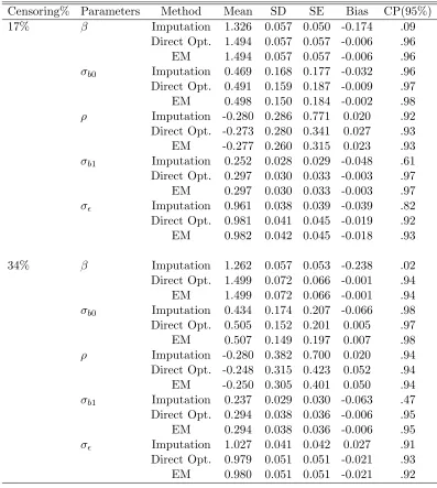
Table 2.2: Simulation results from model (2.9). Mean is the Monte Carlo mean of 200 estimates, SD is their Monte Carlo standard deviation, SE is the average of the 200 estimated standard errors, Bias is the difference between the mean estimates and true values and CP(95%) is the Monte Carlo coverage probability of the true parameter values based on 95% Wald confidence intervals.

Censoring% Parameters Method Mean SD SE Bias CP(95%)

17% β Imputation 1.326 0.057 0.050 -0.174 .09

Direct Opt. 1.494 0.057 0.057 -0.006 .96

EM 1.494 0.057 0.057 -0.006 .96

σb0 Imputation 0.469 0.168 0.177 -0.032 .96

Direct Opt. 0.491 0.159 0.187 -0.009 .97

EM 0.498 0.150 0.184 -0.002 .98

ρ Imputation -0.280 0.286 0.771 0.020 .92

Direct Opt. -0.273 0.280 0.341 0.027 .93

EM -0.277 0.260 0.315 0.023 .93

σb1 Imputation 0.252 0.028 0.029 -0.048 .61

Direct Opt. 0.297 0.030 0.033 -0.003 .97

EM 0.297 0.030 0.033 -0.003 .97

σ Imputation 0.961 0.038 0.039 -0.039 .82

Direct Opt. 0.981 0.041 0.045 -0.019 .92

EM 0.982 0.042 0.045 -0.018 .93

34% β Imputation 1.262 0.057 0.053 -0.238 .02

Direct Opt. 1.499 0.072 0.066 -0.001 .94

EM 1.499 0.072 0.066 -0.001 .94

σb0 Imputation 0.434 0.174 0.207 -0.066 .98

Direct Opt. 0.505 0.152 0.201 0.005 .97

EM 0.507 0.149 0.197 0.007 .98

ρ Imputation -0.280 0.382 0.700 0.020 .94

Direct Opt. -0.248 0.315 0.423 0.052 .94

EM -0.250 0.305 0.401 0.050 .94

σb1 Imputation 0.237 0.029 0.030 -0.063 .47

Direct Opt. 0.294 0.038 0.036 -0.006 .95

EM 0.294 0.038 0.036 -0.006 .95

σ Imputation 1.027 0.041 0.042 0.027 .91

Direct Opt. 0.979 0.051 0.051 -0.021 .93

(39)

0 2 4 6 8 −1.0 0.0 1.0 t Estimated f(t) (a)

0 2 4 6 8

−0.6

−0.2

0.2

0.6

t

bias in estimated f(t)

(b)

0 2 4 6 8

0.0

0.4

0.8

t

Estimated 95% coverage probability

(c)

0 2 4 6 8

−1.0 0.0 1.0 t Estimated f(t) (d)

0 2 4 6 8

−0.2

0.0

0.2

t

(e)

0 2 4 6 8

0.85

0.90

0.95

1.00

t

(f)

0 2 4 6 8

−1.0 0.0 1.0 t Estimated f(t) (g)

0 2 4 6 8

−0.2

0.0

0.2

t

(h)

0 2 4 6 8

0.85

0.90

0.95

1.00

t

(i)

Figure 2.1: Estimated nonparametric time function fb(t) (solid line) with the true fixed

function f(t) (dashed line) superimposed (top row panel), empirical biases of fb(t)

(mid-dle row panel) and pointwise 95% coverage probabilities of f(t) (bottom row panel) for

(40)

0 2 4 6 8 −1.0 0.0 1.0 t Estimated f(t) (a)

0 2 4 6 8

−0.6

−0.2

0.2

0.6

t

(b)

0 2 4 6 8

0.0

0.4

0.8

t

(c)

0 2 4 6 8

−1.0 0.0 1.0 t Estimated f(t) (d)

0 2 4 6 8

−0.2

0.0

0.2

t

(e)

0 2 4 6 8

0.85

0.90

0.95

1.00

t

(f)

0 2 4 6 8

−1.0 0.0 1.0 t Estimated f(t) (g)

0 2 4 6 8

−0.2

0.0

0.2

t

(h)

0 2 4 6 8

0.85

0.90

0.95

1.00

t

(i)

(41)

0 2 4 6 8 −1.0 0.0 1.0 t Estimated f(t) (a)

0 2 4 6 8

−0.5

0.0

0.5

1.0

t

Bias in estimated f(t)

(b)

0 2 4 6 8

0.0

0.4

0.8

t

(c)

0 2 4 6 8

−1.0 0.0 1.0 t Estimated f(t) (d)

0 2 4 6 8

−0.2

0.0

0.2

t

(e)

0 2 4 6 8

0.85

0.90

0.95

1.00

t

(f)

0 2 4 6 8

−1.0 0.0 1.0 t Estimated f(t) (g)

0 2 4 6 8

−0.2

0.0

0.2

t

(h)

0 2 4 6 8

0.85

0.90

0.95

1.00

t

(i)

(42)

0 2 4 6 8 −1.0 0.0 1.0 t Estimated f(t) (a)

0 2 4 6 8

−0.5

0.0

0.5

1.0

t

(b)

0 2 4 6 8

0.0

0.4

0.8

t

(c)

0 2 4 6 8

−1.0 0.0 1.0 t Estimated f(t) (d)

0 2 4 6 8

−0.2

0.0

0.2

t

(e)

0 2 4 6 8

0.85

0.90

0.95

1.00

t

(f)

0 2 4 6 8

−1.0 0.0 1.0 t Estimated f(t) (g)

0 2 4 6 8

−0.2

0.0

0.2

t

(h)

0 2 4 6 8

0.85

0.90

0.95

1.00

t

(i)