Mapping Quantitative Trait Loci for Complex Binary Diseases Using Line Crosses

(1)

Copyright 0 1996 by the Genetics Society of America

Mapping

Quantitative

Trait Loci for Complex Binary

Diseases Using Line Crosses

**Shizhong Xu* and William**

R. Atchleyt

*Department of Botany and Plant Sciences, University of Califvrnia, Riverside, California 92521-0124 and tDepartment of Genetics, North Carolina State University, Raleigh, North Carolina 27695-761 4

Manuscript received November 1, 1995 Accepted for publication April 3, 1996

ABSTRACT

A composite interval gene mapping procedure for complex binary disease traits is proposed in this paper. The binary trait of interest is assumed to be controlled by an underlying liability that is normally distributed. The liability is treated as a typical quantitative character and thus described by the usual quantitative genetics model. Translation from the liability into a binary (disease) phenotype is through the physiological threshold model. Logistic regression analysis is employed to estimate the effects and locations of putative quantitative trait loci (our terminology for a single quantitative trait locus is QTL while multiple loci are referred to as QTLs) . Simulation studies show that properties of this mapping procedure mimic those of the composite interval mapping for normally distributed data. Potential utilization of the QTL mapping procedure for resolving alternative genetic models (e.g., single- or two- trait-locus model) is discussed.

C

OMPLEX disease refers to any disease with unknown mode of inheritance, especially polygenic models. The genetic mechanisms underlying such complex diseases are usually analyzed using quantitative genetics techniques whose classical model partitions a complex trait into genetic and environmental compo- nents. The genetic component is thought to be controlled by a number of loci each with a small effect ( BULMER 1971; FALCONER 1981 )

.

Many disease-resistant traits in plants and animals are described as quantitative characters. For instance, resistance to Gibberella zeae infection in maize was measured as the ratio of the infected area to the total area in the inoculated internode ( PE et al. 1993), while resistance to blast fungus infection in rice was measured by lesion number and size ( WANG et al. 1994). Mapping genes for such quantitative disease traits can be accomplished by traditional interval mapping procedures (LANDER and BOTSTEIN 1989; HALEYand KNOTT 1992) and meth- ods of composite interval mapping (JANSEN 1993,1994; ZENG 1993, 1994).

Some disease-susceptible traits, however, are not quantitative characters, but rather are qualitative traits and usually binary response variables. The vast majority of qualitative disease traits have a polygenic basis, such as the fusiform rust disease resistance in loblolly pine where the trait is described as presence or absence of the formation of galls ( WILCOX 1995)

.

The genetic mechanism underlying rustdisease resistance in l o b lolly pine is still unknown. It is heritable but not inher-

Corresponding author: Shizhong Xu, Department of Botany and Plant Sciences, University of California, Riverside, CA 92521-0124. E-mail: [email protected]

Genetics 1 4 3 1417-1424 (July, 1996)

ited in a simple Mendelian fashion. It is not a single gene trait and environment also plays a role. Binary disease traits with a polygenic basis are also categorized as complex diseases.

WRIGHT (1934) proposed a “physiological threshold” theory to explain the link between a continuous latent variable and an observable binary phenotype. The threshold theory states that underlying the dichot- omy (phenotype)

,

there is a “scale of factor combina- tions” to which each factor (locus) makes a fairly constant contribution. More recently, this scale of factor combination (plus a random environmental deviation) was referred to as “liability” (e.g., FALCONER 1981 )

.

When liability is below the threshold an individual has the “normal” phenotypic expression, when it is above the threshold the individual has the “affected” phenotypic expression. Therefore, quantitative genetic analysis of a complex disease refers to the genetic study of the liability and the threshold.

Mapping genes for such binary traits is more compli- cated than that for continuous traits. Current methods are limited to analyses of the association between a marker and a quantitative trait loci (QTL) using a simple 2 X 2 chi-square test (e.g., WILCOX 1995). The chi- square test uses one marker at a time that does not provide estimates of the effect and position of the QTL. In addition, if multiple QTLs occur in the same linkage group, the chi-square test tends to be biased. HALEY and KNOTT ( 1992) suggest using generalized linear model approach to analyze such threshold traits. JANSEN

(2)

1418 and W. R.

ages. However, systematic investigation of gene mapping for binary traits under the physiological threshold model has been lacking. Herein, we modify the (composite) interval mapping procedures applied to continuous traits (LANDER and BOTSTEIN 1989; JANSEN 1993, 1994; ZENG 1994) to interval mapping for binary data.

MODEL OF LIABILITY

A complex disease trait is assumed to be controlled by a latent variable, referred to as liability, which is considered to be continuous and normally distributed. It can be described by the usual linear model

rn

z, =

4 +

b,xq

+ ei,

( 1 )

j = 1

where z, is the liability for the ith individual,

4

is the grand mean (intercept), xii is the j t h explanatory variable, b, is the regression coefficient and e, is the residual with a distribution of N ( 0, 0:). Since the liability is

unobservable, the mean and residual variance can be set at any arbitrary values. For simplicity, we choose

&,

= 0 and 0: = 1 throughout the presentation.

Our purpose is to map QTLs controlling disease trait using molecular markers, thus, the explanatory variables are now defined as indicator variables of marker genotypes. In fact, other fixed effects, such as sex, age and location of field, can be incorporated into the model to control the residual variance, but they are ignored here for convenience. Let us consider, for simplicity, a backcross population derived from two inbred parental lines, P1 and R2, fixed for alternative alleles at several QTLs and m markers. Let us assume that the backcross population is derived from Fl X PI so that a backcross individual can be either homozygous with Pl

allelic type or heterozygous with one Pl allele and one

P2 allele at a particular locus. If the ith individual is homozygous at the j t h marker, xil = 1, otherwise, xq = 0. The expected values of bj’s are given by ZENG ( 1993)

.

A disease susceptible trait ( y L ) , determined by the underlying liability, is a realized binary variable, defined as

Yz =

{

1 if affected

0 otherwise.

The device that translates liability into disease phenotype is the physiological threshold model (WRIGHT 1934). It assumes that there is a threshold ( 8 ) in the scale of liability, below which the individual has the normal phenotype, and above which it is affected. The translation can be summarized by

i

1 if zi 2 8 0 if zi

<

8

yi =

Estimation of regression coefficients requires the

conditional probability of yi = 1 given xi,’s, the marker genotypes. This conditional probability can be obtained by integrating out the random noise. Let us define z,

I X

as a conditional variable of

z,

given the QTL and marker genotypes. From model 1 we know that the conditional mean and variance are E ( zi

I

X ) = Cy=, b,x, and Var

( z ,

I

X ) = 1, respectively. We also know that the conditional variable is normally distributed because the residual term is assumed to be normal. Therefore, the den- sity function of the conditional variable is

The conditional probability of yt = 1 given X is ob-

tained by

where (a( [ ) stands for the standardized cumulative normal distribution function and [ is the argument. Analy- sis involving (a( < ) is referred to as probit analysis. We chose the probit model because the parameters are easy to interpret. However, the probit model is difficult to manipulate because numerical integration is required. So, a logistic model is employed to approximate (a(

E )

for estimation purpose. Logistic regressions have been used by human geneticists in segregation analysis (e.g.,

BONNEY 1986). The logistic model is expressed by

The approximate relationship between a probit model and a logistic model is Q, ([)

=

$( c[ ) , where c = 7r

/

6 .

Therefore,

This approximation is remarkably close when 0.1

<

a([)

<

0.9 (LIAO 1994). Hereafter, the probit model is replaced by its logistic approximation.

METHODS OF ESTIMATION

(3)

QTL Mapping for Binary Traits 1419

indicates linkage of the marker with a QTL. Let

p,

denote Pr

( y t =

l

I

X ) , then the log likelihood is

n n

L =

C

yz log(pi)

+

C

(1 - Y i ) lOg(1 -

pz).

( 4 )

i= 1 1=1

The unknown parameters are 8 and bj's, but 8 is a nui- sance parameter in linkage analysis and only 4 ' s are of interest. The maximum likelihood estimators are found by setting partial derivatives of L with respect to the parameters equal to zero. The first and second partial derivatives can be found in COX (1970). A statistical test for Ho:b, = 0 is carried out by the likelihood ratio (LR) approximation. The likelihood ratio test involves calculation of L under the full model, denoted by L 1 , and under the restricted model ( bJ = 0 ) , denoted by

I,,

.

The likelihood ratio is

-2

( 4, - L1 ) , which asymp- totically follows a chi-square distribution with one degree of freedom under the null hypothesis.

Standard computer programs for logistic regression analysis can be found in some commercial statistical packages such as PROC LOGISTIC in SAS (SAS Insti- tute 1988).

Interval mapping: The multiple logistic regression analysis provides a test for marker QTL association, but it does not give estimates of the size and location of a tested QTL. Assuming one QTL on a chromosome, LANDER and BOTSTEIN (1989) developed the interval mapping procedure, which can separate the QTL effect and the linkage parameter. Let us set the effect of the heterozygous genotype to zero and that of the homozy-

gous genotype to a for a particular QTL. Note that

arbitrarily setting the effect of the heterozygous genotype to zero does not change the estimation and test of the QTL effect, but it will affect the estimation of the threshold ( 0 ) . We describe the liability using the model of ZENG (1994) where an indicator variable represent- ing the QTL genotype is included in the model. His model is different from that of LANDER and BOTSTEIN

(1989) in that other important markers are incorporated as covariates to control the genetic background of other chromosomal regions. ZENG'S model is described by

z, = b*x,

+

4

xzl

+

e , , ( 5 )

where b* is the effect of a putative QTL ( 6 * = a ) in the tested interval, x? is an indicator variable represent- ing the genotype of the putative QTL,

f2

indexes the markers excluding the two flanking ones. Note that

x

:

is no longer known for sure and it takes a value of

1 or 0 with a probability depending on the genotypes of the two flanking markers and the QTL position. The conditional probability of x? = 1 is expressed by J = Pr ( x ? = 1

I

xil x i n ) , where x t l and . x z p are the indicators

of the two flanking marker genotypes. Let rl and r2 be the recombination fractions of the QTL with the left and the right markers, respectively, and denote the re-

j € S l

combination fraction between the two markers by r.

Without interference, the conditional probability of x? = 1 is ( DOERCE et al. 1994)

( 1 - r I ) ( 1 - - r 2 ) / ( l - ~ ) i f x z l = x i p = l

(1 - 7-1)?2/7. if xil = 1 and x t 2 = 0

r l ( 1 - % ) / r if xjl = 0 and xt2 = 1

~1r2/ ( 1 - r ) if xil = xt2 = 0.

Since the putative QTL is assumed to be inside the interval, r2 is a function of rl and r , as shown by

$ =

1

r 2 = - . ?" - q 1 - 2r1

It is taken that r is known, so that there is only one independent unknown recombination fraction.

The conditional probability of

y2

= 1 given the marker genotypes is partitioned into two parts,

p i l

and

pio.

If

x?

= 1, this probability is

p,

where

Logit(p,l) = LOg[p,l/(l - pi1)l

= ~ [ b * + b l ~ i i - d

.

( 6 )

j E I 1

1

= c[

c

4

XC! - 01

.

( 7 )

If

x?

= 0, the conditional probability becomes

pz(,,

where

Logit(pio) = LOg[p,o/ ( 1 - pia)

1

jEC2

The likelihood function becomes

n

L =

n

[Jp;?

( 1 - p j l ) l P V t

+

( 1 - J ) P ? o i= 1

x

( 1 -

**p * " ) L - J L**

( 8 )

whose solutions can be solved via the expectation-maximization ( E M ) algorithm. In this particular case, the EM algorithm requires the first and second partial derivatives of L with respect to the unknown parameters. These partial derivatives and the EM steps are given in the APPENDIX.

The unknown parameters are b*, 4 ' s and 8, but only

(4)

S. Xu and W.

30

25

20

K

A

10

5

n "

0 10 20 30 40 50 60 70 80 90 100

Testing Position (cM)

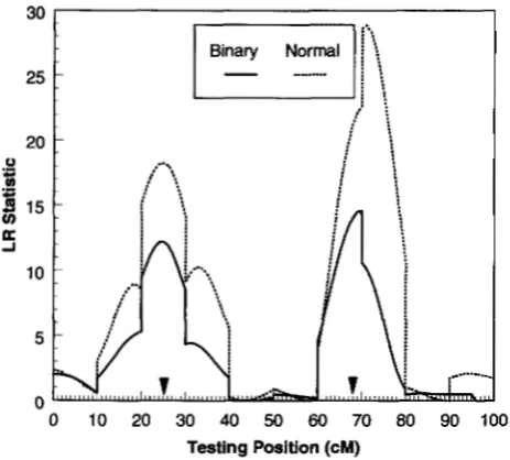
FIGURE 1.-Likelihood ratio profiles of interval mapping from one replicate of simulation in a backcross population of size 500. There are two QTLs located at 25 and 68 cM positions of the chromosomal segment. The solid curve repre- sents QTL mapping for binary data using the logistic regression presented in this paper. The dotted curve stands for QTL mapping for normally distributed data of the liability (as if it were the observed phenotype) using ZENG'S composite interval mapping.

SIMULATION

An example: To illustrate the properties of the method, a simulation study was performed. One chromosome with 11 markers separated in 10 10-cM inter- vals was simulated for a backcross population. The underlying liability is affected by two QTLs located in the positions of 25 and 68 cM (depicted in Figure 1 ) with gene effects of

a,

= 0.931 and a, = -0.931 units, respectively. Dominance and epistasis were assumed to be ab- sent. Using HALDANE'S mapping function, the recombination frequency between the two QTLs is r = 0.2884. The additive genetic variance is a i = [ a :

+

a;

+

2 ( 1

- 2r) a , c ~ ] / 4 = 0.25. The liability of each individual was generated by adding a random normal deviate, e

-

N ( 0, 1 )

,

to the additive genetic value. The mean and variance of the liability are Z = ( al

+

e)

/ 2 = 0.0

and 0 ; = 0;

+

a: = 0.25

+

1.0 = 1.25. Each QTL alone accounts for 17.34% of the total variation and the two QTLs jointly account for 20% of the total variation (due to a negative covariance between the two loci). To convert the continuous liability into a binary responsible variable, we set the threshold at 0 = 0.0, which leads to 50% of the individuals being affected. Sample size of this simulation was 500, which is suffi- ciently large to demonstrate the general properties of the method.

The data set generated under the genetic model described above was used for the composite interval m a p ping analysis. For comparison, the liability was treated as if it were the observed phenotypic variable and the

continuous data of the liability were analyzed using ZENG'S (1994) composite interval mapping procedure. Figure 1 shows the likelihood profiles from one replicate of the simulation. Both methods had successfully detected the two QTLs in the right locations. However, analysis of the binary data shows a lower profile than that of the normal data because some information has been lost when converting normal into binary data. A lower profile implies a lower statistical power. Similar results have been observed from analyses of more replicates (not shown).

Power studies: To compare the statistical powers and estimation errors of interval mapping for binary data with those for normal data, more simulations were con- ducted. One QTL located in the middle of a single interval of 20 cM was simulated. We considered the following factors that may have great influence on the performance of the mapping procedures: ( 1 ) sample size, ( 2 ) size of the QTL, and ( 3 ) threshold. Two levels were investigated for each factor and simulation was repeated 100 times in each parameter combination. The effect of the QTL was set at a = 0.459 and 0.667, corresponding to h' = 0.05 and 0.10, respectively. The threshold determines the proportion of disease infection (disease incidence) and it was set at values such that the disease incidences were at 25 and 50%. A criti- cal value of 3.84 (the critical value at a = 0.05 of the

x'

distribution with one degree of freedom) in the test statistic was chosen to determine the statistical powers. The actual critical value may be slightly higher than 3.84 ( HALEY and KNOTT 1992). Results are given in Table 1 and Table 2 for situations where disease incidences are 50 and 25%, respectively. In general, the gene mapping procedure for binary data performs very well. Compared with the analyses when the liability is treated as if it were observed normal phenotype, the binary method has lower power and larger estimation error, especially when the disease incidence deviated from 50%. Note that the logistic regression approximation requires that the disease cannot be too rare, else the approximation does not hold.

DISCUSSION

(5)

QTL Mapping for Binary Traits

TABLE 1

Statistical powers and estimation errors when the disease incidence (proportion of affected individuals) is about 50%

Sample Data Test

Heritability" size w e cMAh ri" statistic Power (%)"

0.05 200 Binary _{9.79 (7.616)} _{0.42 (0.19)} _{7.33 (5.74)} ₆₄

Normal 9.34 (7.13) 0.46 (0.16) 10.36 (6.59) 87

500 Binary _{10.25 (6.29)} _{0.39 (0.11)} _{13.69 (7.05)} ₉₈

Normal _{9.95 (4.97)} _{0.46 (0.09)} _{22.02 (8.42)} ₁₀₀

Normal _{10.00 (4.64)} _{0.71 (0.15)} _{20.94 (8.27)} ₁₀₀

500 Binary _{9.92 (4.37)} _{0.60 (0.11)} _{28.17 (10.08)} ₁₀₀

Normal _{10.20 (3.53)} _{0.67 (0.10)} _{44.47 (12.29)} ₁₀₀

0.10 200 Binary 9.86 (5.52) 0.63 (0.17) 13.11 (6.16) 96

The table shows the average estimates and standard deviations (in parentheses) from 100 replicates of simulation.

Proportion of the total variation in liability explained by the QTL. bEstimated position of the QTL. The parametric value is 10 cM. 'Estimated effect of the QTL.

"

Statistical power at an error rate of 0.05.

1421

hood is used for the logistic regression analysis. Proper- ties of this mapping technique resembles those of the composite interval mapping of ZENG ( 1994) for normal data.

The interval mapping procedure for binary traits is usually less powerful than the well developed mapping methods for continuous traits. This is because some information will be lost during the translation from the underlying liability into the observed binary phenotype. The threshold

( e )

is the leading parameter that determines the amount of information loss. The threshold determines the disease incidence (proportion of infected individuals) in the population of interest. The efficiency of the interval mapping largely depends on the disease incidence. The maximum efficiency occurs when the disease incidence is 50%. Consider that statistical power is a monotonically increasing function of the heritability of the putative. This heritability has a maximum value when the disease incidence is 50% (ED- WARDS 1969). As the disease incidence deviates from

50%, more information will be lost. As a consequence,

the method presented here is not applicable to gene mapping for rare diseases. Although f3 cannot be controlled in natural populations, it can be manipulated in designed experiments. In QTL mapping experiments, plants are usually artificially inoculated by spraying a certain amount of pathogen spore suspension. Under some circumstances, one may adjust the amount of spore suspension to make the disease incidence close to 50% as much as possible.

Usually, the mechanisms underlying complex binary disease traits are not known. The physiological threshold model is only a hypothesis that is hardly tested. However, a plausible biological interpretation of the threshold model can be drawn from the threshold char- acteristic of enzyme activity. MOZHAEV et d . (1989)

found that the dependence of the catalytic activities of a-chymotrypsin and lactase on the concentration of organic cosolvents in mixed aqueous media has a pro- nounced threshold character: the activity does not change up to a critical concentration of the nonaque- ous cosolvents added, yet further increase of the latter

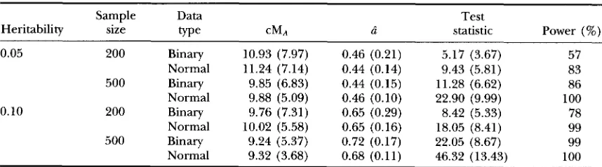
TABLE 2

Statistical powers and estimation errors when the disease incidence (proportion of affected) is 25%

Sample Data Test

Heritability size w e CMA d statistic Power (%)

0.05 200 Binary _{10.93 (7.97)} _{0.46 (0.21)} _{5.17 (3.67)} ₅₇

Normal _{11.24 (7.14)} _{0.44 (0.14)} _{9.43 (5.81)} ₈₃

500 Binary _{9.85 (6.83)} _{0.44 (0.15)} _{11.28 (6.62)} ₈₆

Normal _{9.88 (5.09)} _{0.46 (0.10)} _{22.90 (9.99)} ₁₀₀

Normal _{10.02 (5.58)} _{0.65 (0.16)} _{18.05 (8.41)} ₉₉

500 Binary _{9.24 (5.37)} _{0.72 (0.17)} _{22.05 (8.67)} ₉₉

Normal _{9.32 (3.68)} _{0.68 (0.11)} _{46.32 (13.43)} ₁₀₀

0.10 200 Binary 9.76 (7.31) 0.65 (0.29) 8.42 (5.33) 78

(6)

S. W.

(by only a small amount) leads to an abrupt decrease in enzyme activity. Consider that disease resistance is determined by the activity of a particular enzyme. The locus coding for this enzyme may be called the major gene. In a population where the major gene has been fixed, the disease phenotype may still show polymor- phism. This may occur when the enzyme activity is determined by the level of gene products of several QTL. The collective effect of the gene products of the QTLs is analogous to the liability. When the level of the gene products reaches a certain threshold, the enzyme becomes inactive, leading to disease infection.

A well-known alternative to the threshold model is that the expression of a disease trait is determined by the expression of one or two loci ( SCHORK 1993)

.

If the disease in question is controlled by one locus and environment does not play a role, the disease expression in a backcross population will show simple Mende- lian segregation. In this case, there is no need to invoke the threshold model of gene mapping. However, the threshold model is appropriate in dealing with situations where the disease is controlled by a single locus but environmental effect also plays a role in the expression of the disease trait. In genetic mapping of diseases under one- or two-locus model, the conditional probability of trait expression of a given genotype is usually referred to as penetrance ( SCHORK 1993). For example, the penetrances of homozygotes ( x * = 1 ) and heterozygotes (x* = 0 ) in a backcross population are denoted by

p l = P r ( y = l I x * = l ) and p , = P r ( y = l I x * = O ) ,

respectively. It is then natural to use the difference between

pl

and

P,

to detect the effect of the putative locus on the disease. Recall that

x* is unobservable but

its

conditional distribution given marker genotypes is known (denoted by J )

.

Therefore, the log likelihood function can be constructed as

n

i= 1

+

( 1 -&)$I&( 1 - p o ) "yt].

The maximum likelihood extimates of

pl

and

Po

are solved iteratively by

n

i= I i= 1

where

Under the null hypothesis Ho:

pl

= =

p ,

the log likelihood function becomes

As

usual, the likelihood ratio statistic is used to test the null hypothesis.

We now show that the above test is equivalent to that under the threshold model. When the expression of a disease trait is determined by a single locus, it is not necessary to include nonflanking markers in the model of liability. Thus, the penetrance can be expressed as

when x* = I, and

when x* = 0. Instead of maximizing the log likelihood function with respect to

pl

and

Po,

we now maximize the likelihood with respect to b* and B ( cis a constant)

.

According to the invariance property of the maximum likelihood method ( DEGROOT 1986), the maximum likelihood estimates of

9

and b* are

e

= - - 1 l o g [ j o / ( l - i o ) ]

c

and

respectively. Clearly, the null hypothesis that b* = 0 is equivalent to that

pl

=

Po.

When the disease is controlled by two loci and environment plays a role in the expression of disease trait, the threshold model proposed in this paper is still valid as long as there is no epistatic interaction between the two loci. In the presence of epistatic effect, the current threshold model must be modified so that two QTLs are mapped simultaneously using a two-dimensional search strategy (e.g., HALEY and KNOTT 1992), an area that deserves further investigation.

(7)

QTL Mapping for Binary Traits 1423

there are several thresholds to translate the liability into

observed ordinary disease phenotypes ( LANGE et al.

1976). The binary data analysis will be a special case of

the general procedure for ordinary data analysis for

which further investigation is required.

This work was supported by National Research Institute Competi- tive Grants Programs/U.S. Department of Agriculture 95-37205-2313

to S. X. and National Institutes of Health grant GM45344 and Na- tional Science Foundation BSR-910718 to W. R. A.

LITERATURE CITED

BONNEY, G. E., 1986 Regressive logistic models for familial disease and other binary traits. Biometrics 4 2 61 1-625.

BULMER, M. G., 1971 The effect of selection on genetic variability.

A m . Nat. 104 201-211.

CHURCHILL, G. A,, and R. W. DOERGE, 1994 Empirical threshold values for quantitative trait mapping. Genetics 138: 963-971.

Cox, D. R., 1970 The Analysis of Binaly Data. Methuen & Co. Ltd., London.

DEGROOT, M. H., 1986 Probability and Statistics, Ed. 2. Addison-Wes- ley Publishing Co., Reading, MA.

DOERGE, R. W., Z.-B. ZENG and B. S. WEIR, 1994 Statistical issues in the search for genes affecting quantitative traits in populations, pp. 15-26 in Analysis ofMokcular MarkerData, Proceedings ofJoint

Plant Breeding Symposia Series, Corvallis, OR.

EDWARDS, J. H., 1969 Familial predisposition in man. Brit. Med. Bull. 25: 58-63.

FALCONER, D. S., 1981 Introduction to Quantitative Genetics, Ed. 2,

Longman, New York.

HALEY, C. S., and S. A. KNOTT, 1992 A simple regression method for mapping quantitative trait loci in line crosses using flanking markers. Heredity 69: 315-324.

JANSEN, R. C., 1992 A general mixture model for mapping quantitative trait loci by using molecular markers. Theor. Appl. Genet.

JANSEN, R. C., 1993 Interval mapping of multiple quantitative trait loci. Genetics 135: 205-211.

JANSEN, R. C., 1994 Controlling the Type I and Type I1 errors in mapping quantitative trait loci. Genetics 138: 871-881.

JANSEN, R. C., and P. STAM, 1995 High resolution of quantitative traits into multiple loci via interval mapping. Genetics 136: 1447-

1455.

LANDER, E. S., and D. BOTSTEIN, 1989 Mapping Mendelian factors underlying quantitative traits using RFLP linkage maps. Genetics

LANGE, K., J. WESTLAKE and M. A. SPENCE, 1976 Extensions to pedi- gree analysis: 11. Recurrent risk calculation under the polygenic threshold model. Hum. Hered. 2 6 337-348.

LIAO, T. F., 1994 InterpetingProbability Models: Logzt, Probit, and Other

Generalized Linear Models. Sage University Paper series on Quanti-

tative Applications in the Social Sciences, 07-101. Thousand Oaks, CA.

MOZHAEV, V. V., Y. L. KHMELNITSKY, M. V. SERGEEVA, A. B. BELOVA, N. L. KLYACHKO et al., 1989 Catalytic activity and denaturation of enzymes in water/organic cosolvent mixtures. Eur. J. Bio- chem. 184: 597-602.

PE, M. E., L. GIANFRANCESCHI, G . TARAMINO, R. TARCHINI, P. ANGELINI et al., 1993 Mapping quantitative trait loci (QTLs) for resistance to Gibberella zeue infection in maize. Mol. Gen. Genet. 241:

11-16.

SAS INSTITUTE INC., 1988 SAS/STAT User's Guide, Release 6.03

Edition. SAS Institute Inc., Cary, NC.

SCHORK, N. J., M. BOE:HNKE, J. D. TERWILLIGER, and J. Om, 1993

Two-trait-locus linkage analysis: A powerful strategy for mapping complex genetic traits. Am. J. Hum. Genet. 5 3 1127-1136. WANG, G.-L., D. J. MACKILL, M. BONMAN, S. R. MCCOUCH, M. C.

CHAMPOUX et al., 1994 RFLP mapping of genes conferring com- cultivar. Genetics 136: 1421-1434.

plete and partial resistance to blast in a durably resistant rice

WILCOX, P. L., 1995 Genetic Dissection of Fzlsifonn Rust Resistance in

Loblolly Pine. Ph.D. Dissertation, Department of Forestry, North

Carolina State University, Raleigh.

85: 252-260.

121: 185-199.

WRIGHT, S., 1934 The results of crosses between inbred strains of guinea pigs differing in number of digits. Genetics 19: 537-551.

ZENG, Z.-B., 1993 Theoretical basis for separation of multiple linked gene effects in mapping quantitative trait loci. Proc. Natl. Acad. Sci. USA 90: 10972-10976.

ZENG, Z.-B., 1994 Precision mapping of quantitative trait loci. Genet- ics 136: 1457-1468.

Communicating editor: M. LYNCH

APPENDIX

This appendix gives the partial derivatives of the log likelihood function with respect to the unknown parameters and describes the EM steps.

Let x i o = - 1 for

i

= 1,

. . .

,

n and

j

indexes the

threshold (when

j

= 0, bj = 6 ) and all other markers

excluding the two flanking ones, then

and

The log likelihood function is n

L = log

[ $ p 3

( 1 - pil) l - x

i= 1

+

( 1 - ~ ) p j t , ( 1 - p i o ) " y ~ I *

The first partial derivatives are

and

for j = 0,

. . .

,

R,

where

$p;l ( 1 -

pil)

( l - x )

w.

=

'

&p?$

( 1 - pi1) ('-'*)

+

( 1 -

$)p{t,(

1 -

pEo)

(I-';)

is the posterior probability of x* = 1.

The second partial derivatives are messy because wi

is a function of the unknown parameters. However, if

these w,'s are treated as constants, then the second

partial derivatives have simple forms as shown:

d 2 L

db*

n

"

-

- c 2 C

WiPzl(1 - p i l ) ,

(8)

1424 S. Xu and W.

and

+

( 1 - ~ ) p i 0 ( 1 - p i ~ ) l x y x t k

f o r j , k = 0 , .

. .

, R

The EM steps are as follows

1. Set up initial values of b* and bj for j = 0 ,

. . .

,

a;

2.

Calculate w, (E-step) ;

3. Given w , , solve for b* and

4

using the NEWTON-

RAPHSON iteration ( "step ) ;

4.

Update the initial values and go to step 2 ) ; 5. Repeat steps

2-4

until convergence.

The maximization step is accomplished via the NEW- TON-RAPHSON iteration, which is described as follows. Let d be a vector of the first partial derivatives and J be a matrix of the second partial derivatives. If

p(

t ) is a vector of solutions at the tth step, the solutions at the

t

+

1 step is

p(

t

+

1 ) =

p(

t ) - J"d, where J and d are evaluated at

p(

t )