Using differences across US states to think
about consumption
Charles Grant
Septem ber 2001
A Thesis Submitted for the Degree of Doetor of Philosophy to University College London,
ProQuest Number: U642440
All rights reserved
INFORMATION TO ALL USERS
The quality of this reproduction is dependent upon the quality of the copy submitted. In the unlikely event that the author did not send a complete manuscript and there are missing pages, these will be noted. Also, if material had to be removed,
a note will indicate the deletion.
uest.
ProQuest U642440
Published by ProQuest LLC(2015). Copyright of the Dissertation is held by the Author. All rights reserved.
This work is protected against unauthorized copying under Title 17, United States Code. Microform Edition © ProQuest LLC.
ProQuest LLC
C ontents
A b stra ct vii
A ck now ledgem en ts viii
D ecla ra tio n ix
1 Introduction: 1
2 D a ta D escription: 6
3 B an k ru p tcy Law, C redit C onstraints and Insurance: Som e E m pirics 9
3.1 In tro d u c tio n ... 10
3.2 T h e o ry ... 12
3.3 Personal Bankruptcy in the United S t a t e s : ... 18
3.3.1 State Exemptions: 19
3.4 D ata D escrip tio n :... 26
3.5 R eg ression s:... 28
3.5.1 R e s u l t s : ... 28
3.5.2 C o n su m p tio n :... 32
3.6 C o n c lu s io n :... 35
3.7 A p p e n d i x ... 37
4 R isk Sharing and th e Tax S ystem 45 4.1 In tro d u c tio n ... 46
4.2 Taxes and Transfers... 48
4.3.1 Q uadratic U t i l i t y ... 52
4.3.2 Alternative Utility Specifications ... 53
4.3.3 The regression... 57
4.4 D a t a ... 59
4.4.1 Measuring Tax P rogressivity... 62
4.5 R e s u lts ... 64
4.6 C o n c lu sio n s ... 68
5 E stim a tin g C redit C onstraints am ong U S households. 80 5.1 In tro d u c tio n ... 81
5.2 The Literature On Credit Constraints... 82
5.3 An Empirical Fram ew ork... 88
5.3.1 Estim ation by Maximum L ik e lih o o d :... 90
5.4 D ata D escrip tio n :... 93
5.5 Results: ... 95
5.6 Conclusion: ... 101
List o f Tables
3.1 Expected effect of increasing the punishment for default. . . . . 18
3.2 Federal exemptions for Chapter 7 bankruptcy. 20 3.3 W hether, and in which year, the state passed legislation to not allow the federal exemptions to be claimed... 23
3.4 The level of exemptions (in dollars) over the sample period. 25 3.5 Summary statistics for different exemption quartiles... 27
3.6 Results of a tobit regression on household debt (probability in parentheses). 38 3.7 Results of a tobit regression on household debt, including state dummies (probability in parentheses)... 39
3.8 Results of a linear regression on the interest rate th a t the household pays (probability in parenthesis)... 40
3.9 Results of a linear regression on the interest rate th a t the household pays, including state dummies, (probability in parenthesis)... 41
3.10 Results of a linear regression of the growth rate of consumption (probability in parentheses)... 42
3.11 Results of a linear regression of the growth rate of consumption when state effects are included (probability in parentheses)... 43
3.12 Regressing Av ar {cu) against the bankruptcy exemptions... 44
4.1 Thresholds for current federal tax b r a c k e ts ... 71
4.2 Proportion paying at each marginal federal tax rate for 1982-1998 ... 72
4.3 State Individual Income Tax Rates in the US in 1999 73 4.3 (cont.) State Individual Income Tax Rates in the US ... 74
4.4 The level of transfers in the US 1982-1998 ... 75
4.5 Measuring tax p ro g re s s iv ity ... 75
4.6 Regressing A^sd^ (cit) against the mean tax rate (standard errors in paren theses)... 76
4.7 Regressing Asd^ (lnc*^) against the mean tax rate (standard errors in paren theses)... 76
4.9 Regressing (InQ^) against the (standard errors in parentheses). . . . 78
4.10 Estimated parameters in the insurance function 0 (r) — 1 — ao — aiT from
tables 4.7 and 4.9... 79
5.1 When US states deregulated and relaxed state banking regulations... 107 5.2 Some summary statistics on debt-holding among US households... 108
5.3 Estimated debt equations, in $l,000’s (standard errors in parentheses). . . . 109
List of Figures
3.1 The feasible region for debt holdings when the utility function has the form u (ci, di, C2, (^2) = In Cl + In di + /? In C2 + /51n ^2- Default is assured below the line... 16
4.1 The evolution of uar-^ (cjt)... 60
A bstract
This thesis investigates some contemporary issues in consumption using household data. It
exploits state of residence information available over several years using the Consumer Ex
penditure Survey: a US survey of spending, and a variety of other household characteristics.
The thesis contains three distinct studies. The first looks at how consumer bankruptcy rules
affects the debt holdings, and consumption behaviour of US households. Harsher punish
ment results in more debt but less smoothing. The second study looks at how differences
in state taxes translates into differences in the ability of agents to share the idiosyncratic
component of their income shocks, finding th a t making taxes more re-distributive reduces
agents ability to insure risks. The last study accepts th at some agents are credit-constrained,
and recovers estimates of the supply of, and the demand for, credit. This leads to estimates
of the proportion of agents credit constrained, 28%, of how agents differ, and of how much
A cknow ledgem ents
I would like to thank the many people whoe comments and advise helped to improve this
work. These included Orazio Attanasio, Erich Battistin, Gabriella Berloffa, Nick Bloom,
Chris Carroll, Vassilis Hajivassiliou, Christos Koulovatianos, Tullio Jappelli, Nick Souleles,
Mario Padula, Luigi Pistaferri, Ian Preston, Oved Yosha as well as several seminar partici
D eclaration
No part of this thesis has previously been presented to any University for any degree.
C h a p ter 1
Introduction:
This thesis explores some contemporary issues in consumption. Modern work on consump
tion started with the seminal paper by Hall (1978).^ This paper assumed quadratic and time
separable utility functions and explored the implications of the permanent income hypothe
sis. He developed an Euler equation th a t he then tested, and rejected, using US aggregate
data. Consequently, much of the next 15 years was spent testing various developments of
this basic formulation. Nevertheless, subsequent studies confirmed Hall’s result: changes in
income are over-sensitive to predictable changes in income, the excess sensitivity highlighted
by Flavin (1981), and changes too little in response to unpredictable income shocks, the
excess smoothness of, for instance Campbell (1987). Simple life-cycle models of consump
tion have also been rejected: Carroll and Summers (1991) shows how even over the whole
life-cycle th a t income and consumption seem to follow each other.
A number of explanations have been offered. Many studies have suggested alternative
utility functions, such as iso-elastic or log utility, and have allowed life-cycle or preference
parameters to enter the utility function. If such utility functions are chosen, then aggregate
data is no longer appropriate. Attanasio and Weber (1993) showed th a t using micro-data
and explicitly controlling for taste shifters at the household level could account for much
of the variation in consumption. Nevertheless, it is not believed th a t tastes-shifters, such
as family size, can itself explain all of the rejection of the Euler equation first highlighted
by Hall. Instead two other possible explanations have been popular. One idea is th at if
the agent is risk-averse, then there will be a precautionary motive to saving. Indeed, if
agents are risk-averse, prudent and cautious, in the sense described by Zeldes (1989), then
in a remarkable paper Carroll (1997) dem onstrated th a t this itself could cause income and
consumption to track together over the life-cycle. The second popular explanation is th at at
least some households are sometimes credit-constrained. Households would like to borrow
against their future income, and thus smooth consumption, but for some reason they are not
allowed to borrow as much as they would like at the prevailing interest rate. In practise, this
different explanations are difficult to convincingly distinguish, at least with the kind of data
consumption economists have hitherto used. The problem is th a t the different explanations
have few, if any, observational implications th a t differ between the explanations.
Much of the more recent consumption literature has instead looked at risk-sharing across
states of nature. One implication the complete market hypothesis is th a t agents should be
able to pool their risks, and thus only aggregate risk, and not idiosyncratic risk, should
enter into changes in consumption. This was first tested by Mace (1991), and, as might be
expected, was rejected. Nevertheless, the study of risk-sharing has given some important
insights. In particular, the theoretical literature, in such papers as Kehoe and Levine (1993)
or Kocherlakota (1997) has stressed th a t risk-sharing is limited since agents will only credibly
commit to sharing their income when they have good draws from nature if they are sufficiently
compensated, or face an environment th a t is sufficiently risky, when they have bad income
draws. Otherwise, they will not lend regardless of the interest rate. In other words, such
models endogenously create credit-constraints, and such constraints are intimately related
study in the thesis. This chapter investigates how the default rules, th a t is the rule about how
the debtors assets are shared between the borrower and lender when the debtor defaults,
affects the amount of debt th a t debtors hold. Intuitively, one would expect th a t harsher
rules will allow more debt to be held in equilibrium: a result confirmed by this study. One
problem is th a t it then seems optimal to punish default with an arbitrarily large punishment.
One possible explanation of arbitrarily large punishments are not observed might be th at
allowing default in ex post bad income realisations may insure the agent against bad income
shocks. Hence this study also looks at the insurance effect of the default rules, and finds
weak evidence to support the proposition th at harsher rules provide less insurance since more
of the risk of bad income realisations is borne by the debtor in this case.
The problem of risk-sharing is more directly analyzed in the fourth chapter. So far the
empirical literature has noted th a t full insurance can be rejected by the data. However,
full insurance seems a wholly implausible hypothesis, and it is hardly surprising th a t this
model is rejected. However, the tests th at have been constructed are not fully constructive:
they do not help us to understand either how much insurance is available to agents, or
what factors may contribute to the overall level of insurance. Chapter 4 concentrates on
exactly this problem. It will formulate a measure of risk-sharing th a t can be related to some
policy instrument. The chapter attem pts to explain how the amount of extra insurance a
particular policy instrum ent gives. The policy instrument th a t the chapter investigates is
the tax system: the study measures how much extra risk-sharing occurs when taxes become
more redistributive, i.e. for a fixed total tax revenue, how the distribution of tax liabilities
between rich and poor changes the extent to which agents can smooth consumption against
states of nature. As will be seen, the study reaches a surprising conclusion.
Chapter 5 takes as given th a t at least some agents are credit constrained. Chapter 3
found th a t borrowing was related to the punishment for default, hence this might not be too
of desired borrowing (demand) and the maximum level of borrowing th a t any lender will
allow (supply). Only this minimum is generally observed and it is not usually known whether
the agent wished to borrow more than this observed amount. Chapter 4 explains how to
separately recover both supply and demand as long as exclusion restrictions can be made:
things th at enter supply and not demand, and things th a t enter demand and not supply.
The plausibility of the results depends crucially on the ability to find appropriate exclusion
restrictions. The approach, as will be explained, builds on the literature on disequilibrium
models.
The main body of work is contained in chapters 3 to 5. Most consumption literature has
focused on changes over time, either looking at aggregate time series, or looking at synthetic
cohorts in which identification is through a large number of time series. Instead this thesis
will exploit differences across the environment in which agents reside. In fact, it is difficult to
know how the issues addressed in this thesis could convincingly be studied in any other way.
The difference th at is exploited is th at different agents reside in different US states. These
US states differ in the their regulations on bankruptcy regulations (exploited in chapter 3),
in their tax systems (exploited in chapter 4), and in their banking regulations (exploited in
chapter 5). However, unlike a comparison across countries, states and the individuals in the
states are still fairly homogeneous. For instance, the law regarding bankruptcy only differs
between states in regulating which assets may be kept when an agent becomes bankrupt:
all other regulations regarding bankruptcy are fixed across states. It also seems reasonable
to suppose attitudes towards risk, and towards default are similar across US states in a way
th a t they might not be across, say, OECD countries.
This thesis is able to exploit differences across states since it uses the Consumer Expendi
ture Survey. State data is available for 1980-1998 using this d ata set, something th at is fairly
unique for data. Chapter 2 starts with a brief description of this data set. Chapter 3 studies
4 looks and risk-sharing in more detail, and investigates whether the tax system helps agents
to smooth against their idiosyncratic risks. Chapter 5 looks at credit constraints, and the
C h a p ter 2
D a ta D escription:
Since the empirical research contained in the different chapters of this thesis exploits the US
Consumer Expenditure Survey (henceforth the CEX), this chapter gives a brief explanation,
and discussion of those aspects of the data th at are common between the different chapters.^
The CEX is a consumer survey of households th a t is available on a continuous basis since
1980. The survey is conducted by the Bureau of Labor Statistics in the US and was origi
nally designed to construct a measure of inflation. As a result a large number of households,
around 7,000 each quarter, are asked to respond to extremely detailed questions about cur
rent spending, as well as being asked about a variety of demographic and other household
characteristics. Households are interviewed 5 times; the first being a contact interview (from
which no information is disclosed); and four subsequent interviews at 3 monthly periods. The
survey is constructed as a rotating panel, hence each quarter, one fifth of the households
having reached their fifth interview drop out and are replaced. In each interview households
recall their household expenditures in each of the previous three months. However, since
many households, for many expenditure items, have assigned to them the same expenditure
to each of the three months, only the last of these three months will ever be considered.
Information is also recorded on income, although (unless the householder has changed em
ployment) this information is only asked in the second and fifth interview. A large number of
demographic and other household characteristics are recorded, including state of residence,
although for reasons of confidentiality this information is sometimes suppressed. The fact
th a t state information is available will be consistently exploited in this thesis.
From 1988 the survey has also included additional information on the households debts
in the second and fifth interviews. This information is used to construct the to tal unsecured
debts held by the household, including debts held in revolving credit accounts (including
store, gasoline, and general purpose credit cards), in installment credit accounts, credit at
banks or savings and loan companies, in credit unions, at finance companies, unpaid medical
bills, and other credit sources. It also includes negative balances held in checking or brokerage
accounts. Excluded from the total are mortgage, and other secured debts. This data will be
used in two of the chapters of this thesis.
Throughout this work, income, debt and exemption values will be deflated by the CEX
price index so th at they are in real terms. The price index is constructed aa a Stone-Geary
price index for individual households. This work will consistently exclude farming and self-
employed households. Also excluded are large households with eight or more members, and
households in which the respondent answers th a t they have received no education. Large
households are excluded because as the household becomes larger it becomes increasingly
problematic to describe the household’s characteristics by the characteristics of the household
head. Those households with heads who did not go to school may have poorer responses to
the survey. In any case, the number of households in these two categories was small. Other
excluded observations will be highlighted in the chapter for which the exclusion is relevant.
Using the CEX has a number of advantages vis-a-vis other possible data sources. Unlike
the PSID, for instance, a large part of the households consumption can be reliably calculated.
consumption varies much less than total non-durable consumption in response to income
shocks. Furthermore, the CEX surveys many more households. The disadvantage is th at
the furthest apart any two observations can be is 9 months. A second problem is th at
household responses are based on recall data, rather than a diary (the construction of the
British Family Expenditure Survey, for instance). Never-the-less, it is not believed th a t this
is too serious a drawback.
The last and most im portant advantage is th a t the CEX contains information on state
of residence. Coupled with the large sample size, this has allowed this work to exploit the
differences between US states to measure some of the consumption effects th a t could not
be assessed in any other way. The only other data source for much of the information used
in this thesis is the Survey of Consumer Finances (SCF) which contains information on
household assets and debts th a t will be exploited in two of the chapters of this thesis. One
problem with this survey is th a t state information is only contained in the 1983 wave of the
data. A further problem is th a t th at data set has many fewer observations. Overall, the
CEX seems to be the dataset th at can best be used to explore some of the issues that I hope
C h a p te r 3
B ankruptcy Law, Credit C onstraints
and Insurance: Som e Em pirics
A b stra ct
Bankruptcy (defaulting on one’s debts) acts as insurance if it allows default in cases of
negative income shocks. However, whether bankruptcy provides insuranee depends on the
bankruptcy rules (the punishment for default) th a t is enforced. Bankruptcy rules can instead
cause the consumer to be credit constrained. If debts are not fully enforceable, a rational
lender may limit how much debt any borrowers are allowed to hold. This limit increases as
the punishment for defaulting increases. The US provides a natural test of the theory since
rules about which assets may be kept by the debtor, the state exemptions, when filing for
bankruptcy differ dramatically across the different states. Regressions show th a t increasing
the level of these exemptions causes less debt to be held by consumers. The chapter also
tests the theory more indirectly by regressing changes in the level, and in the variance, of
3.1
In tro d u ctio n
In recent years, a great deal of attention by consumption economists has been devoted to
the observation th a t consumption and income seem to follow each other, both over the
comparatively short intervals^ and over the whole lifecycle. Consumers seem to consume
more in the middle of their life, in their 40’s and 50’s, than either at the beginning or at
the end of their life. Carroll and Summers (1991) have shown how income and consumption
seem to track each other over the life-cycle. Several explanations have been suggested in the
literature, two of the most popular are: (1) households are risk averse, prudent and impatient
in the sense of Zeldes (1989) and Carroll (1997); and (2) households are credit constrained
and can not borrow, Deaton (1991). However, it has been difficult to distinguish the relative
importance of these different explanations. This chapter will use bankruptcy legislation as
an instrum ent th a t can shed light on these theories.
In a parallel literature, see Jackson (1986), bankruptcy rules have been motivated, partic
ularly among lawyers, as a device th at creates insurance when agents face uncertainty about
the future. At the same time a theoretical literature has attem pted to explain the fact th at
consumers can not fully insure all their idiosyncratic risk. Papers such as those by Kehoe
and Levine (1993) and Kocherlakota (1996) argue th a t this limited insurance is due to the
fact th a t debts can not be fully enforced.^ In such a framework, as shall be shown in section
3.2, the presence of a bankruptcy law which limits the punishment for default, may instead
create credit-constraints. One aim of this chapter is to bring together these two literatures,
and to empirically test what effect bankruptcy rules may have.
In the literature on risk-sharing, any mean preserving action th a t reduced uncertainty
^See, for example, Hall (1978)
will be welfare improving. Bankruptcy legislation can reduce uncertainty if the consumer can
default on his debt when his income is low. For bankruptcy legislation to act as insurance,
actually defaulting must be negatively correlated with income.^ Bankruptcy legislation can
have very different or even perverse effects if this is not the case. Section 3 starts with a
very simple discussion of how the penalty^, or sharing rule (how much the creditor and the
debtor each receive when the debtor defaults) affects the debtor’s incentives to default.
The punishment for debt differs across the different states of the United States quite
substantially, as, when defaulting, different levels of assets can be kept in different states.
Borrowers are assumed to be otherwise identical, and lenders face no constraints as to which
state they will lend in. An identifying assumption of the paper is th a t any other differences
in the operation of credit markets across the different states is orthogonal to the bankruptcy
exemptions. This allows the theory to be tested by comparing the level of debt held by
households in the different US states. The level of debt should be systematically related
to the level of assets th at may be kept in bankruptcy. The empirical section investigates
some of the implications. The first part of this section uses an approach similar to th at of
Gropp, Scholz and White (1997). However, their study is limited to a single cross section
as, they use the Survey of Consumer Finances for which state data is only available in 1983.
In contrast, this chapter is able to exploit data changes over time as well as across states.
This allows us to potentially control for state specific effects th a t might be correlated with
the bankruptcy legislation.
This section also reports results for consumption growth, which is a more direct test of
consumption smoothing, at least for the ability to smooth relatively high frequency events,
and for the change in the variance of consumption, which, as will be explained, is a direct
^Or, more generally, whatever the consumer faces uncertainty about.
test for the extra insurance induced by the bankruptcy rules. This part directly tests the
claim that bankruptcy rules are providing insurance.
The chapter is organized in the following way. Section 2 expounds the theory stated
above. In section 3 a brief account of the rules in personal bankruptcy as they pertain to
the United States is given. Section 4 contains a description of the data. In section 5 there
is a description the regression results, and the chapter concludes in section 6.
3.2
T h eory
One of the suggested explanations for why consumption follows income over the life-cycle,
is th a t consumer are risk-averse, impatient and cautious in the sense outlined by Zeldes
(1989). If agents were risk-averse then anything th at reduced uncertainty would be welfare
improving: this could motivate bankruptcy legislation. If, for some reason, a contingent
claims market in which consumer could insure themselves against bad income draws did not
exist, then a bankruptcy rule could im itate some of the useful features of such a market.
Bankruptcy legislation can act as insurance since it allows consumers with low income draws
to default on their debt. To illustrate these ideas consider the following discussion.
Suppose the consumer lives for two periods, but second period income is uncertain and
drawn from some distribution ? / 2 E F. (Suppose th a t the moments of y are bounded and the
utility function is strictly increasing and strictly concave in all its arguments and continu
ously differentiable.) Then uncertainty about future income causes the consumer to reduce
consumption in period 1 and we can write (ignoring higher moments):
ci = Ci[yx,E{y2) ,var{y2)] (3.1)
Consumption in period 1 is increasing in the first two arguments and, if agents are risk-
consumption, and thus also the level of borrowing at the end of period 1 since assets evolve
according to the equation:
^ 2 = (1 + r) (yi — Cl) (3.2)
Suppose the consumer could default on his debt if it were larger than some critical level. If
the bank operates in a competitive environment, then it will make zero profits. The banks
zero profit condition is:
f ç ( y t , ^ t ) r At dpt = At ^2 3^
d e f a u l t n o —d e f a u l t
Here is the risk free rate and q{-) is the ’punishment’ in the event of default: it is the
amount th at the bank can make the consumer pay when he defaults on his debt.^ In this
model, assuming the interest rate is small, the extra interest rate paid r — r^ is exactly that
needed to offset the loss the bank makes when the consumer defaults. It is conceptually the
same as an insurance premium. If at least some debt will be held, so th a t A2 < 0, then
second period wealth, allowing for default, can be defined as:
.0“ .
M
Define ÿ in the following way:
- _ f y2 - q - A2 default
y2 + no default
Clearly q (•) G [0, ^2], while it is optimal for the consumer to default if and only if ç < —A2.
The consumer would be indifferent between receiving y with default allowed, or receiving ÿ
with default not allowed. Remembering A2 < 0, when default occurs ÿ > y while ÿ < y when
the consumer does not default. If default happens when income is low then var (ÿ) < var (y)
and so allowing default acts in the same way as compressing the distribution of income.®
This will increase both period 1 consumption and the level of debt {A2 falls). In period two,
consumption is higher when default occurs, and lower when it does not. Overall, allowing
default is unambiguously welfare improving since expected lifetime utility has increased.
The possibility of default acts as insurance since in low income states the consumer does
not have to repay any debts. The bank bears the risk of low income realisations rather
than the consumer. Crucial to this argument is th at default occurs when income is low as
insuranee only happens when default is negatively correlated with income. If this is not true
then any bankruptcy rule will not act as insurance. It is essentially trivial to devise rules
where this is true. However, consider the following simple example where this is not true.
E xam ple
Consider a consumer who lives for two periods and maximises utility over two goods; a
durable d, th at depreciates at rate a and a non-durable good c. The price of the non
durable good is normalised to one, while the price of the durable good is p. Income and
consumption are as before. The consumer (uniquely) chooses his first period consumption
bundle (ci,di) which also defines his level of assets at the beginning of period 2;
A2 = {1 + r) {vi — Cl — pdi) (3.6)
In the second period the consumer realises p2 which defines his second period consumption
bundle (0 2,^2). T hat is, in the second period, period two wealth W2 is distributed over the
two goods. Now consider the following bankruptcy rule. Suppose the punishment consisted
of having the durable good, in excess of some exempt level E, seized and sold. Once the
debt has been repaid in full, the consumer can retain any remaining value of the durable
good. T hat is:
Ç2 = min [^2, max ( a p d i — E , 0)] (3.7)
Given this framework, it is optimal to default if W2 {default) > W2 {repay). Thus the
consumer will default if the following holds:
y2~ \- E> y2- \ -0' pd i + A2 (3.8)
Clearly it does not make sense to default if the debt can be fully enforced, or if A2 > 0, so
assume th at neither of these is true. In which case the consumer will default if:
—A2 z> (ypdi — E (3.9)
That is, the consumer will default whenever second period debts can not be fully enforced.
The im portant point here is th a t the decision to default is independent of the realisation of
second period income. No m atter what income the consumer receives in the second period,
he will default as long as his debt is sufficiently large, li a p d \ < E then the consumer
will always default whenever he holds any debt. Since default is independent of income,
bankruptcy can not insure consumers against low income draws.
Figure 3.1 shows the level of debt for which the consumer is just indifferent between
default and repayment when the utility function takes the simple form u (ci, di, C2, ^2) =
In Cl 4- In di -f /?lnc2 + /?ln d2. It shows th at more debt can be held, before defaulting, as
the level of the exemption E increases. This suggests th a t the consumer’s optimal strategy
is to borrow an arbitrarily large amount and default in the second period. A rational lender
can anticipate this, and will never lend more than a p d i — E. Further, for any level of assets
above the default level, repayment is certain regardless of income, and there is no interest
—debt
E
- a p d
Figure 3.1: The feasible region for debt holdings when the utility function has the form
u (ci, di, C2, dg) = In Cl + Indi + /?lnc2 + /? In d2- Default is assured below the line.
In this framework the ability to default has created a credit constraint, and there has
been no reduction in uncertainty about second period income. Even if there is no uncer
tainty about second period income in the example above, the consumer will still be denied
credit even though second period income will cover his debt. This limited enforceability
unambiguously reduces welfare, in contrast to the case in which debts are fully enforceable.
Kocherlakota (1996) and Kehoe and Levine (1993) among others have considered models
in which there are a large number of ex ante identical and infinitely lived consumers, and
a single non-durable good. Default is punished by being denied access to credit. Since the
consumer is infinitely lived the backward induction reasoning can no longer hold. In general,
there are many subgame perfect Nash equilibria to this problem, including the belief th a t no
debt will ever be honoured, and no debt is ever allowed. However, these papers asked what
is the highest level of lending th at can be supported as a subgame perfect Nash equilibrium.
from the credit market. The exact solution depends on the income process, which is assumed
to be bounded and drawn from a stochastic Markov process. Since the income process is
mean-reverting, default is most valuable when access to credit in the future has the least
value, which is when current income is high.
Recall th a t a possible motivation for bankruptcy legislation is th a t it reduced uncertainty
about future income. The consumer receives y rather than y. Here we have a model where
default occurs when income is high. The banks zero profit condition still holds and so the
consumer pays extra in low income realisations, and pays nothing in high income realisations:
here var (y) exceeds var {y). The bankruptcy rule, rather than compressing the distribution
of period 2 outcomes, widens the distribution. In the model presented by Kocherlakota (1996)
and Kehoe and Levine (1993), default is never allowed. Indeed, not allowing bankruptcy
gives the equilibrium th a t generates the most welfare. Not allowing bankruptcy will place a
limit on the amount of debt th at is allowed, since consumers will never be allowed to hold
enough debt for it to be optimal for them to default. This is another model th a t endogenously
derives credit constraints.
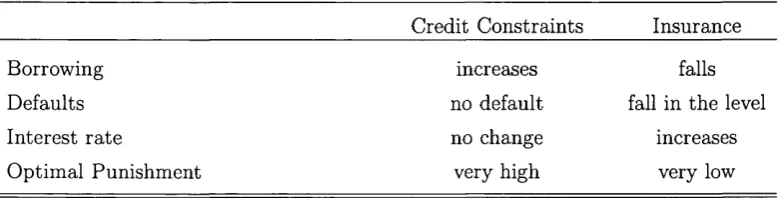
Table 3.1 shows what happens as the level of exemption increases. Suppose th a t income is
exogenous,^ and bankruptcy provided insurance. As the exemption becomes more generous,
the punishment falls. Since default occurs if ç < — while repayment takes place if
q < A2, then reducing g(-) will reduce the level of default. Further, as long as default is
negatively correlated with income, increasing the level of the exemption will further compress
the distribution of second period outcomes, and will provide more insurance. T hat is, the
consumer will want to hold more debt. Lastly, if the bank’s zero profit condition holds,
a simple application of Leibniz’s rule shows th a t the level of the exemption will raise the
interest rate.
The implications of our example or of the model of Kehoe and Levine (1993) or Kocher
lakota (1996) are different. Ruling out default means th a t reducing the punishment will
reduce the level of debt th a t the consumer will be allowed to hold. It will have no effect
on the default rate, since default is never allowed. Interest rates will not change either, all
consumers will pay the riskless rate r-^. There is no interest rate premium as default never
happens.
Table 3.1: Expected effect of increasing the punishment for default.
Credit Constraints Insurance
Borrowing increases falls
Defaults no default fall in the level
Interest rate no change increases
Optimal Punishment very high very low
In section 4 these ideas about holdings of debt are tested using data. A consumer could
be observed in any period of his life, and, in any given period, it is not known whether the
consumer is credit constrained.
3.3
P erson al B an k ru p tcy in th e U n ited States:
The United States contains some of the most generous bankruptcy regulations for default on
debt in the world. The Federal Bankruptcy Act of 1978 specified individuals could choose to
file for personal bankruptcy under either Chapter 7 or under Chapter 13, in cases which were
not deemed a ’substantial abuse’ of the bankruptcy regulations.^ Chapter 7 was limited to
those with assets of less than $750,000 and the aim of the act was to allow those genuinely
unable to repay their debts the chance to have a fresh start. Under the act, the debtor
had his debts expunged, in return for surrendering all his assets except those deemed by
the court necessary for him to make his fresh start: the federal exemptions are shown in
table 3.2.9 u^^jer Chapter 13, the debtor agreed a repayment schedule for part or all of
the debt: in practise a ceiling to how much was going to be repaid under Chapter 13 was
set by the amount th a t the debtor could be forced to surrender under Chapter 7. Many
courts preferred the debtor to file under chapter 13, but enforced purely nominal repayment
schedules. Around 70% of personal bankruptcy cases resulted in a filing for Chapter 7, with
the remainder under Chapter 13.
Where the value of the property was in excess of the exemption, the asset would be sold
and the amount in excess of the exemption went to satisfy the debt. Cash up to the value of
the exemption is retained by the debtor. In some cases the courts insisted th a t the money
had to be re-invested in an exempt asset within a certain amount of time.
3 .3 .1
S ta te E x em p tio n s:
Since bankruptcy had traditionally been regulated by the individual states, the 1978 act
allowed debtors to choose between the exemption allowed by the state and the exemption
resulting in substantial hardship; and in cases where the debtor had changed jurisdiction in order to take advantage of more generous exemptions in the new regime. However, the meaning of substantial abuse did not extend to the ability to repay out of current income, even in cases where current income was high.
Table 3.2: Federal exemptions for Chapter 7 bankruptcy.
Description Amount
$
Comments
Current exemptions:
1. House 15,000
2. Car 2,400
3. Household Goods 8 , 0 0 0 $400 each item (furnishings, goods,
clothes, appliances, books, animals,
musical instruments) for personal
use only.
4. Jewelry 1 , 0 0 0 personal use only.
5. Other Property 800 + $7,500 of (1) th a t is unused.
6. Tools of Trade 1,500 Items needed for job.
Prior to 1994-'
1. House 7,500
2. Car 1 , 2 0 0
3. Household Goods 4,000 $ 2 0 0 each item.
4. Jewelry 500
5. Other Property 400 + $3.750 of (1) th a t is unused.
6. Tools of Trade 750
Prior to 1984:
3. Household Goods no limit on aggregate amount th at
can be claimed under this category.
5. Other Property Allowed all of unclaimed exemption
from (1).
Source: Title, 11, Section 522(d) of the annotated federal code. While not recorded, the federal legislation
set by the federal g o v e r n m e n t I t also allowed each state to refuse to allow the federal
exemptions: the states that have enacted such legislation has been given in table 3.3 below.
In the survey used in this chapter, roughly 18% of people are better off claiming the federal
exemption rather than the state exemption.
Naturally, in cases where he had the option, the debtor would choose the larger of the
state and the federal exemption. The chapter will exploit the differences in the level of the
exemption to assess how the punishment in bankruptcy affects the level of debt and the
amount of consumption smoothing. This chapter is able to exploit changes in the level in
two dimensions; differences across the different states at a point in time, and changes over
time.
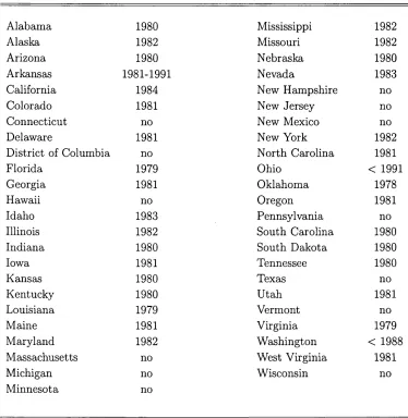
Table 3.3 shows which states have opted out of the federally set bankruptcy exemptions.
As the table shows, most states have disallowed the federal exemptions, and in most cases
where the state has not opted out, the state has enacted its own exemptions which may
be chosen instead of the federal exemption: in these cases the state exemptions are usually
more generous than the exemptions contained in the federal legislation.^^
As for the federal exemptions, each state has set a variety of things th a t are exempt from
seizure or forced sale for the satisfaction of a debt. The federal law demanded th at the state
exemptions should act in the same way as the federal exemptions, except in regard to what
was exempt, and to what value. In many cases the courts have chosen to interpret legislation
in slightly different ways. For example, all states have allowed tools and equipment needed
for work to be exempted, up to a limit. However, some jurisdictions have chosen to allow
^°The source for all the legislation, and legal comments, is derived from the Annotated State Codes published by Westlaw.
Since residents of Montana, North Dakota, Rhode Island, and Wyoming are not sampled in the CEX survey, these states have been excluded from the analysis below.
a car used to drive to work to fall under this definition, while other jurisdictions have not
allowed this. The courts have also allowed debtors substantial room for manoeuvre in fully
exploiting all the exemptions available: in most cases they have allowed the debtor to re
arrange his portfolio of assets prior to default and substitute exempt assets for non-exempt
assets (some limit is placed on the ability to re-arrange assets by ‘abuse/fraud’ provisions).
Since there is considerable scope for substituting between assets when filing for bankruptcy,
the exemptions have been added together, to arrive at a total money value of the exemption
for each state. This chapter has summed the exemption on the homestead to the exemp
tion on other assets but it has excluded the exemption on ’tools of trad e’. The ‘tools of
trad e’ exemption has been excluded since, for the most part, they do not give rise directly to
consumption and thus directly enter the utility function. In any case, including these items
does not substantively change any of the results. As already stated the calculated exemption
value differs between states and across time. It can also differ across subgroups of the popu
lation within the state: many states increase the value of exemptions for older, disabled, or
married people, or if the debtor has other dependents. In cases where the federal exemption
is allowed, the state and federal exemption has been compared and the household has been
assigned the larger of the two e x e m p t i o n s . I n each case it is the overall household’s exemp
tion th a t has been calculated rather than the individuals in the household. This household
exemption will depend on the marital status and age of the household head, on the number
of dependents (both children and old people) and on whether the household head, or his
spouse, is disabled. The exemption will also depend on the date at which the household is
observed, since the exemptions evolve over time.
In calculating the level of exemptions a number of simplifications had to be made. The
homestead exemption is th a t stated in the state legislation. In cases where the homestead
exemption was unlimited^'^, then a dummy was included in the regressions and the value of
California, the household was assigned the larger of the two state exemptions.
Table 3.3: Whether, and in which year, the state passed legislation to not allow the federal
exemptions to be claimed.
Alabama 1980 Mississippi 1982
Alaska 1982 Missouri 1982
Arizona 1980 Nebraska 1980
Arkansas 1981-1991 Nevada 1983
California 1984 New Hampshire no
Colorado 1981 New Jersey no
Connecticut no New Mexico no
Delaware 1981 New York 1982
District of Columbia no North Carolina 1981
Florida 1979 Ohio < 1991
Ceorgia 1981 Oklahoma 1978
Hawaii no Oregon 1981
Idaho 1983 Pennsylvania no
Illinois 1982 South Carolina 1980
Indiana 1980 South Dakota 1980
Iowa 1981 Tennessee 1980
Kansas 1980 Texas no
Kentucky 1980 Utah 1981
Louisiana 1979 Vermont no
Maine 1981 Virginia 1979
Maryland 1982 Washington < 198 8
Massachusetts no West Virginia 1981
Michigan no Wisconsin no
Minnesota no
the continuous exemption was set at the value of the exemption on other items. In cases
where no specific monetary limit was put on a particularly category of goods (for instance
some states had an allowance for “all necessary wearing apparel”) a value was assigned to
the exemption of the good. The following values were adopted: clothes are assigned a value
of $1000, books $1000, pictures $1000, other personal possessions $500, jewellery (including
watches and wedding rings) $1500, home furnishings $5000, and fuel and provisions $500.
The final issue is to consider what happens when either the state or the federal exemption
changes, due to local or national legislation. Most states changed the level of exemptions at
least once (if preferred to the federal exemption), and the federal exemptions also changed in
this period. While most states only made one or two changes during the period, Minnesota
changed the exemption a remarkable seven t i m e s . I n cases where the month in which the
legislation was passed is known (to me), then any observation th at is within three months of
this legislation has been removed. In cases where the month in which the legislation is not
known (the year always is) then all observations for th a t year have been removed.
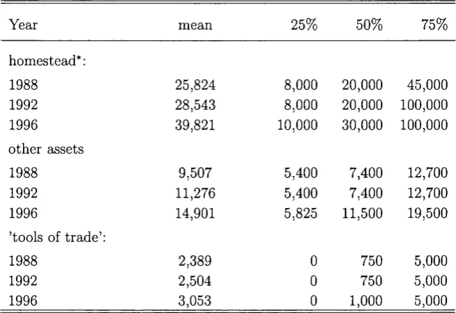
Table 3.4 shows the level of exemptions and how they evolve over time. In most states,
the exemptions rarely change (observe th at the quartiles do not change much) but in most
years at least one state changes its level of exemptions (notice how the means change). The
homestead exemption is typically much larger than the total exemptions for other property
(excluding the ’tools of trad e’ exemption) and this in turn is usually larger than the ’tools
could be claimed.
Arizona, Colorado, Connecticut, Washington DC, Florida, Hawaii, Illinois, Iowa, Maine, Michigan, Missippi, New Jersey, New Mexico, North Carolina, Oklahoma, Oregon, Pennsylvania, South Carolina, South Dakota, Tennessee, Texas, Utah, and Virginia had one change; Alaska, Arkansas, Idaho, Nevada, and Vermont had two changes, California, New Hampshire, and Washington had three changes, Minnesota had seven changes, while Alaska, Georgia, Indiana, Kansas, Kentucky, Louisiana, Maryland, Massachusetts, Missouri, New York and Wisconsin did not change.
of trad e’ exemption. The level of the exemption is growing over time, and there is evidence
of the distribution being skewed to the left, as the mean is larger than the median in all the
cases shown above.
Table 3.4: The level of exemptions (in dollars) over the sample period.
Year mean 25% 50% 75%
homestead* :
1988 25,824 8 , 0 0 0 2 0 , 0 0 0 45,000
1992 28^43 8 , 0 0 0 2 0 , 0 0 0 1 0 0 , 0 0 0
1996 39,821 1 0 , 0 0 0 30,000 1 0 0 , 0 0 0
other assets
1988 9,507 5,400 7,400 12,700
1992 11,276 5,400 7,400 12,700
1996 14,901 5,825 11,500 19,500
’tools of trade’:
1988 2,389 0 750 5,000
1992 2,504 0 750 5,000
1996 3,053 0 1 , 0 0 0 5,000
* In calculating the mean for the homestead exemptions, the unlimited homestead exemptions have been om it
ted.
As an example of how much the legislation can differ, it is instructive to compare the most,
and one of the least generous jurisdictions. In West Virginia a bankrupt has a homestead
exemption of up to $5,000 and can also keep up to $1,000 of other personal property. In
contrasts Texas, the most generous state, allows the home to be exempt from seizure, no
m atter what the value of the house, as well as allowing individuals to keep $15,000 of other
assets (which could include two cars) while other types of households could keep $30,000. In
Both table 3.4 and the comparison between Texas and West Virginia show th at there is
considerable heterogeneity among states with regard to the level of exemptions that may be
claimed as exempt in bankruptcy. It is precisely this heterogeneity th a t will be exploited
in this chapter. States also differ in rules concerning garnishment: court orders th a t take a
proportion of wage income directly from employers to lenders. However, since bankruptcy
overrides garnishment, filing for bankruptcy tends to be higher in states which allow gar
nishment, but may not reflect differences in default (less than a quarter of defaults result
in a flling for bankruptcy). Usury limits also differ across states, but by 1988 these rules
had mostly been repealed. Other possible differences are differences in stigma and in wel
fare rules. A clear assumption is th a t omitted state heterogeneity is orthogonal to the state
bankruptcy exemptions.
3.4
D a ta D escription:
This work uses the Consumer Expenditure Survey, which is described earlier. The chapter
also constructs the total unsecured debts held by the household, including debts held in
revolving credit accounts (including store, gasoline, and general purpose credit cards), in
installment credit accounts, credit at banks or savings and loan companies, in credit unions,
at finance companies, unpaid medical bills, and other credit sources. It also includes negative
balances held in checking or brokerage accounts. Excluded from the total are mortgage,
and other secured debts. This contrasts with the approach taken by Gropp et. al. (1997).
Hynes and Berkowitz (1998) argue th at the impact of bankruptcy exemptions on secured and
unsecured debt ought to be very different, and in their study they consider mortgage debt.
While mortgage (and other secured) debt is also likely to be im portant for the household,
the creditor has an additional claim to such assets in the event of bankruptcy and can
always claim the house (or other security) if the debtor defaults. The housing, or other
exemption will not affect the creditors rights in this case, and hence it does not make sense
to include such debts in the analysis. Other secured debts (for instance on cars) have also
been excluded.
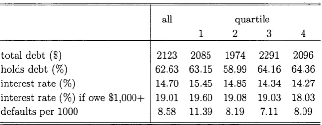
Table 3.5: Summary statistics for different exemption quartiles.
all
1
quartile
2 3 4
total debt ($) 2123 2085 1974 2291 2096
holds debt (%) 62.63 63.15 5&99 64.16 64.36
interest rate (%) 14.70 15.45 14.85 14.34 14.27
interest rate (%) if owe $1,0 0 0+ 19.01 19.60 19.08 19.03 18.03
defaults per 1 0 0 0 8.58 11.39 8.19 7.11 8.09
Table 3.5 gives a brief summary of the data, and compares the different exemption
quartiles of the state exemptions. It shows th at the level of debt changes from quartile
1 (in which the lowest level of assets may be kept) to quartile 4. The average level of debt
held is around $2,100 (the median is $385, while the 75th percentile is $2,250) but there is
no strong pattern to the level of debt. It is also difficult to see a pattern to the number of
people holding at least some debt in the sample. In all cases around 60% of people hold debt.
However, looking at the interest rate suggests laxer rules imply a higher interest rate. The
interest rate is constructed as the reported costs divided by the reported level of debt. The
interest rate is thus the average interest rate on all debts rather than the marginal interest
rate, which is what motivates the marginal borrowing decision. This pattern of interest rates
These results are significant in themselves (at the 10% level) if a one-sided rank-order test
is done. The rate of default, calculated from aggregate d ata as the ratio of the number of
bankruptcy filings, divided by the number of households (rather than individuals) resident in
the state, is much higher for the first quartile for which the highest exemptions, but otherwise
there does not seem to be a clear pattern to the defaults. As might be expected, the pattern
for defaults and the interest rate is similar, but does not match completely: perhaps because
the interest rate not only reflects the probability of default, but also the cost to the lender
of default.
3.5
R egressions:
According to the theory outlined above, debtors will hold debt up to some maximum amount.
By comparing the level of debt th at individuals hold across states, the impact of the state
exemptions can be assessed. Since debts are bounded at zero, a simple tobit model, in
which the level of debt is regressed on a set of household characteristics, and the bankruptcy
exemption to which the household is eligible, can be used. The key assumptions here are th at
household characteristics, and the size of the exemption, are exogenous. Further assumptions
are th at the household’s state of residence is also exogenous, and th a t any changes in the level
of exemptions over time are unexpected. In reality, household’s decisions about education,
residence and fertility may well be related to the ability to smooth consumption: at some
level all economic decisions are endogenous. However, for this discussion it is assumed that
these issues are of secondary importance, and they shall be ignored.
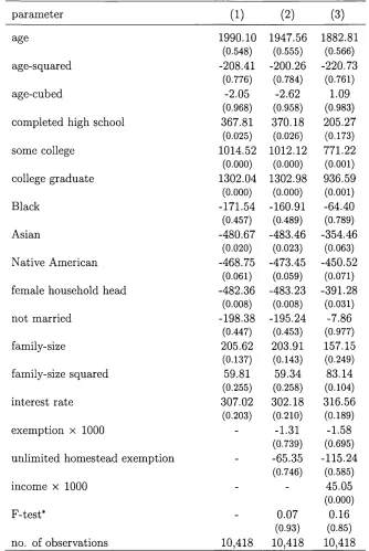
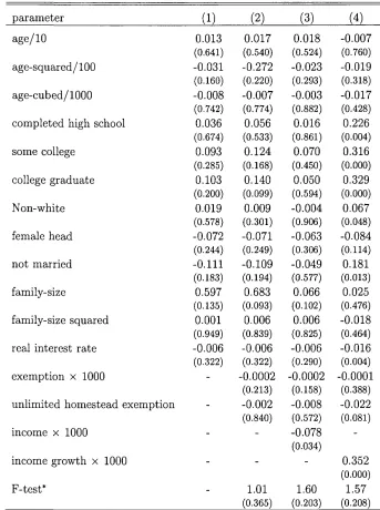
3 .5 .1 R e su lts:
In table 3.6 the results of the tobit are displayed. They show th a t increasing the exemptions
of debt, and the level of income: recall th at example 1 implied th a t there should be a
linear relationship. The first regression shows the coefficients on all the control variables,
without including the exemption variables or income. These variables will partly account for
preferences, and partly account for income. The regression includes age and cohort effects,
which means th at time is excluded (age, cohort and time are collinear). This implicitly
assumes all changes over time in the population is due to individual cohorts aging, and new
cohorts replacing old cohorts, ff year effects are important, then this will show up in the age
and cohort coefficients. However, the paper does not attem pt to interpret these coefficients.
The interest rate th at is included is the municipal bond rate deflated by the inflation rate.
The regression has 10,418 observations: the small number is due to the fact th at only the
second interview for those households with full state information are included. Furthermore,
households who are very close to a change in their exemption level are also excluded (within
three months if the month is known and in the same year if it is not). The reason for
excluding these households, is it is not clear whether one should use the existing exemption,
or the exemption th at may rationally anticipated shortly in the future.
When the level of the exemption is included, (and also dummy for unlimited homestead
exemption,) we find th a t the coefficients are not significant level. A joint test of the level and
including a dummy for the unlimited homestead exemption is also not significant. Although
the negative coefficient is consistent with the simple theory of credit constraints expounded
earlier. Other things to note are th a t households headed by females or non-white people
seem to hold lower levels of debt (which may partly reflect the greater chance they have
of being turned down, see Hajivassiliou and foannides, 2002c). Better educated people also
hold higher levels of debt as well.
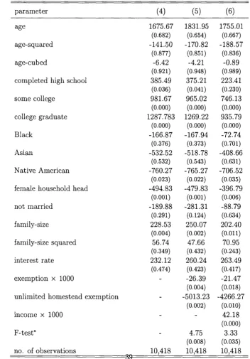
Table 3.7 shows the effect of including state specific dummies, including these state
specific effects ought to control for other state specific effects th a t are not included in the
included, the control variables do not change substantially. However, the effect on the
exemption coefficient is substantial; the results are now highly significant, as shown by the
F-test. This time increasing the level of the exemption from the 25th centile to the 75th
centile entails a reduction in about $1,500. This is large figure, but not implausible, recall
table 3.5 showed the average level of debt is around $2,100 d o l l a r s . T h e true effect is likely
to be under-estimated. The correct regression to run is a tobit which is truncated at zero and
at the point where the credit constraints bite, which, however, is unknown. Unfortunately,
it is not even known if the consumer is credit constrained. The level of debt th at the
consumer will hold will only change for the higher level of exemptions, if the consumer is
credit constrained, and he is able to borrow more money at the lower level of exemptions
(where the punishment for default is bigger). For households th a t are not credit-constrained,
there will be no change in the level of debt th at they hold. Thus the amount calculated from
the table will under-estimate the true effect. It would have been nice to have included time
dummies, to exploit purely the cross-sectional variance, but this is not possible since the
regression already includes age and cohort effects. Clearly age, cohort, and time effects are
not all separately identifiable.^^
A second feature of table 3.7 is that including income in the regression does not substan-
^^The distribution of observed debt may have fatter tails than would be implied by the normality assump tion used in the tobit regression, which may affect the results. A second potentially serious econometric problem is the presence of at least one regressor that contains substantial measurement error. This is an endemic problem with no fully satisfactory solution, consequently all that this paper can do is acknowledge the problem.
tially change the results. Included in the regression is the current level of income. This will
include both temporary and permanent components. If the tem porary component is high
then this will reduce the level of borrowing in the current period, while if the permanent
component is high, then the effects would be a little more ambiguous. Suppose individual
z’s income, denoted y, follows the following process:
Vit — (3.10)
where 2 is a set of other explanatory factors (that evolve over the lifetime), Vi can be
thought of as permanent income, and Su is temporary income. The permanent effect will
unambiguously raise consumption, and it will raise debt in periods where dxa is unusually
low. This is indeed what the regressions find: increasing income does raise the level of debt
that the individual holds.
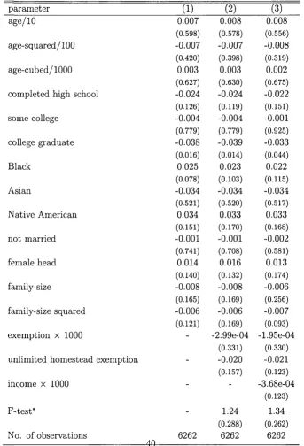
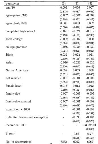
The effect of the exemptions on the interest rate th a t is charged is reported in tables
3.8 and 3.9. The interest rate is the self reported interest rate from the 5th interview and
it is only calculated for those who hold at least some debt. This explains why the sample
size is much smaller than in the other regression. Again, the identifying assumption is th at
the interest rate charged is independent (in a statistical sense) of whether any debt will be
held: we are not just selecting the low interest rate people. This may not be a particularly
appealing assumption in this case. The results suggest th at perhaps better educated people
face lower interest rates, although the effects are small. In table 3.9 neither the level of the
exemptions nor the level of income enter significantly into the results. This is disappointing
given table 3.5, where there is a clear monotonie relationship between the interest rate and
the exemption quartiles. These results could be due to the small sample size and the fact
that self reported interest rates are likely to be measured extremely inaccurately. However,
while this can explain the insignificance of the results in table 3.8 it can not explain the
sign (measurement error in the left-hand side does not bias the point estimates). Table 3.9
significant. The identifying assumption may also be causing these results. As the interest
rate increases, some households would decide not to hold debt, thus downward biasing the
results if the sample is restricted to those holding any debt.^°
3 .5 .2
C o n su m p tio n :
So far these equations have been couched in terms of the level of debt th a t is held by the
household. It is also interesting to think more directly about consumption. For instance,
consider the standard Euler equation for consumption growth th a t has been estimated in
the literature:^^
A l n c i t ^ {r - 5) + (3Xit + U it (3.11)
This framework implies an iso-elastic utility function with relative risk aversion parameter
7 , 5 is the discount rate, while X u represents observed taste shifters, such as family size.
According to the theory, nothing else should enter the regression. However, the literature
has consistently rejected this: current and future income both seem to enter significantly.^^
Two of the most popular explanations for this can be interpreted as having implications for
the error term Uu. Writing
T
Uit = - v a r [cit) + (l)ln (1 - f ipt-i) + £it
then if the relative risk aversion parameter 7 is non-zero, there is a precautionary motive to
saving, and the variance of permanent income Cit will enter the equation. Alternatively, if
some consumers are credit-constrained, the kuhn-tucker condition has an associated multi
plier 'ip, which will be positive when credit constraints are binding. The rejection of equation
Charles (2000) also reports results for a probit on whether any debt is held and on the probability of default, although only the first of these was significant.
^^See, for instance, Deaton (1992)