Opening the black box: interpretable machine learning for geneticists
12
Christina B. Azodi1,2,3¶, Jiliang Tang4, Shin-Han Shiu1,2,5¶ 3
4
1 Department of Plant Biology, Michigan State University, East Lansing, MI, USA 5
2 The DOE Great Lakes Bioenergy Research Center, Michigan State University, East Lansing, 6
MI, USA
7
3 Bioinformatics and Cellular Genomics, St. Vincent’s Institute of Medical Research, Fitzroy, 8
Victoria, Australia
9
4 Department of Computer Science and Engineering, Michigan State University, East Lansing, 10
MI, USA
11
5 Department of Computational Mathematics, Science, and Engineering, Michigan State 12
University, East Lansing, MI, USA
13 14
Corresponding authors:
15
Christina B. Azodi
16
St. Vincent’s Institute of Medical Research
17
9 Princes Street
18
Fitzroy, Victoria, 3065, Australia
19
Tel: +61 04 3396 7476
20
E-mail: [email protected]
21 22
Shin-Han Shiu
23
Michigan State University
24
Plant Biology Laboratories
25
612 Wilson Road, Room 166
26
East Lansing, MI 48824-1312, USA
27
Tel: +1-517-353-7196
28
E-mail: [email protected]
29 30
Key words: interpretable machine learning, deep learning, predictive biology
Abstract
32Machine learning (ML) has emerged as a critical tool for making sense of the growing amount of
33
genetic and genomic data available because of its ability to find complex patterns in high
34
dimensional and heterogeneous data. While the complexity of ML models is what makes them
35
powerful, it also makes them difficult to interpret. Fortunately, recent efforts to develop
36
approaches that make the inner workings of ML models understandable to humans have
37
improved our ability to make novel biological insights using ML. Here we discuss the
38
importance of interpretable ML, different strategies for interpreting ML models, and examples of
39
how these strategies have been applied. Finally, we identify challenges and promising future
40
directions for interpretable ML in genetics and genomics.
41 42
Highlights
43 Machine learning (ML) has emerged as a powerful tool for harnessing big biological
44
data.
45
The complex structure underlying ML models means that their inner logic is not readily
46
intelligible to a human, hence the common critique of ML models as black boxes.
47
However, advances in the field of interpretable ML have made it possible to identify
48
important patterns and features underlying a ML model using various strategies.
49
These interpretation strategies have been successfully applied by researchers in genetics
50
and genomics to derive novel biological insights from ML models.
51
This area of research is becoming increasingly important as more complex and difficult
52
to interpret ML approaches (i.e. deep learning) are being adopted by biologists.
Glossary
55Algorithm: The procedure taken to solve a problem/build a model.
56
Decision tree: A model made up of a series of branching true/false questions.
57
Deep Learning: A subset of ML algorithms inspired by the structure of the brain that can find
58
complex, nonlinear patterns in data.
59
Feature: An explanatory (i.e. independent) variable during modeling.
60
Global interpretation: A ML interpretation that explains the overall relationship between the
61
features and the label for all instances.
62
Instance: A single example from which the model will learn or be applied to.
63
Interpretable: Capable of being understood by a human.
64
Label: The variable to be predicted (i.e. the dependent variable).
65
Local interpretation: A ML interpretation that explains the relationship between the features
66
and the label for one or a subset of instances.
67
Machine learning: Computational models that learn from data without being explicitly
68
programmed.
69
Model: The set of patterns learned for a specific problem, where given input (i.e. instances and
70
their features) the model will generate an output (i.e. prediction).
71
Model performance: A quantitative evaluation of the model’s ability to correctly predict labels.
72
Parameters: Variables in an ML model whose values are estimated/optimized during training.
73
Perturbing strategies: A family of interpretation strategies that measure how changes in the
74
input data impact model predictions or performance.
75
Probing strategies: A family of interpretation strategies that involve inspecting the structure and
76
parameters in a trained model.
77
Surrogate strategies: A family of interpretation strategies that involve training an inherently
78
interpretable model (e.g. a linear model) using the same data as a black-box model to serve as the
79
black-box model's surrogate.
80
Training: The process of identifying the best parameters to make up a model – the learning part
81
in ML.
Importance of interpretable machine learning
83Biological Big Data [1,2] has drivenprogresses in fields ranging from population genetics [3] to
84
precision medicine [4]. Much of this progress is possible because of advances in machine
85
learning (see Glossary; ML; Box 1) [5–10], “[a] field of study that gives computers the ability to
86
learn without being explicitly programmed” [11]. ML works by identifying patterns in data in the
87
form of a model that can be used to make predictions about new data. While powerful, ML also
88
presents new challenges. For example, a common criticism is that the ML models are “black
89
boxes”, meaning their internal logic cannot be easily understood by a human [12]. Luckily,
90
strategies to demystify the inner working of ML models are available and ever improving.
91
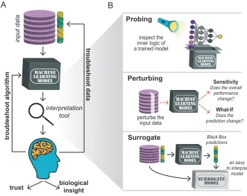
There are three major reasons – troubleshooting, novel insights, and trust – why
92
interpretable ML model, or the ability to understand what logic is driving a model’s prediction,
93
is important (Figure 1A, Key Figure). First, ML models rarely perform well without tweaking or
94
troubleshooting. Understanding how predictions are made is essential for identifying mistakes or
95
biases in the input data and issues with how the model is trained. Second, an ML model with
96
impressive performance may have identified biologically novel patterns. However, such insights
97
will only be available if the model can be interpreted. Finally, we are unlikely to trust a
98
prediction if we do not understand why it was made. For example, a doctor may not trust a ML
99
diagnosis with no supporting justification out of concern that the model may be capturing
100
artifacts or have unknown biases or limitations [13].
101
Overview of strategies for interpretable machine learning
102A wide range of strategies for interpretable ML have been developed and applied to problems in
103
genetics and genomics [14–16]. These strategies can be characterized based on if they are
104
applicable to all ML algorithms (i.e. model-agnostic) or only to one or a subset of algorithms
105
(i.e. model-specific). They can also be characterized based on if they provide global or local
106
interpretations. Global interpretations involve explaining the overall relationship between
107
features and labels. While local interpretations focus on explaining the prediction of an
108
individual instance. For example, imagine you train an ML model to predict if a gene (an
109
instance) is up-regulated after some treatment (the label) based on the presence or absence of a
110
set of regulatory sequences (the features). A global interpretation strategy will tell you how
important regulatory sequence X is for predicting up-regulation across all genes in your dataset.
112
While a local interpretation strategy will tell you how important regulatory sequence X is for
113
predicting gene Y as up-regulated. This means that the type of interpretation strategy you select
114
will dictate what you will learn from your ML model, with different strategies possibly telling
115
different stories. We should also emphasize that ML models identify association through
116
correlation, thus ML interpretation strategies do not identify causal relationships between input
117
features and labels. Instead, interpretations should be used to generate new hypotheses that can
118
be tested experimentally. We will review three general ML interpretation strategies: probing,
119
perturbing, and surrogate strategies (Figure 1B; [14,16]).
120
Probing strategies dissect the inner structure of ML models
121Training an ML model involves identifying the set of parameters best able to predict the label
122
of an instance (e.g. gene Y is up-regulated). After training, these parameters can be probed (or
123
inspected) to better understand what the model learned. Probing strategies provide global
124
interpretations with some exceptions (e.g. DeepLIFT, see below). Because type of parameters
125
and structure of how they connect to each other varies by algorithm, probing strategies are
126
model-specific. While probing strategies are straightforward for some ML algorithms (e.g.
127
Support Vector Machine; SVM; and decision tree-based algorithms), this is not the case for
128
more complex ML algorithms (e.g. deep learning).
129
Probing Support Vector Machine models
130
SVM is an algorithm that finds the hyperplane that best separates instances by their label
131
when they are plotted in n-dimensional space (n = number of features). Training an SVM model
132
to predict gene up-regulation using regulatory sequences as features means learning the
133
combination of weights to apply to each regulatory sequence (i.e. coefficient weight) in order to
134
make the best hyperplane (Figure 2A). SVM models can be trained to learn either linear or
non-135
linear relationships between features and labels. While there are advanced methods for probing
136
non-linear SVM models [17,18], in most biological applications of SVM, only linear SVM
137
models are probed.
138
A trained linear SVM model is probed by extracting the coefficient weights that define
139
the hyperplane (Figure 2A), where features assigned a higher absolute weight have a stronger
140
relationship with the label and thus are more important for driving the prediction. For example, a
linear SVM model was trained to classify simulated populations as being under positive or
142
negative selection using genetic markers as features [19]. Genetic markers with large, positive
143
coefficient weights in the SVM model were the same as those associated with positive selection
144
using classical population genetics statistical tests (e.g. Tajima’s D).
145
Importantly, SVM probing strategies (like other strategies discussed below), can provide
146
an incomplete picture of feature importance. For example, two highly correlated features will
147
split the weight between them, reducing their perceived importance. Or a feature with a strong
148
non-linear relationship with the label may not be assigned a large weight by a linear SVM model
149
and will therefore be missed when the trained model is probed.
150
Probing decision tree-based models
151
A decision tree is a set of true/false questions nested in a hierarchical structure. They are
152
inherently interpretable because the content and order of each question can be directly observed.
153
How well a true/false question separates instances by their label can also be quantified using
154
metrics such as the mean decrease in node impurity. In Figure 2B,using the presence/absence of
155
regulatory sequence “AACGT” to separate up- from down-regulated genes results in a decrease
156
in the mean node impurity. Because single decision trees tend to perform poorly at predicting
157
complex patterns, ensemble approaches (e.g. Random Forest, Gradient Tree Boosting [20]),
158
where many decision trees are combined to generate one prediction, are often used. Ensemble
159
decision-tree models can be probed by calculating the mean decrease in node impurity for each
160
feature across all trees in the ensemble. This approach was used determine which DNA motifs
161
were the most important for predicting if a gene would be differentially expressed under salt
162
stress conditions in Arabidopsis thaliana [21].
163
The hierarchical structure of decision tree-based models means that interactions between
164
features an be readily probed. For example, using a tool for finding stable feature interactions in
165
Random Forest models [21], Vervier and Michaelson identified interactions between genomic,
166
transcriptomic, and epigenomic features that were predictive of deleterious genetic variants [23].
167
Specifically, that an interaction between the local GC content and the distance to the nearest
168
expression Quantitative Trait Loci was important for predicting deleterious variants.
169
As with coefficient weights from SVM models, mean decrease impurity scores can be
170
misleading when features are highly correlated. This score also tends to inflate continuous over
171
categorical features, categorical features with a larger number of categories, and continuous
features with a larger numeric range and should therefore be interpreted with caution when
173
feature space is not uniform [24].
174
Probing deep learning networks
175
While the classical ML algorithms described above are readily interpretable, deep
176
learning(Box 2) algorithms are being applied more and more in the ML community because
177
they frequently outperform classical ML algorithms at modeling complex systems [25–27] and
178
they can learn from raw data (e.g. whole DNA sequence) rather than user defined features (e.g.
179
known regulatory sequences). However, there is often a tradeoff between predictability and
180
interpretability [28], and this is certainly the case for deep learning [29]. Fortunately, there has
181
been a substantial effort to develop new methods to interpret these complex models. First we
182
describe three general approaches to calculate feature importance scores by probing deep
183
learning models: connection weights-based, gradient-based, and activation level-based
184
approaches (Figure 2C) [15].
185
Connection weight-based feature importance scores quantify the global relationship
186
between each feature and the output by summing the learned weights assigned to connections
187
between nodes in input-to-hidden, one or more hidden-to-hidden, and hidden-to-output layers for
188
each input feature [30,31]. Following the path through the example artificial neural network
189
(Figure 2C), the connection weights (represented by line widths) between some features (e.g. f1) 190
and the output layer are larger than the connection weights between other features (e.g. f3) and 191
the output layer, indicating f1 is more important for that model. This approach was used to 192
determine which microRNA features were the most important for predicting the expression level
193
of Smad7, a gene involved in disrupting a signaling process up-regulated in patients with breast
194
cancer [32]. Connection weight-based feature importance scores can be misleading when feature
195
are on different scales, when positive and negative connection weights cancel each other out, or
196
when a connection has a large weight but is rarely activated (i.e. the nodes is rarely turned on)
197
[33].
198
The gradient-based feature importance scores (a.k.a. Saliency) also quantify the global
199
relationship between a feature and the output, but do so by calculating the gradient, or the change
200
in the predicted output (e.g. the likelihood a gene is up-regulated) as small changes are made to
201
the input feature (e.g. the frequency of regulatory sequence X). The gradient is calculated using a
202
handy calculus trick, the partial derivative [34]. This approach was used to identify putative
distal regulatory sequences in genomic regions where positive and negative gradient-based
204
importance score peaks represented enhancer and silencer regions, respectively [35]. This
205
approach is not useful when input features are categorical or when small changes in the feature
206
value do not change the output prediction [33].
207
Finally, the activation level refers to the output value from a node after it has passed
208
through a non-linear function (i.e. the activation function; see Box 2). Activation level-based
209
feature importance scores provide a local interpretation for an instance of interest by comparing
210
how much each feature activates nodes in the trained network compared to the feature values
211
from a reference instance. A reference instance for an image classification model could be one
212
that is solid white, while a reference for a model using a DNA sequence as instances could be an
213
instance with the background nucleotide frequency at every site. This approach (coined
214
DeepLIFT [33]), has been used in multiple biological studies [36–38]. For example, Zuallaert et 215
al. used DeepLIFT to find nucleotide sequences important for predicting splice sites [37].
216
Because DeepLIFT probes activation levels rather than connection weights, it avoids the pitfall
217
of the connection weight-based approach. Further, because it compares a specific instance to a
218
reference, it also avoids the pitfalls of the gradient-based approach.
219
Another way to probe deep learning models is to learn what pattern each node in the
220
network learned to identify (Figure 2C). This can be done by finding real or simulated instances
221
that maximally activate that node, then the properties of those real or simulated instances can be
222
used to interpret that node. For example, if the 10 DNA sequences that maximally activate node
223
X (i.e. cause node X to have the maximum possible output value after passing through the
224
activation function) all contain the motif ACGGTC, one could infer that node trained to find the
225
ACGGTC motif. Because probing every node in every layer may produce results that are still too
226
complex to interpret, dimensionality reduction techniques can be used to ease interpretation. For
227
example, Esteva et al. used a dimensionality reduction technique to visualize the nodes in the last
228
hidden layer of a convolutional neural network (see Box 2) trained to diagnose different types of
229
skin cancer from photos [39]. This allowed them to visualize how well their convolutional neural
230
network learned to separate different types of carcinomas.
Perturbing strategies for interpreting machine learning models
232Perturbing strategies involve modifying the input data and observing some change in the model
233
output. Because modifications to the input data can be made regardless of the ML algorithm
234
used, perturbing strategies are generally model-agnostic. We discuss two general
perturbation-235
based strategies: sensitivity analysis and what-if methods (Figure 3).
236 237
Sensitivity Analysis
238
Sensitivity analysis involves modifying an input feature and measuring the impact on
239
model performance (Figure 3A). Feature modification typically means removing (i.e.
leave-240
one-feature-out) or permuting (e.g. set all values to the mean) one feature at a time. The decrease
241
in model performance after a feature is removed or permuted is an intuitive score for each feature
242
indicating its contribution to the predictions (Figure 3A). Because perturbing a feature not only
243
impacts that feature but also other features that interact with it, sensitivity analysis also captures
244
interaction effects for each feature. However, sensitivity analysis can miss important features if
245
correlation exists in the feature set. For example, if features X and Y are highly correlated,
246
feature Y could compensate when X is removed or permuted, masking its potential importance.
247
Che et al. used the leave-one-feature-out approach to find that genomic region length was
248
the most important feature for identifying genomic regions that contain clusters of genes
249
acquired by horizontal gene transfer [40]. Leave-one-feature-out analysis is computationally
250
expensive because it requires training a new model for every perturbed dataset. Therefore, it is
251
typically not used to interpret deep learning model (which are already computing intensive)
252
except when there are few input features. For example, leave-one-feature-out was used to
253
determine that, of five histone marks, removing H3K4me3 resulted in the largest decrease in a
254
deep learning model’s ability to predict TF binding sites [41].
255
Permutation strategies determine feature importance score by measuring how the
256
performance of an ML model changes when different features are randomly permuted. They are
257
more computationally efficient than leave-one-feature-out strategies because only one model
258
needs to be trained. This strategy is particularly intriguing for genetic studies because its logic is
259
similar to DNA mutagenesis experiments. It was demonstrated that in silico mutagenesis (i.e.
260
computationally permuting DNA sequence) could identify which nucleotides impact tissue
specific gene expression the most [42]. A permutation-based strategy used in image analysis is
262
called occlusion sensitivity. Here different regions in images are grayed out and the resulting
263
change in performance is measured. For example, occlusion of regions of blood smear images
264
confirmed that a malaria classification model performed worst when parasitized regions were
265
grayed out [43].
266 267
What-if Analysis
268
The what-if approach (a.k.a. counterfactuals [44]) measures how the prediction of a
269
particular instance changes (rather than the overall model performance) when the input value for
270
one or more features is changed. Thus, what-if analysis provides local interpretations while
271
sensitivity analysis provides global interpretations. Here we focus on two what-if methods:
272
partial dependency plots (PDPs) and individual conditional expectation (ICE) plots (Figure 3B;
273
[16]).
274
PDPs show how a prediction changes when the input value for a feature of interest is
275
changed, marginalizing (i.e. ignoring) the effects of all other features [45]. Imagine we trained a
276
ML model that predicts the likelihood that a sequence will be bound by a certain transcription
277
factor (TF). A PDP would show, for example, how the TF-binding likelihood would change if
278
the nucleotide at position of interest is changed from C to A, G or T (left panel, Figure 3B). This
279
approach was used to demonstrate the impact of sequence features (e.g. amino acid identity,
280
conservation) on the predicted efficacy of a guide RNA for CRISPR-Cas9 [46]. PDPs can miss
281
important features when there are interactions between features. For example, imagine if a C at
282
position #3 increased TF binding affinity when position #2 contained a T but decreased binding
283
affinity if position #2 contained an A. Because position #2 is marginalized in the position #3’s
284
PDP, the interaction may mask the importance of position #3.
285
ICE plots were proposed to address this limitation of PDPs [47]. ICE plots are essentially
286
PDPs generated for every individual instance in the dataset. For example, an ICE plot for
287
position #3 would show that the presence of a C at position #3 only increases the TF binding
288
likelihood in the subset of sequences, which with further investigation we find are the sequences
289
with a T in position #2 (right panel, Figure 3B). Because this strategy does not require model
re-290
training, it is well suited for interpreting deep learning models. For example, ICE plots were used
291
to better understand what patterns of gene expression an adversarial deep learning model (see
Box 2, Figure IIB) learned were characteristic of single cell data [48]. By varying the expression
293
level of individual genes (the feature) within the single cell (the instance), they found the genes
294
with the biggest impact on the prediction (real or not) were genes known to be markers for
295
particular cell-type states (e.g. IvI, Krt10, and Krt14 for epidermal cell state).
296
What-if analyses can provide highly detailed and intuitive interpretations of ML models,
297
including the magnitude, direction, and non-linearities in the relationships between features and
298
the output label. A limitation is that PDP and ICE plots can only be visualized for one or two
299
features at a time, so they are typically only generated for models with few features or with a
300
subset of features deemed important by another interpretation strategy or from domain
301
knowledge [49].
302
Surrogate strategies for interpreting machine learning models
303Image you have an ML model that is truly a black box—meaning that it cannot be probed and
304
perturbations strategies do not provide useful information. In such a case, one can train an
305
inherently interpretable model (e.g. linear model or a decision tree) to act as a surrogate for the
306
black box model. For example, to generate a surrogate model for a black box model that can
307
predict gene up-regulation using regulatory elements as features, we would first apply the black
308
box model to a set of genes, G, and extract the black box predicted label (i.e. up- or
down-309
regulated) for those genes (Figure 1B). Then we would use the same set of genes G as the
310
instances and the black box predicted labels as the labels to train an interpretable surrogate
311
model.
312
One major limitation of surrogate models is that black box models are often highly
313
complex (e.g. highly non-linear, many higher order interactions), and thus, cannot be fully
314
learned by an interpretable surrogate. To overcome this, one approach is to generate a surrogate
315
to learn just a portion of the black box model, known as a Local Interpretable Model-agnostic
316
Explanations (LIME; [50]). While the complex logic underlying the whole model may be too
317
much for a surrogate model to learn, the logic for one instance or a group of similar instances
318
(e.g. co-expressed genes) may be simple enough. For example, LIME was used to better
319
understand why some patients (i.e. instances) were misclassified by a black box model predicting
320
survival after cardiac arrest [51]. A LIME model for a patient that was mis-predicted to survive
321
showed that the black box model was too heavily influenced by certain features (e.g. healthy
neurologic status, lack of chronic respiratory illness) and did not place sufficient weight on other
323
features that are also important (e.g. elevated creatinine, advanced age).
324
Concluding Remarks
325Interpretability is critical for applications of ML in genetics and beyond and will therefore see
326
substantial advances in the coming years. Just as there is no one universally best ML algorithm,
327
there will not likely be one ML interpretation strategy that works best on all data or for all
328
questions. Rather, the interpretation strategy should be tailored to what you want to learn from
329
the ML model and confidence in the interpretation will come when multiple approaches tell the
330
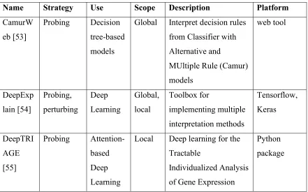
same story. Luckily, many user-friendly tools have already been developed to facilitate
331
interpreting ML models using the strategies described in this review and more (Table 1). The
332
insights that can be learned from interpreting a ML model are constrained by the content, quality,
333
and quantity of the data used to generate the model. Care should be taken when selecting data
334
and features to avoid introducing technical or biological artifacts into the models, and thus into
335
the interpretations.
336
There are still many challenges to interpreting machine learning models in genetics and
337
genomics (see Outstanding Questions). These challenges, while not necessarily unique to
338
genetics or genomics, represent opportunities for computational biologists to innovate and
339
contribute novel solutions. They also highlight the importance of training the next generation of
340
biologists able to work at the intersection of computer and biological science.
341
Acknowledgement
342We thank Yuying Xie for his insightful feedback on this review. This work was partly supported
343
by the National Science Foundation (NSF) Graduate Research Fellowship (Fellow ID:
344
2015196719) to C.B.A.; NSF (IIS-1907704, IIS-1845081, CNS- 1815636) grants to J.T.; and the
345
U.S. Department of Energy Great Lakes Bioenergy Research Center (BER DE-SC0018409) and
346
NSF (IOS-1546617, DEB-1655386) grants to S.-H.S.
Outstanding Questions
348 How can we interpret ML models trained on heterogeneous (e.g. multi-omic) and high
349
dimensional (number of features >> number of instances) data? ML algorithms are well
350
suited to take advantage of the large-scale multi-omic data for generating predictive
351
models. However, interpreting ML models trained on high dimensional and heterogenous
352
data remains challenging. These challenges are exasperated when features are highly
353
correlated and of different types (e.g. continuous verses binary).
354
What ML modeling and interpretation strategies are best for studying complex biological
355
systems? Given the importance of non-linear effects in biology (e.g. epistasis, feedback
356
loops, community dynamics, synergistic/antagonistic effects), interpretation strategies
357
that can identify features that have important but complex effects are critical.
358
How can we compare ML interpretation strategies and results? The strategies used to
359
interpret an ML model are able to identify different aspects of the logic underlying that
360
model. How can we benchmark new and established interpretation strategies for
361
applications in genetics and genomics? Further, how could we join the findings from
362
multiple strategies into a fuller, yet still coherent, interpretation of that model?
363
How can interpretable ML become an accessible tool for biologists? Implementing ML
364
interpretation strategies can require extensive computational knowledge. What roles will
365
interdisciplinary training (e.g. computer science, data science) and the
user-friendly-366
software play in encouraging the interpretation of ML models in genetics and genomics?
367
How can researchers ensure that model interpretability will continue to be an area of
368
development for folks working in the artificial intelligence field? As the power and
369
precision of ML models improves, more and more trust will likely be placed in them.
370
What role can researchers play in shaping the future of AI?
371 372
Text Boxes
373Box 1: A crash course in machine learning.
374
Machine Learning (ML) is when a computer uses data to learn a model for predicting a
375
value, where the relationship between the data and the value is not explicitly provided. The data
is composed of instances (i.e. samples) and feature (i.e. independent variables) that describe
377
those instances. For example, if our instances are genes, features describing those genes could be
378
the GC content, the presence or absence of a specific functional domain, or its level of
379
conservation across species. If the values being predicted are not known a priori for any instance,
380
then unsupervised ML approaches (e.g. clustering) can be applied to extract previously unknown
381
patterns. If the values being predicted are known for some of the instances, these values are
382
referred to as labels and one can learn from these labels and turn the problem into a supervised
383
ML problem. Further, if the known labels are categorical (e.g. is the gene up-regulated or
down-384
regulated), it is a classification problem, while if the labels are continuous (e.g. gene expression
385
levels), it is a regression problem.
386
A common supervised ML workflow involves four steps: training, applying, scoring, and
387
interpretation (Figure I). First, input data made up of features and labels for many instances are
388
divided into a training set and a testing set. The features and labels from the training set are then
389
used to train the ML model. During training, the ML model learns the combination of internal
390
parameters that minimize the error in the predictions of the labels. Second, the trained ML model
391
is applied to the testing set features to generate predicted labels. A trained ML model can also be
392
applied to unlabeled instances to make predictions. Third, the performance of the ML models is
393
scored by comparing the predicted labels with the known labels from the test set. Many different
394
performance metrics are used in the ML field, where the best metric depends on the type of ML
395
problem and the nature of the question being asked. A performance metric not only informs the
396
quality of a model, but also provides a quantitative measure of how much we known about the
397
biological phenomenon in question given the features used. Finally, the ML model is interpreted
398
to provide a better, quantitative understanding on how the input features contribute to the
399
predictions.
400 401
Figure I. A supervised machine learning workflow.
402 403
Box 2: A crash course in deep learning.
404
ML algorithms inspired by the structure of the brain make up a subfield of ML called
405
Deep Learning (DL). DL is promising for biology because DL models can 1) learn highly
406
complex nonlinear patterns, 2) continue to improve when given more training data (“shallow”
ML models tend to plateau), and 3) they can learn from raw data without user defined features
408
[52]. A DL model is made up of multiple layers of nodes connected by edges of different
409
connection weights (wx) (Figure IIA). The nodes in the input layer contain the feature values (fx)
410
for an instance. The nodes in the hidden layers (hidden nodes) represent the sum of the nodes
411
from the previous layer multiplied by their associated connection weights (∑wxfx). The node
412
value from that summation is then passed through an activation function (represented as a light
413
switch), which determines the extent to which that node gets turned on (i.e. activated). A DL
414
models are able to learn nonlinear relationships when the activation function used is nonlinear
415
(e.g. the sigmoid function). The output node (i.e. the predicted label) is the sum of the nodes
416
from the last hidden layer and can be compared to the true label to calculate the error in the
417
model. A DL model is trained by propagating that error back through the model and updating the
418
learned connection weights (i.e. backpropagation of the error) until that error is minimized.
419
While this type of DL algorithm, often referred to as a fully-connected artificial neural
420
network, is useful for modeling complex, nonlinear relationships. Other DL algorithms many be
421
useful for addressing different biological questions (Figure IIB). For example, convolutional
422
neural networks learn spatial patterns making them ideal for identifying sequence motifs and
423
patterns in images, while recurrent neural networks remember earlier predictions and are
424
therefore ideal for sequential data analysis.
425 426
Figure II. Graphical explanations of deep learning algorithms. (A) An example
fully-427
connected artificial neural network. (B) Uses, graphical explanations, and example biological
428
applications for three additional deep learning algorithms: Convolutional Neural Networks,
429
Recurrent Neural Networks, and Adversarial Learning.
430 431
Figure Legends
432Figure 1. Overview of ML model interpretation strategies
433
(A) Understanding the inner logic of a machine learning (ML) model (i.e. model interpretability),
434
is important for troubleshooting during model training, generating biological insights, and
435
instilling trust in the predictions made. (B) There are three general strategies for interpreting a
436
ML model: probing, perturbing, and surrogates. Probing strategies involve inspecting the
structure and parameters learned by a trained ML model (e.g. a deep learning model pictured
438
here) in order to better understand what features or combination of features are important for
439
driving the model’s predictions. Perturbing strategies involve changing values of one or more
440
input features (e.g. setting all values to zero) and measuring the change in model performance
441
(sensitivity analysis) or on the predicted label of a specific instance (what if analysis). Finally, an
442
easily interpretable model (e.g. linear regression or decision tree) can be trained to predict the
443
predictions from a ML models, acting as a surrogate.
444 445
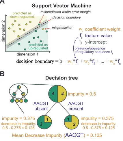
Figure 2.Probing a trained machine learning model.
446
An ML model that classifies up- (green) from down-regulated (yellow) genes using regulatory
447
sequences (purple) as features can be probed to find what regulatory sequences are most
448
important for predicting differential expression. (A) Asupport vector machine model learns the
449
combination of coefficient weights (w; orange) that form the decision boundary (dotted line) best
450
able to separate up- from down-regulated genes, where the features assigned the higher w are
451
more important. The decision boundary is a hyperplane represented by the equation shown. (B)
452
A decision tree-based model learns the most predictive series of true/false questions about the
453
features. Here we zoom in on a node where the regulatory sequence “AACGT” is used as the
454
feature. How well AACGT separates up- from down-regulated genes is quantified by calculating
455
the mean decrease in node impurity after AACGT is used. Large impurity scores (here calculated
456
as the Gini Impurity) mean the node contains a mix of up and down-regulated genes, while an
457
impurity score equal to zero would indicate the node only contains up or down-regulated genes.
458
(C) Deep learning models train to learn what combinations of connection weights (gray lines)
459
across all nodes and layers results in the network best able to classify up- from down-regulated
460
genes. A trained deep learning models can be probed by inspecting the size of the connection
461
weights (gray line thickness), measuring the gradient of the output with respect to the input [i.e.
462
Out(in)/ (in)], and quantifying the extent to which different features cause a node to activate
463
(represented by the light switch).
464 465
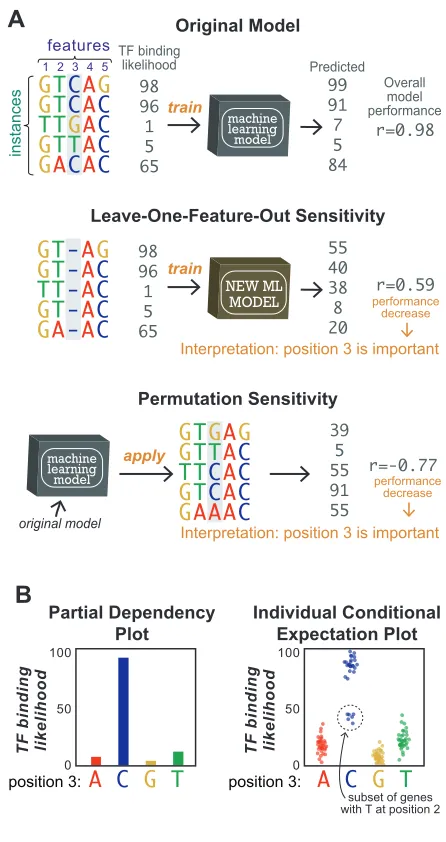
Figure 3. Perturbing the input to a machine learning model.
466
An example ML model predicting if a Transcriptional Factor (TF) may bind (i.e. the label) to a
467
specific sequence (i.e. the features) can be interpreted with perturbing strategies. (A) Sensitivity
analysis. Leave-one-feature-out means a new ML model is trained on the same input data with
469
one feature (e.g. position 3) removed. Then the overall performance of the original model and the
470
new model are compared. Permutation means the original model is applied to input data with the
471
values shuffled for one feature at a time. The performance of the model applied to the original
472
and the shuffled data are compared. Both sensitivity analyses on position 3 shown here resulted
473
in a decrease in performance, leading to the interpretation that position 3 is important for TF
474
binding. (B) What-If analysis. The partial dependency plot (left) shows the TF binding likelihood
475
if position 3 was an A, C, G, or T, ignoring the effects of nucleotides at other positions. This plot
476
shows that a C at position 3 increases the likelihood of TF binding. The individual conditional
477
expectation plot (right) shows the TF binding likelihood score for every instance (dot) in the
478
dataset when position 3 is A, C, G, or T. This plot shows when position 3 is C, the binding
479
likelihoods have a bimodal distribution which is due to interaction with position 2 in this
480
hypothetical example.
481 482
Table Legends
483Table 1. Platforms and software available for interpretable machine learning 484
Name Strategy Use Scope Description Platform
CamurW eb [53]
Probing Decision tree-based models
Global Interpret decision rules from Classifier with Alternative and
MUltiple Rule (Camur) models
web tool
DeepExp lain [54]
Probing, perturbing
Deep Learning
Global, local
Toolbox for
implementing multiple interpretation methods
Tensorflow, Keras
DeepTRI AGE [55]
Probing Attention-based Deep Learning
Local Deep learning for the Tractable
Individualized Analysis of Gene Expression
iml: interpreta ble ML [16] Probing, perturbing Model agnostic Global, Local Toolbox for implementing multiple interpretation methods. R package iNNvesti gate [56]
Probing Deep
Learning Global, Local Toolbox for implementing multiple interpretation methods. Keras
iRF [22] Probing Random
Forest
Global Decision tree based method to identify significant feature interactions.
R package
LIME [50]
Surrogate Model Agnostic
Local A tool to generate local surrogate models for Black-Box models. Python package Lucid (github.c om/tenso rflow/luci d)
Probing Deep Learning
Global, local
Toolbox of methods for visualizing and interpreting neural networks. Tensorflow NeuralNe tTools [57] Probing, perturbing Deep Learning Global, local Toolbox for implementing multiple interpretation methods. R package SpliceRo ver [37]
Probing Deep
Learning
Local Tool to interpret which nucleotides contribute most predicting splice sites using DeepLIFT
web tool The What-If Tool (https://p air-Probing, perturbing Model Agnostic Global, local
Code free toolbox for assessing, comparing, and interpreting Tensorflow/python-based ML models
485
References
4861 Marx, V. (2013) Biology: The big challenges of big data. Nature 498, 255–260 487
2 Stephens, Z.D. et al. (2015) Big Data: Astronomical or Genomical? PLOS Biol. 13, e1002195 488
3 Schrider, D.R. and Kern, A.D. (2018) Supervised Machine Learning for Population Genetics: 489
A New Paradigm. Trends Genet. 34, 301–312 490
4 Alyass, A. et al. (2015) From big data analysis to personalized medicine for all: challenges 491
and opportunities. BMC Med. Genomics 8, 33 492
5 Angermueller, C. et al. (2016) Deep learning for computational biology. Mol. Syst. Biol. 12, 493
878–16 494
6 Chicco, D. (2017) Ten quick tips for machine learning in computational biology. BioData
495
Min. 10, 35 496
7 Cuperlovic-Culf, M. (2018) Machine Learning Methods for Analysis of Metabolic Data and 497
Metabolic Pathway Modeling. Metabolites 8, 4 498
8 Libbrecht, M.W. and Noble, W.S. (2015) Machine learning applications in genetics and 499
genomics. Nat. Publ. Group 16, 321–332 500
9 Ma, C. et al. (2014) Machine learning for Big Data analytics in plants. Trends Plant Sci. 501
10 Tarca, A.L. et al. (2007) Machine Learning and Its Applications to Biology. PLOS Comput.
502
Biol. 3, e116 503
11 Samuel, A.L. (1959) Some Studies in Machine Learning Using the Game of Checkers. IBM J.
504
Res. Dev. 3, 210–229 505
12 Lipton, Z.C. (2018) The Mythos of Model Interpretability. ACM Queue 16, 506
13 Miller, T. (2019) Explanation in artificial intelligence: Insights from the social sciences. Artif.
507
Intell. 267, 1–38 508
14 Guidotti, R. et al. (2018) A Survey of Methods for Explaining Black Box Models. ACM
509
Comput. Surv. 51, 1–42 510
15 Montavon, G. et al. (2018) Methods for interpreting and understanding deep neural 511
networks. Digit. Signal Process. 73, 1–15 512
16 Molnar, C. (2019) Interpretable Machine Learning: A Guide for Making Black Box Models
513
Explainable, 1st edition.Christoph Molnar. 514
17 Barakat, N. and Bradley, A.P. (2010) Rule extraction from support vector machines: A 515
review. Neurocomputing 74, 178–190 516
18 Rasmussen, P.M. et al. (2011) Visualization of nonlinear kernel models in neuroimaging by 517
sensitivity maps. NeuroImage 55, 1120–1131 518
19 Ronen, R. et al. (2013) Learning Natural Selection from the Site Frequency Spectrum. 519
Genetics 195, 181–193 520
20 Breiman, L. (2001) Random Forests. Mach. Learn. 45, 5–32 521
21 Uygun, S. et al. (2019) Cis-regulatory code for predicting plant cell-type transcriptional 522
response to high salinity. Plant Physiol. DOI: 10.1104/pp.19.00653 523
22 Basu, S. et al. (2018) Iterative random forests to discover predictive and stable high-order 524
interactions. Proc. Natl. Acad. Sci. 115, 1943–1948 525
23 Vervier, K. and Michaelson, J.J. (2018) TiSAn: estimating tissue-specific effects of coding and 526
non-coding variants. Bioinformatics 34, 3061–3068 527
24 Strobl, C. et al. (2007) Bias in random forest variable importance measures: Illustrations, 528
sources and a solution. BMC Bioinformatics 8, 529
25 Banerjee, S. et al. (2017) , Performance of Deep Learning Algorithms vs. Shallow Models, in 530
Extreme Conditions - Some Empirical Studies. , in Pattern Recognition and Machine
531
Intelligence, pp. 565–574 532
26 Guo, Y. et al. (2016) Deep learning for visual understanding: A review. Neurocomputing 187, 533
27–48 534
27 LeCun, Y. et al. (2015) Deep learning. Nature 521, 436–444 535
28 Kuhn, M. and Johnson, K. (2013) Applied Predictive Modeling, 536
29 Schmidhuber, J. (2015) Deep learning in neural networks: An overview. Neural Netw. 61, 537
85–117 538
30 Garson, D.G. (1991) Interpreting neural network connection weights. AI Expert 6, 46–51 539
31 Olden, J.D. and Jackson, D.A. (2002) Illuminating the “black box”: a randomization approach 540
for understanding variable contributions in artificial neural networks. Ecol. Model. 154, 541
135–150 542
32 Manzanarez-Ozuna, E. et al. (2018) Model based on GA and DNN for prediction of mRNA-543
Smad7 expression regulated by miRNAs in breast cancer. Theor. Biol. Med. Model. 15, 544
33 Shrikumar, A. et al. (2017) Learning Important Features Through Propagating Activation 545
Differences. Proc. 34 Th Int. Conf. Mach. Learn. at 546
<http://proceedings.mlr.press/v70/shrikumar17a/shrikumar17a.pdf> 547
34 Simonyan, K. et al. (2013) Deep Inside Convolutional Networks: Visualising Image 548
Classification Models and Saliency Maps. Int. Conf. Learn. Represent. at 549
<http://arxiv.org/abs/1312.6034> 550
35 Kelley, D.R. et al. (2018) Sequential regulatory activity prediction across chromosomes with 551
convolutional neural networks. Genome Res. 28, 739–750 552
36 Washburn, J.D. et al. (2019) Evolutionarily informed deep learning methods for predicting 553
relative transcript abundance from DNA sequence. Proc. Natl. Acad. Sci. 116, 5542–5549 554
37 Zuallaert, J. et al. (2018) SpliceRover: interpretable convolutional neural networks for 555
improved splice site prediction. Bioinformatics 34, 4180–4188 556
38 Kim, J.-S. et al. (2018) RIDDLE: Race and ethnicity Imputation from Disease history with 557
Deep LEarning. PLOS Comput. Biol. 14, e1006106 558
39 Esteva, A. et al. (2017) Dermatologist-level classification of skin cancer with deep neural 559
networks. Nature 542, 115–118 560
40 Che, D. et al. (2010) Classification of genomic islands using decision trees and their 561
41 Jing, F. et al. (2019) An integrative framework for combining sequence and epigenomic data 563
to predict transcription factor binding sites using deep learning. IEEE/ACM Trans. Comput.
564
Biol. Bioinform. DOI: 10.1109/TCBB.2019.2901789 565
42 Zhou, J. et al. (2018) Deep learning sequence-based ab initio prediction of variant effects on 566
expression and disease risk. Nat. Genet. 50, 1171–1179 567
43 Rajaraman, S. et al. (2018) Understanding the learned behavior of customized convolutional 568
neural networks toward malaria parasite detection in thin blood smear images. J. Med.
569
Imaging 5, 1 570
44 Wachter, S. et al. (2018) Counterfactual explanations without opening the black box: 571
automated decisions and the GDPR. Harv. J. Law Technol. 31, 572
45 Friedman, J.H. (2001) Greedy function approximation: A gradient boosting machine. Ann.
573
Stat. 29, 1189–1232 574
46 Schoonenberg, V.A.C. et al. (2018) CRISPRO: identification of functional protein coding 575
sequences based on genome editing dense mutagenesis. Genome Biol. 19, 169 576
47 Goldstein, A. et al. (2015) Peeking Inside the Black Box: Visualizing Statistical Learning With 577
Plots of Individual Conditional Expectation. J. Comput. Graph. Stat. 24, 44–65 578
48 Ghahramani, A. et al. (2018) Generative adversarial networks simulate gene expression and 579
predict perturbations in single cells. bioRxiv DOI: 10.1101/262501 580
49 Liu, Z. and Yang, J. (2014) Quantifying ecological drivers of ecosystem productivity of the 581
early-successional boreal Larix gmelinii forest. Ecosphere 5, art84 582
50 Ribeiro, M.T. et al. (2016) , “Why Should I Trust You?”: Explaining the Predictions of Any 583
Classifier. , in Proceedings of the 22nd ACM SIGKDD International Conference on Knowledge
584
Discovery and Data Mining - KDD ’16, San Francisco, California, USA, pp. 1135–1144 585
51 Nanayakkara, S. et al. (2018) Characterising risk of in-hospital mortality following cardiac 586
arrest using machine learning: A retrospective international registry study. PLOS Med. 15, 587
e1002709 588
52 Eraslan, G. et al. (2019) Deep learning: new computational modelling techniques for 589
genomics. Nat. Rev. Genet. 20, 389–403 590
53 Weitschek, E. et al. (2018) CamurWeb: a classification software and a large knowledge base 591
for gene expression data of cancer. BMC Bioinformatics 19, 354 592
54 Ancona, M. et al. (2018) Towards better understanding of gradient-based attribution 593
methods for Deep Neural Networks. ArXiv171106104 Cs Stat at 594
<http://arxiv.org/abs/1711.06104> 595
55 Beykikhoshk, A. et al. (2019) DeepTRIAGE: Interpretable and Individualised Biomarker 596
Scores using Attention Mechanism for the Classification of Breast Cancer Sub-types. bioRxiv
597
DOI: 10.1101/533406 598
56 Alber, M. et al. (2018) iNNvestigate neural networks! ArXiv180804260 Cs Stat at 599
<http://arxiv.org/abs/1808.04260> 600
57 Beck, M.W. (2018) NeuralNetTools: Visualization and Analysis Tools for Neural Networks. J.
601
Stat. Softw. 85, 1–20 602
Figure 1
trust biologicalinsight
troubleshoot data
troubleshoot algorithm
machine learning model
interpretation tool
machine learning model
Sensitivity Does the overall
performance change? What-If Does the prediction change?
machine learning model
machine learning model
surrogate model
A B
input data
Probing
Perturbing
Surrogate perturbe the
input data inspect the inner logic of a trained model
Black Box predictions
an easy to interpret
Figure 2
A
decision boundary = b + w1*f1 + w2*f2 + ... +wn*fn presence/abasence of regulatory sequence f1
coefficient weight
feature value
y-intercept
AACGT absent
impurity = 0.5
Mean Decrease Impurity (AACGT) = 0.125
Sum of connection weights the outpulinking ft xto
Gradientof output with respect tofx
Degree of activationbetween
fxand theoutput
What set of fwill maximally activate
nodex ∂Out(In)
∂(In)
C B
Support Vector Machine
Decision tree
Deep learning wi
fi b misprediction
4 4
1
3 1 3
impurity = 0.375 impurity = 0.375
∑ ∑ ∑
∑ ∑ f1
f2
f3
f4
f5
dimension 1
dimension 2
AACGT present
predicted as up-regulated predicted as
down-regulated decision boundary misprediction within error margin
decrease in impurity: 0.5 - 0.375 = 0.125 decrease in impurity:
Figure 3
Partial Dependency Plot
GTCAG GTCAC TTGAC
GTTAC
GACAC
instances
train
1 2 3 4 5 features
machine learning model
A
B Individual Conditional
Expectation Plot TF binding likelihood 98 96 1 5 65 99 91 7 5 84 r=0.98 Overall model performance Predicted Leave-One-Feature-Out Sensitivity
GT-AG GT-AC TT-AC
GT-AC
GA-AC
98 96 1 5 65 NEW ML MODEL 55 40 38 8 20 r=0.59
Interpretation: position 3 is important
performance decrease
Permutation Sensitivity
GTGAG GTTAC TTCAC
GTCAC
GAAAC
39 5 55 91 55 r=-0.77
Interpretation: position 3 is important
Original Model machine learning model train apply original model performance decrease
TF binding likelihood
C
A G T
100
50
0 TF binding likelihood
C
A G T
100
50
0
subset of genes with T at position 2 position 3:
training instances
testing instances
unlabeled instances
3. score 2. apply
features labels
predicted labels
1. train Classification model performance metrics
Sensitivity Specificity Precision Area Under the Receiver Operating Characteristic
(AUCROC) Area Under the Precision Recall Curve (AUC-PRC)
Regression model performance metrics
Correlation Mean Squared Error
machine learning
input layer 1st hidden layer outputlayer
connection weights (w)
activation functions feature
values
predicted label
error known label
∑ ∑ ∑
node
backpropagation of the error
∑ ∑
2nd hidden
layer
Recurrent
Convolutional Adversarial
Model
Examples
discriminator generator
real fake random
fake/real
Use learning spatial patterns learning temporal or sequential patterns learning to synthesize new instances
DNA sequence histology image Multi-omic profile
INPUT OUTPUT ... G
T
A
C
A
T G
C
convolution
pooling
fully connected
DNA sequence expression time series environmental variable time series
INPUT OUTPUT TF binding gene network population size over time
...
memory
DNA sequences
single-cell expression pattern
INPUT OUTPUT Expression
Disease status Gene finder
Synthetic DNA sequences Synthetic single-cell expression pattern A
B
f1
f2
f3
f4