A case study for optimal allocation of range resources.

(1)

A Case Study for Optimal

Allocatio

of

Range Resources

SANDY A. D’AQUINO

Highlight: A linear programming model was developed to help in the management of range resource systems. This analysis simultaneously considers per acre management costs and resulting per animal gross revenues. The management plan sets out a season-by-season use of land areas and associated forage resources with the objective of maximizing net dollar

returns. Procedures developed in this study may also be

applied to public resource management problems.

A problem of resource management is to allocate resources in such a manner as to either arrive at a level of product output that will maximize returns, or to determine the most efficient combination of resources that will supply a specified level of product output. The range resources may include land and associated forages, human labor, and supplemental feeds. The purpose of this study was to develop a methodology for handling allocation of resources in an economic system where all information associated with their productivity are presumed known and constant. For any given period in time, therefore, no variation is considered. Although this is obvi- ously an oversimplified assumption, it does allow the resource system to be presented to a framework that assists resource managers to develop optimal plans for their particular situa- tions. Procedures developed in this study may be applied to public resource management problems by determining the costs of supplying specified quantities of public goods (hunt- ing, fishing, camping, etc.).

Description of Study Area

The study area was the Eastern Colorado Range Station (ECRS), located midway between Akron and Sterling, Colo- rado. The total area was approximately 3,7 17 acres with an elevation averaging 4,275 ft. The study area, although a

Research reported here was completed when the author was research associate, Department of Range Science, Colorado State University, Fort Collins. He is currently assistant professor, Department of Eco- nomics, University of New Brunswick, Fredericton, New Brunswick, Canada.

This research was supported by National Science Foundation Grant No. G11333370 for the Regional Analysis of Grassland Environmental Systems Program at Colorado State University.

Manuscript received May 25, 1973.

Editor’s Note: This article and the one following, “A Serial Optimiza- tion Model for Ranch Management” by E. T. Bartlett, Gary R. Evans, and R. E. Bement, present recently developed analytical models that could facilitate study of alternatives for multiple uses in natural resource management. Knowledge of linear programming would be helpful to fully understand the data organization in Figure 1 as explained. A .go?d reference to linear programming is Wagner, Harvey, M., 1969,

FWmples of Operations Research, Prentice-Hall, Inc., Englewood Cliffs, New Jersey. Computer analysis of data can be accomplished by using programs, of which there are many, readily available in most commuter program libraries. Two programs being used by land managers are OPTIMIZE developed by Colorado State University and RCS (Resource Capability System) developed by the Forest Service, U.S. Department of Agriculture. The reader is referred to the reference D’Aquino (1972) for more detail of the material presented.

research station on the central Great State of Colorado, was treated as a

Plains belonging to the private enterprise, and analysis was confined to decision making within the market system.

n

Soils are representative of sandhill range on the central Great Plains. Thus, a management plan specifically designed for the ECRS may be applicable on many other sites of the central Great Plains. Average annual rainfall is 15.30 inches; 70% occurs between May 1 and October 1 (Sims and Denham,

1969). Production rates and optimal utilization of forage are heavily dependent on rain during the growing season.

Components of the Management Model

In order to achieve optimal allocation of a resource system, the following model was developed that allowed for the allocation of resources so as to maximize contribution margin;’

n m

Zmax = X rj Yj - 2l Cj Xj

j=l j=l

where:

n = number of final products under consideration; r-

J = gross dollar value of each final product for j=1,2,...,n;

yj = number of units of each final product for j=1,2,...,n; m = number of possible management alternatives in the

problem; c. =

J cost per unit of each management alternative for

j=l,&...,m ; and X-

J = number of units of each specified management alter-

native for j=l,2 ,..., m.

The decision-making model was set in a linear programming framework (Fig. 1) with the objective function:

Zmax = qx (2)

where q is composed of variable costs (d) and gross revenues (g), and x is made up of alternatives listed within t and f in Fig. 1. The third equation, A x < b, summarizes the remaining components of the linear programming model. A is comprised of subcomponents H, J, C, I, M, and N; x is comprised of t and f; and, b is made up of a, e, and v in Fig. 1. A fourth equation, x > 0, indicates that all variables in the model must be greater than or equal to zero. There may, however, be cases when a management alternative is designed to increase the utilization of resources for one product but thus cause a decline in the production of a second product.

(2)

Table 1. Management alternatives for different quantities of soil types, croplands, and supplemental feed and products considered in the

management plans.

Management alternative

number Classification basis Season Quantity

l-5 6-10 11-15 16-18 19-22

23-27 28-32 33-37 38-42 43-47

48 49 50 51 52

Soil type Deep sand Sandy plains Loamy plains Alfalfa cropland Sorghum cropland

Supplement Cottonseed cake Mineral block Corn Wheat Beet pulp

Product Cow-calf Steers Steers Steers Steers

l-5 2,115 acres

l-5 849 acres

l-5 291 acres

1,2,5 146 acres 172, 395 315 acres

l-5 l-5 l-5 l-5 l-5

l-5 l-5 5 l-4 l-3

40,000 lb 40,000 lb 40,000 lb 40,000 lb 40,000 lb

Description of Management Model and Incorporation of Ranch Data

Components of the management model, as shown in Figure 1, were compiled with data from the ECRS. To determine the contribution margin from a specific management plan, the elements within d and g are multipled by elements in t and f. Elements within t are all the types of management alternatives considered in the ECRS plan. Alternatives might include continuous versus rotation grazing, brush control and reseed- ing, fertilization, supplemental feeds, crop harvesting versus crop grazing, and a do-nothing alternative. In our model there were 47 possible management alternatives (Table 1) consisting of five grazing seasons for each soil type, cropland acreages,

and supplemental feeds.’ Elements within f indicate the various kinds of products to be considered in the management plan. Products that may be considered are cow/calf units, steers during different seasons, and the native animal popula- tion. If a product is to be considered in a given resource system, it must be entered within f. In our case, five products were considered (Table 1).

Elements within a list the available fixed or nonrenewable resources plus the quantity of supplemental feed (Table 1). Included are soil series and topography and a variety of supplemental feeds that may be utilized for their specific nutrient content. A soil type with relatively high productivity should be considered a separate fixed resource from a soil type with lower productivity.

Management alternatives utilize fixed resources, and their amount available cannot be exceeded. C is the linkage between the management alternatives and the land resources and supplemental feed limitations. When a management alternative is designed for the fixed resource being considered, a one (1) is placed in C and the management alternative is then included for analysis.

‘Since quantity and nutrient content of available forage varied during the year, the grazing year was divided into five seasons: (1) Season l- early spring-April 1 to May 15; (2) Season 2-late spring-May 16 to June 30; (3) Season 3-early summer-July 1 to August 31; (4) Season 4-late summer-September 1 to September 30; and (5) Season S-fall- winter-October 1 to March 31.

JOURNAL OF RANGE MANAGEMENT 27(3), May 1974

Fig. 1. Components of a linear programming resource management model.

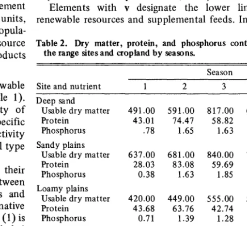
Model components H, J, and v are concerned with renewable resources. Elements within H give production rates in pounds of dry matter, protein, and phosphorus per acre of rangeland and cropland (Table 2) and the percentage of dry matter, protein and phosphorus per pound of supplemental feed (Table 3). Nutrient content of range forage and supplemental feeds were obtained from Cook and Harris (1968), Sims et al. (1971), and Morrison (1959). Each of the management alternatives modifies the production rate of the renewable resources. The model allows for the use of those management alternatives that contribute the greatest increase in the production output per unit cost.

Elements within J set out utilization rates of available dry matter, protein and phosphorus for the products under consideration. This set of cells is paired with the set of appropriate production rates in H. Entries in H are positive since they add to available dry matter, protein, and phosphorus. Entries in J are all negative since dry matter, protein, and phosphorus are used up in production. The accepted daily nutrient requirements for product outputs are shown in Table 4 (National Academy of Science, 1963).

Elements with v designate the lower limit of use of renewable resources and supplemental feeds. In this study, all

Table 2. Dry matter, protein, and phosphorus content (lb/acre) on the range sites and cropland by seasons.

Season

Site and nutrient 1 2 3 4 5

Deep sand

Usable dry matter 491.00 591.00 817.00 651.00 522.00

Protein 43.01 74.47 58.82 34.46 21.40

Phosphorus .78 1.65 1.63 1.11 0.47

Sandy plains

Protein 28.03 83.08 59.69 38.70 29.48

Phosphorus 0.38 1.63 1.85 1.32 0.55

Loamy plains

Protein 43.68 63.76 42.74 30.15 17.67

Phosphorus 0.71 1.39 1.28 0.66 0.36

Alfalfa cropland

Usable dry matter 3950.00 3950.00 3950.00

Protein 1000.00 1000.00 1000.00

Phosphorus 12.50 12.50 12.50

Sorghum cropland

Usable dry matter 1740.00 1740.00 1740.00 3354.00

Protein 138.00 138.00 138.00 265.20

(3)

Table 3. Dry matter, protein, and phosphorus content (%) of supplemental feeds.

Supplemental feeds Dry matter Protein Phosphorus

Cottonseed cake 94.0 25.0 0.99

Mineral block 0.0 0.0 6.00

Corn 97.0 6.0 0.40

Wheat 90.0 15.6 0.40

Beet pulp 91.0 1.6 0.10

entries in v were zero because the quantities consumed of dry matter, protein, and phosphorus were required to be less than or equal to the quantities available.

The quantity of product output requirements to be considered were listed in e. In this study, all cells within e contained zeros. This simply states that the model allowed the program to select whatever quantity of the various product outputs that resulted in maximum contribution margin from the use of the resource system. The only constraint was that no product could have a negative output value.

Elements within I link the product types to their quantity requirement (e) and to their gross revenues (g). M and N are groups of zeros needed to complete the total matrix of the management model.

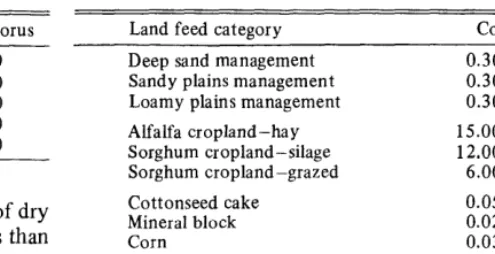
The final parts of the model make up the objective function. Elements within d designate the costs associated with each management alternative. In this study all management alternatives have only cost. The gross revenues were measured in final product output. Thus, the model is not concerned with maximizing dollar returns from any single management alternative but, instead, is concerned with management and dollar returns from the entire resource system. The costs listed in d are directly associated with managing an acre of rangeland per year, cultivating and/or harvesting acres of cropland per year, and the purchasing of supplemental feeds (Table 5).

The gross revenues associated with the product outputs are listed in g. The gross revenues are based on expected weight gains and expected sale prices for the various products during the various seasons (Table 6).

In this study, z denotes the maximum contribution margin. However, if the purpose was to allocate resources at the least probable cost to produce a specified quantity of product(s), z

Tables. Costs associated with management of rangeland, cultivating and/or harvesting cropland, and purchase of supplemental feeds.

Land feed category cost ($)I

Table 4. Livestock requirements for phosphorus, protein, and dry matter (lb/animal/season).

Product

Steer

Requirements Sea son Cow/calf Year-round Season 5 Season 1-4 Season 1-3

Phosphorus per season 1 2.25 1.35 1.35 1.35

2 2.25 1.31 1.31 1.31

3 3.00 1.74 1.74 1.74

4 1.50 0.87 0.87

5 5.40 3.60 3.60

Protein per season 1 103.50 58.50 58.50 58.50

2 103.80 67.50 67.50 67.50

3 138.00 90.00 90.00 90.00

4 69.00 45.00 45 .oo

5 252.00 234.00 234.00

Dry matter per season 1 1260.00 643.50 643.50 643.50

2 1260.00 859.50 859.50 859.50

3 1680.00 1146.00 1146.00 1146.00

4 840.00 573.30 573.30

5 3240.00 2268.00 2268.00

JOURNAL OF RANGE MANAGEMENT 27(3), May 1974

Deep sand management Sandy plains management Loamy plains management

Alfalfa cropland-hay Sorghum cropland-silage Sorghum cropland-grazed

0.30/acre/year 0.30/acre/year 0.30/acre/year

15.00/acre/year 12,00/acre/year 6.00/acre/year

Cottonseed cake Mineral block Corn Wheat Beet pulp

‘Based on 1971 prices.

O.O52/lb O.O27/lb O.O32/lb O.O25/lb O.O3O/lb

would denote the least cost. No matter what the purpose is in utilizing the resource system, fixed costs are incurred (Table 7). Whereas variable costs are adjusted for during the actual computing of the management plan, fixed costs must be adjusted for after the optimal management plan is selected. When we adjust the contribution margin for fixed costs, the resulting net dollar returns are, in fact, net revenues (net profits).

Management Plans

(4)

Table 6. Weights, prices, and gains of livestock and associated revenue from product sales.

Weight at Price/lb at Weight’ Weight Price/lb’ Gross

purchase purchase gain/day at sale at sale revenue

Product (lb) (cents) (lb) (lb) (cents) ($/head)

Calf 3 70 - 1.5 458 28.80 120.00

Steers-year round 500 25.36 1 s-1.7 1068 24.10 120.39

Steers-season 5 500 23.90 1.5 733 24.10 62.00

Steers-seasons l-4 500 25.36 1.7 812 23.90 63.08

Steers-seasons l-3 500 25.36 1.7 760 25.83 65.50

’ Averaged weight of all purchased stock.

2 Livestock prices are based on 1 l-year average (1959-1969). 3Each calf unit required feed from the mother cow.

resources and associated excess quantities of dry matter, protein, and phosphorus.

Output from the computer program indicated the maximum contribution margin under Plan I would be obtained by grazing 832 steers from October 1 to March 3 1 on 686 acres of sandy plains, 315 acres of unharvested sorghum cropland, and 90 acres of harvested alfalfa cropland. On April 1, all the steers would be sold and a new herd of 694 steers would be purchased. Their grazing schedule would be: April 1 to May 15, 164 acres of sandy plains, 29 1 acres of loamy plains and 56 acres of harvested alfalfa cropland; May 16 to June 30, 1,052 acres of deep sand; July 1 to August 3 1, 1,063 acres of deep sand. At the end of this period, the steers would be sold. The calculated contribution margin for the entire operation would be $92,003. When adjusted for $31,505 of fixed costs, the net profit would be $60,498.

need for a protein supplement to allow livestock (products) to utilize the excess dry matter. Cottonseed cake and wheat supplements had the highest percentage of protein; neverthe- less the program was allowed to select from all supplemental feeds (Table 1).

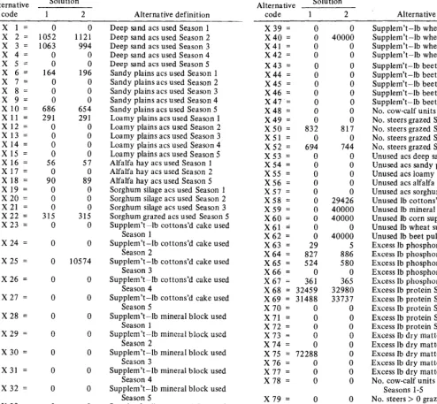
The slack variables for each resource constraint are helpful in explaining how management alternatives and product requirements are handled. X5 a - X, 7 are slack variables denoting the number of acres of rangeland and cropland left unused in the management plan (Table 8). In Plan I, X, a - X,, were all zero. This means that all available land acreage was used. X, s - Xb2 were slack variables that designated quantities of supplemental feed that were available but not used. In Plan I, X, a - Xb2 were all zero since no supplemental feeds were considered for use.

Variables X6 a - X,, showed that there was an excess of phosphorus, protein and/or dry matter in at least one of the five seasons. There was unused phosphorus in every season except Season 4. Seasons 1 and 2 had unused protein; and, there was excess dry matter in Season 3.

Whenever an excess of dry matter exists in a season, consideration should be given to use of supplemental feeds. An excess of dry matter denotes a shortage of nutrient in that particular season; i.e., a shortage of protein and/or phosphorus. Examination of slack variables in Season 3 showed an excess of phosphorus but not of protein. This suggested the

In Plan II constraints on supplemental feeds were arbitrarily set to be a maximum of 40,000 pounds. Cottonseed cake and wheat were the only supplemental feeds used in Season 3. With the use of supplemental feeds, output from the computer program indicated that maximum contribution margin would now be obtained by grazing 817 steers from October 1 to March 3 1 on 65 1 acres of sandy plains, 3 15 acres of unharvested sorghum cropland, and 89 acres of harvested alfalfa cropland. On April 1, all the steers would be sold and a new herd of 744 steers would be purchased. Their grazing schedule would be: April 1 to May 15, 199 acres of sandy plains, 291 acres of loamy plains, and 57 acres of harvested alfalfa cropland; May 16 to June 20, 1,128 acres of deep sand; July 1 to August 31,987 acres of deep sand; 10,574 pounds of cottonseed cake supplement, and 40,000 pounds of wheat supplement. For Plan II, the grazing herds would be assigned to pastures as shown in Figure 2. At the end of the summer

II

294 Acres Sandy Plotns Season 5

I I l-

’ IS6 Acres 1 Sandy Plains

, Season I ₂₉₁ _Acrea Loamy Plolns Season

I

562 Acres Deep Sand Season 2

55 _\ 315 Acres

I66 Acres Deep Sand Season 2

69 Acres Alfolfo Hoy Season 5 \ 57 Acres

J

Table 7. List of fixed costs for management of Akron Ranch.

Item Cost ($)

Depreciation on equipment and buildings (1 O%/year) 2,610

Repairs, gas, oil for vehicles 1,500

Labor: Manager for Akron Ranch 15,000

Hired hand (75% of $5,00) 3,750

Water development 680

Veterinarian expenses 2,200

Rental on land 1,886

Taxes 2,352

Transportation costs for livestock 927

Miscellaneous 600

Total fixed costs $31,505

---

302 ! 205 q 372 Acres

Deep Sand Season 3

Acres I Acres

Deep 1 Sandy - Orglnal Fence Sand I Platns --- New Fence Season 3 1 Season 5

320 Acres Deep Sand Season 3

Fig. 2. Pasture plan for the Eastern Colorado Range Station, Akron,

(5)

Table 8. Results from computer program executions-list of 82 variables in two management plans for the Eastern Colorado Range Station.’

Alternative Solution

code 1 2 Alternative definition

x

l= 0

x 2 = 105; 1121 X 3 = 1063 994

x 4= 0 0

x 5= 0 0

X 6= 164 196

x 7= 0 0

X 8= 0 0

x 9= 0 0

x10 = 686 654 x11 = 291 291

x12 = 0 0

x13 = 0 0

x14 = 0

x15 = 0 0”

Xl6 = 56 57

x17 = 0 0

Xl8 = 90 89

x19 = 0 0

x20 = 0 0

x21 = 0 0

x22 = 315 315

X23 = 0 0

X24 = 0 0

X25 = 0 10574

X26 = 0 0

X27 = 0 0

X28 = 0 0

x29 = 0 0

x30 = 0 0

x31 = 0 0

X32 = 0 0

x33 = 0 0

x34 = 0 0

x35 = 0 0

X36 = 0 0

x37 = 0 0

X38 = 0 0

Deep sand acs used Season 1 Deep sand acs used Season 2 Deep sand acs used Season 3 Deep sand acs used Season 4 Deep sand acs used Season 5 Sandy plains acs used Season 1 Sandy plains acs used Season 2 Sandy plains acs used Season 3 Sandy plains acs used Season 4 Sandy plains acs used Season 5 Loamy plains acs used Season 1 Loamy plains acs used Season 2 Loamy plains acs used Season 3 Loamy plains acs used Season 4 Loamy plains acs used Season 5 Alfalfa hay acs used Season 1 Alfalfa hay acs used Season 2 Alfalfa hay acs used Season 5 Sorghum silage acs used Season 1 Sorghum silage acs used Season 2 Sorghum silage acs used Season 3 Sorghum grazed acs used Season 5 Supplem’t-lb cottons’d cake used

Season 1

Supplem’t-lb cottons’d cake used Season 2

Supplem’t-lb mineral block used Season 1

Supplem’t-lb corn used Season 1 Supplem’t-lb corn used Season 2 Supplem’t-lb corn used Season 3 Supplem’t-lb corn used Season 4 Supplem’t -lb corn used Season 5 Supplem’t-lb wheat used Season 1

Alternative Solution

code 1 2 Alternative definition

x39 = 0

x40 = 0 x41 = 0 X42 = 0

x43 = 0 x44 = 0 x45 = 0 X46 = 0 x47 = 0 X48 = 0 x49 = 0 x50 = 832 x51 = 0 x52 = 694 x53 = 0 x54 = 0 x55 = 0 X56 = 0 x57 = 0 X58 = 0 x59 = 0 X60 = 0 X61 b 0 X62 = 0 X63 = 29 X64 = 827 X65 = 524 X66 = 0 X67 = 361 x 68 = 32459 X69 = 31488 x70 = 0 x71 = 0 X72 = 0 x73 = 0 x74 = 0 X 75 = 72288 X76 = 0 x77 = 0 X78 = 0

x79 = 0

X80 = 832

X81 = 0

X82 = 694

0 40000 0 0 0 0 0 0 0 0 0 817 0 744 0 0 0 0 0 29426 40000 40000 0 40000 886 580 0 365 32980 33737 0 0 0 0 0 0 0 0 0

0 No. steers > 0 grazed Seasons l-5 817 No. steers > 0 grazed Season 5

0 No. steers > 0 grazed Seasons l-4 744 No. steers > 0 grazed Seasons l-3

Supplem’t-lb wheat used Season 2 Supplem’t-lb wheat used Season 3 Supplem’t-lb wheat used Season 4 Supplem’t-lb wheat used Season 5

Supplem’t-lb beet pulp used Season 1 Supplem’t-lb beet pulp used Season 2 Supplem’t-lb beet pulp used Season 3 Supplem’t-lb beet pulp used Season 4 Supplem’t-lb beet pulp used Season 5 No. cow-calf units grazed Seasons l-5 No. steers grazed Seasons l-5 No. steers grazed Season 5 No. steers grazed Seasons l-4 No. steers grazed Seasons l-3 Unused acs deep sand Unused acs sandy plains Unused acs loamy plains Unused acs alfalfa Unused acs sorghum

Unused lb cottons’d cake supplem’t Unused lb mineral block supplem’t Unused lb corn supplem’t Unused lb wheat supplem’t Unused lb beet pulp supplem’t Excess lb phosphorus Season.1 Excess lb phosphorus Season 2 Excess lb phosphorus Season 3 Excess lb phosphorus Season 4 Excess lb phosphorus Season 5 Excess lb protein Season 1 Excess lb protein Season 2 Excess lb protein Season 3 Excess lb protein Season 4 Excess lb protein Season 5 Excess lb dry matter Season 1 Excess lb dry matter Season 2 Excess lb dry matter Season 3 Excess lb dry matter Season 4 Excess lb dry matter Season 5 No. cow-calf units > 0 grazed

Seasons l-5

‘Contribution margin (or maximum objective) = $92,003 for Solution

1 and $92,781 for Solution 2.

period the steers would be sold. The calculated contribution margin for Plan II would be $92,781. Again, adjusting for $31,505 of fixed costs, the net profit would be $61,276.

Discussion

Based on the assumption of known information, two possible management plans were determined for the Eastern Colorado Range Station (ECRS). In Plan I, when no supplemental feeds were used, net revenue was $60,498. Making use of supplemental feeds in Plan II resulted in net revenue of $61,276. Based on the objective of profit maximization, Plan II is the optimal management plan with an additional net revenue of $778.

Dollarwise the advantage of using Plan II is very slight. Therefore, the land manager must examine further the effect of using supplemental feeds with respect to re-allocation of land use over the various seasons. The effect of re-allocation

(6)

Literature Cited co. 1147 p.

Cook, C. Wayne, and L&n E. Harris. 1968. Nutritive value of seasonal National Academy of Science. 1963. Nutrient requirements of beef cat- ranges. Agr. Exp. Sta. Bull. 472. Utah State Univ., Logan. 55 p. tle. National Research Council. Pub. No. 1137. 32 p.

D’Aquino, Sandy A. 1972. Programming for optimum allocation of Sims, P. L., and A. H. Denham. 1969. Eastern Colorado Range Station resources: Eastern Colorado Range Station. PhD. Diss., Colo. State climatic data, 1956-1968. Prog. Rep. 6945, Agr. Exp. Sta., Colo-

Univ., Fort Collins. 244 p. rado State Univ., Fort Collins. 3 p.

Farm Credit Bank of Wichita. 1969. Kansas City livestock prices Sims, P. L., G. R. Loveli, and D. F. Hervey. 1971. Seasonal trends in 1959-69. Research Division, Wichita, Kansas. herbage and nutrient production of important sandhill grasses. J. Morrison, H. B. 1959. Feeds and feeding. Clinton, Iowa: Morrison Publ. Range Manage. 24:55-59.

A Serial

Optimization

Model for Ranch

Management

E. T. BARTLETT, GARY R. EVANS, AND R. E. BEMENT Highlight: A linear program resource management model is

described. This model is used to aid in the decision-making process of developing basic ranch management plans. A simple

one-year-at-a-time ranch management plan for the Central

Plains Experimental Range was developed. The model uses

discrete continuity equations to facilitate the flow of resources and products through seasons of the year. Management strate- gies based on the amount of initial operating capital ($20,000

to unlimited) are discussed.

Managers in business and industry are continually charged with making decisions concerning the efficient allocation of scarce resources. The economic existence of ranchers is based on efficiency. They must allocate their resources among alternative range products, such as cows and calves or yearlings, and must determine when and how best to use the resources. All these decisions affect economic resource allocation and are confounded by a myriad of alternative practices available to ranchers. It would be desirable to have a management technique that would compare alternatives and provide a quantitative guide for the rancher. Linear programming appears to be such a tool.

Linear programming is a mathematical optimization technique for allocating scarce or fixed resources to management alternatives. It consists of a set of linear equations which explicitly express, in mathematical terms, the limited resources, the management alternatives, and the decision-maker’s objective. Simply stated, “the objective in linear programming is to maximize or minimize a linear function subject to a number of linear constraints (Clough, 1963)“. The resulting optimum solution yields a set of computer decision guides for the resource manager to consider in relation to other nonquan-

The authors are assistant professor, Department of Range Science, Colorado State University, Fort Collms; range conservationist, U.S. Department of Agriculture, Soil Conservation Service and senior agency cooperator, Regional Systems Program, Colorado State University, Fort Collins; and range scientist, Agricultural Research Service, U.S. Dep. Agr., Fort Collins, Colorado.

This research is supported by NSF Grant No. G11333370 through the Regional Analysis of Grassland Environmental Systems Program at Colorado State University. RANGES Report No. 4 and Colorado State University Experiment Station (Scientific Series Number 1834).

Manuscript received April 11, 197 3.

tified variables before selecting his final decision. Static linear programming models can only consider alternatives in a single time period. Serial linear programming models, as used in this paper, can consider an alternative in one time period in relation to an alternative in a previous time period. This relationship between static and serial models will be discussed in later sections of the paper.

This paper presents an example of how linear programming can be applied to ranching decisions and provides a guide to application in other resource management fields. In addition to static decisions in which all components are considered fixed, a serial linear model is presented which allows for seasonal growth of vegetation, the buying and selling of livestock, and cash flow of income and costs.

Dantzig (195 1) developed the linear programming technique shortly after World War II, and it was rapidly applied to problems in business. This method was successfully applied to agricultural problems before 1960 (Heady and Candler, 1958; Candler, 1956). Only during the past decade has linear programming been applied to natural resources. Nielsen and others (1966) used this technique in their study of federal range use and improvement for livestock production. Other workers developed models for multiple use of federal lands (Bell, 1970; Navon, 1967). D’Aquino (1972,1974) developed a general resource allocation model using linear programming and applied this to a hypothetical ranching operation. D’Aquino’s model, however, was static with respect to the range resources. Consequently, if an acre of resource was used at one time, it could not be used again. The results of D’Aquino’s model and a serial model will be compared.

Study Area

Central Plains Experimental Range (CPER), totaling 15,700 acres, was used as an operating ranch. It is about 25 miles south of Cheyenne, Wyoming, and 12 miles northeast of Nunn, Colorado, in the central part of the Northern Great Plains shortgrass area. Annual precipitation ranges from 10 to 15 inches, with a summer (April-Sept.) mean of 10.17 inches and a winter mean (October-March) of 2.18 inches (Bertolin,

1970). The mean elevation of the area is 4,700 ft above sea