The Solution Of Large System Of Linear Equations By Using Several Methods And Its Applications

The Solution of Large System of Linear Equations by using

several Methods and its applications.

Md. Noor-A-Alam Siddiki

Department of Natural Science, Stamford University Bangladesh.

[email protected]

Abstract

The Significance of linear system of equations has many problems in engineering and different branches of sciences. To solve the system of linear equations, there have many direct or indirect methods. Gaussian elimination with backward substitution is one of the direct methods. This method is still the best to solve the linear system of equations. Gauss-Jordan method is a simple modification of Gaussian elimination method. Iterative improvement method is used to improve the solution. Our aim is to solve a large system developing several types of numerical codes of different methods and comparing the result for better accuracy. We also represent some practical field where the system of linear equations is applicable.

Keywords: Gaussian elimination method, Gauss-Jordan method,

Iterative improvement method,, applications24T.

1. Introduction

There are many physical and numerical problems in which the solution is obtained by solving a set of linear system of equations. These problems can be a fairly simple one, when the number of unknowns is small, and is often studied at elementary level in mathematics. The problem has a unique solution when there are

n

linearly independent equations and

n

unknowns.

Practical methods for the solutions of the systems of linear equations fall into two main classes. These methods are particularly suited for computers. The two methods are commonly known as the (1) Direct methods and (2) Indirect methods. In direct methods, in principle, a simple application of a manipulative process suffices to give an exact solution. This method is based on the elimination of variables to transform the set of equations to a triangular form. In indirect methods generally make repeated use of a rather simpler type of process to obtain successively improved approximations to the solution. Each one of these methods has its advantages and an understanding of the methods is needed to a judicious choice when a set of equations is given. Even though a direct methods is designed to produce an exact solution, the limitations of computers make this an unattainable goal in errors have the least possible effect on the final answer, and we pay due attention to this matter in what follows:

We point that the following types of problem lead to systems of linear equations:

Problems in mechanics that involve designing functions, columns, arches, bridges and other structures.

Problems in geodesy connected with making maps from given geodesic photographs. The systems involved contain many unknowns, often numbering in the hundreds.

Problems of finding the values of coefficients in empirical formulas. A basic method here is that of using systems linear equations.

Problems of solving equations approximately (these are common in higher mathematics).

Problems in newest areas of physics and related sciences, such as the theory of relativity, atomic physics, and meteorology, solid state physics, make extensive use of systems of linear equations.

Numerical linear algebra, as the name implies, consists of the study of computational algorithms for solving problems for in linear algebra. It is very important subject in numerical analysis because linear problems occur so often in applications. It has been estimated, for example, that 75% of all scientific problems require the solution of linear equations at one stage or another. It is therefore important to solve linear problems efficiently and accurately.

Therefore, the linear systems of equations are associated with many problems in engineering and sciences as well as with applications of mathematics to the sciences and the quantitative study of business and economic problems.

Gaussian elimination with backward substitution procedure is one of the direct methods for solving the system of linear equation as

Ax

=

b

.

The method is based ultimately on the process of elimination of variables. It is convenient to suppress all unnecessary symbols and to operate upon at array composed entirely of numerical elements. Such an array is called augmented matrix. Gaussian elimination reduces a matrix not all the way to the identity matrix, but only halfway, to a matrix whose components on the diagonal and above remain nontrivial. The combination of Gaussian elimination and back substitution yields a solution to the set of equation. In this procedure, if any element of the main diagonal is zero, then row interchange is performed.

Scaled-column pivoting procedure is simply modification of the partial column pivoting. This process is necessary sometimes to obtain accurate result of the system.

The Gauss-Jordan method is another well-known procedure for solving a linear system of equations. It is the same as Gaussian elimination with the modification that elimination is done above the diagonal as well as below. In other words, it reduces the problem

Ax

=

b

to the equivalent one

Dx

=

q

, where

D

is a diagonal matrix. Thus, the reduced problem is especially easy to solve. For inverting matrix, Gauss-Jordan elimination is about as efficient as any other method.

Another procedure of Gauss-Jordan method is based on the interchanging rows and columns (full pivoting). In this method, elimination uses one or more of the full pivoting to reduce the matrix

[ ]

A

to the identity matrix. When this is accomplished, the right-hand side becomes the solutions.

Iterative improvement of the solution to

Ax

=

b

, The first guess

x

+

δ

x

is multiplied by

A

to produce

b

+

δ

b

. The known vector

b

is subtracted, giving

δ

b

. The linear set with this right-hand side is inverted, giving

δ

x

. This subtracted from the first guess gives an improved solution

x

.

It is apparent that iterative improvement can be very useful. For well-conditioned systems, it provides peace of mind in that it gives assurance that Gauss elimination has produced good solution; for less well-conditioned problems, one or two iterations will give a better solution; while for badly conditioned systems, it can inform us of the fact so that an appropriate remedy can be taken rather than proceed with the overall computations using an incorrect result.

2. Several Direct and iterative improvement

methods:

2.1

1 System of linear equations and augmented

matrix

:

A system of linear algebraic equations in

n

unknowns

(

i

n

)

x

_i

,

=

1

,

2

,

3

,



,

is usually written in the form:

n

n

nn

n

n

n

n

n

n

b

x

a

x

a

x

a

b

x

a

x

a

x

a

b

x

a

x

a

x

a

=

+

+

+

=

+

+

+

=

+

+

+





















2

2

1

1

2

2

2

22

1

21

1

1

2

12

1

11

( )

2

.

1

the system

( )

2

.

1

can be written as

AX

=

B

where

A

is the matrix of coefficients,

X

is a column vector whose elements

are

x

_i

,

(

i

=

1

,

2

,

3

,



,

n

)

and

B

is also a column vector whose elements are

b

_i

,

(

i

=

1

,

2

,

3

,



,

n

)

that is

A

=

[ ]

a

_ij

,

[ ]

x

_i

X

=

,

B

=

[ ]

b

_i

. Combining the matrices

A

&

B

, we get augmented matrix such as

W

=

[ ]

A

,

B

=

[

a

_ij



b

_i

]

2.2

Gaussian Elimination method:

Gaussian elimination method is one of the several of the direct methods. This method is a systematic elimination procedure whose object is the transformation of an initial rectangular system of equations into a triangular system, which we can solve easily. From system

( )

1

.

1

we have

Ax

=

b

and augmented matrix is

W

=

[ ]

A

,

b

, applying elementary row operation we obtain a triangular form

d

Ux

=

where

U

is an

n

×

n

upper triangular matrix. The equivalent linear system in the triangular form as

1 , 1 , 2 2 2 22 1 , 1 1 2 12 1 11 + + +

=

=

+

+

=

+

+

+

n n n nn n n n n n n

a

x

a

a

x

a

x

a

a

x

a

x

a

x

a

















by backward substitution we get,

x

_n

=

a

_n,n+1

a

_nn ,

(

n n n n n

)

nn

n

a

a

x

a

x

₋₁

=

_{−1, +1}

−

_−1,

in general, _{j ii}

n i j ij n i

i

a

a

x

a

x

_















−

=

∑

+ = + 1 1

, for each

.

1

,

2

,

3

,

,

2

,

1

−





−

=

n

n

i

two pivoting strategy is related to Gaussian elimination method that’s are partial pivoting and scale partial pivoting. To remove round-off error; namely rounding errors, both strategies are used.

2.3 Gauss-Jordan method:

we have to extend the elimination processes of the Gauss method so that the final form of the augmented matrix after elimination is a diagonal matrix. Each equation has only one variable, so that we can calculate the values of the variables directly. The corresponding augmented matrix of the system

( )

2

.

1

can be written after applying G-J

method as

( )

( )

( )

( )

( )

( )

































=

+

+

+

n

n

n

n

n

n

n

n

a

a

a

a

a

a

W

1

,

,

2

1

,

2

2

22

1

1

,

1

1

11

0

0

0

0

0

0



























the

2.4 Another process of Gauss-Jordan method:

This method is based on the elimination on the column-augmented matrices and complete or full pivoting. Complete pivoting may require both row and column interchanges. For inverting a matrix, Gauss-Jordan elimination is about efficient as any other method. For clarity, and to avoid writing endless ellipses we will write out equations only for the case of four equations and four unknowns, and with three different right-hand side vectors that

are known in advance. For this case,

x

_ij

is the

i

th component

(

i

=

1

,

2

,

3

,

4

)

of the vector solution of the

j

th

right-hand side

(

j

=

1

,

2

,

3

)

, the one whose coefficients are

b

_ij

,

i

=

1

,

2

,

3

,

4

;

and that the matrix of unknown coefficients

y

_ij

is the inverse matrix of

a

_ij

.

In words, the matrix solution of

[ ][

A

.

x

₁

∪

x

₂

∪

x

₃

∪

Y

] [

=

b

₁

∪

b

₂

∪

b

₃

∪

1

]

where

A

and

Y

are square matrices, the

b

_i

'

s

and

x

_i

'

s

are column vectors, and

1

is the identity matrix, simultaneously solves the linear sets

3

3

2

2

1

1

.

.

.

x

b

A

x

b

A

x

b

A

=

=

=

and

1

.

Y

=

A

We must do never do Gauss-Jordan elimination without pivoting. We do full pivoting in the routine in this section.

2.5 Iterative improvement of a solution to linear

equations:

Suppose the linear system is

A

.

x

=

b

( )

2

.

2

And a vector

x

is the exact solution of this linear system. We don’t however know

x

. We only know some slightly wrong solution

x

+

δ

x

, where

δ

x

denote the unknown error, when multiplied by the matrix

A

, slightly discrepant from the desired right-hand side

b

,

Namely,

A

.

(

x

+

δ

x

)

=

b

+

δ

b

( )

2

.

3

Subtracting

( )

2

.

2

from

( )

2

.

3

we have,

A

.

δ

x

=

δ

b

( )

2

.

4

But

( )

2

.

3

can also be solved, trivially, for

δ

b

, substituting this into

( )

2

.

4

we get,

A

.

δ

x

=

A

.

(

x

+

δ

x

)

−

b

( )

2

.

5

Since

x

+

δ

x

is the wrong solution that we want to improve. We need only solve

( )

2

.

5

for the error

δ

x

, then subtract this from the wrong solution to get an improved solution.

3. Arithmetical operations and Numerical

Implementation:

3.1 Number of arithmetical operations:

The number of divisions, multiplications, additions, subtractions and recordings of intermediate results provides a very rough estimate of the efficiency of an algorithm. For each direct method and for each step of an iterative method it is possible to estimate the numbers of these operations as functions of

n

, the order of the matrix. Here we represent the total arithmetic operations of several direct methods and iterative improvement method on the table.

Table

Total number of arithmetic operations (For

n

×

n

matrix)

Name of the method

Multiplications/Di visions

Additions/Subtra ctions

Total number of Arithmet ical operation s Gaussian

Eliminati on

method

3

3

2

3

_n

_n

n

+

−

6

5

3

2

n

3

+

n

2

−

3

3

n

≈

Gauss-Jordan Eliminati on method

n

n

n

2

1

2

1

_{3 2}

−

+

n

n

2

1

2

1

₃

−

2

3

n

≈

Iterative Improve ment of a solution to linear equations

2

n

3.2 Numerical Implementation:

We have developed some routine for solving the algebraic system of linear equations. The method that that is one of the oldest, and still perhaps the best, for the treatment of linear system is known as Gaussian elimination with backward substitution. Its corresponding pivoting strategy routine is known as maximal column pivoting or partial pivoting and Gaussian elimination with scaled-column pivoting.

To avoiding the round-off errors and for improving the solution, we develop the routine based on iterative Improvement of a solution to linear equations.

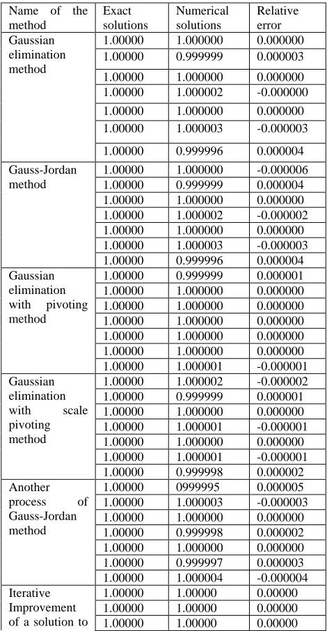
For various routines, we find-out the numerical solutions; compare these solutions with the exact known solutions whenever available, we also show the relative error. At first we have taken a

7

×

7

matrix with right hand-side quantities of the large systems whose exact solutions is known, forming augmented matrix, we carry out the numerical solutions using various routines. Comparing these numerical solutions with the exact solutions we represent the relative error on the table

( )

1

.

1

below:

Table 1.1

Name of the method

Exact solutions

Numerical solutions

Relative error Gaussian

elimination method

1.00000 1.000000 0.000000 1.00000 0.999999 0.000003 1.00000 1.000000 0.000000 1.00000 1.000002 -0.000000 1.00000 1.000000 0.000000 1.00000 1.000003 -0.000003

1.00000 0.999996 0.000004 Gauss-Jordan

method

1.00000 1.000000 -0.000006 1.00000 0.999999 0.000004 1.00000 1.000000 0.000000 1.00000 1.000002 -0.000002 1.00000 1.000000 0.000000 1.00000 1.000003 -0.000003 1.00000 0.999996 0.000004 Gaussian

elimination with pivoting method

1.00000 0.999999 0.000001 1.00000 1.000000 0.000000 1.00000 1.000000 0.000000 1.00000 1.000000 0.000000 1.00000 1.000000 0.000000 1.00000 1.000000 0.000000 1.00000 1.000001 -0.000001 Gaussian

elimination

with scale pivoting

method

1.00000 1.000002 -0.000002 1.00000 0.999999 0.000001 1.00000 1.000000 0.000000 1.00000 1.000001 -0.000001 1.00000 1.000000 0.000000 1.00000 1.000001 -0.000001 1.00000 0.999998 0.000002 Another

process of Gauss-Jordan method

1.00000 0999995 0.000005 1.00000 1.000003 -0.000003 1.00000 1.000000 0.000000 1.00000 0.999998 0.000002 1.00000 1.000000 0.000000 1.00000 0.999997 0.000003 1.00000 1.000004 -0.000004 Iterative

Improvement of a solution to

1.00000 1.00000 0.00000 1.00000 1.00000 0.00000 1.00000 1.00000 0.00000

linear equations

1.00000 1.00000 0.00000 1.00000 1.00000 0.00000 1.00000 1.00000 0.00000 1.00000 1.00000 0.00000

As a sample, we have taken matrix as large as 50 x 50 of the coefficients of unknown of a system of linear equations of order fifty with right-hand side constants whose exact solution is unknown. We represented here the numerical solutions, solving by UGaussian Uelimination with backward substitution method and

its corresponding partial pivoting, scale-partial pivoting and Gauss-Jordan method

1.412848 -3.139083

-1.926042

-0.434902

-2.019750

1.787170 4.114847

-2.905257 0.467713 3.472563

-2.563707

-0.031240

-2.594952 1.984129 -1.065152

2.143230

-1.800176 1.258903 0.025634 1.927285

-1.222465

-1.938268 0.865447 1.450536 -0.089902

-1.295377

-0.251918

-1.698674 0.154153 -0.156411

0.998276 0.551190 2.825744 0.698738 -2.817550

-0.994950 0.072627 0.582780 1.580843 -2.527471

2.152236

-0.802919 1.053731 1.843399 1.592495

0.713390 1.681474 1.340143 -0.695032

-1.279316

4. Applications of system of linear equations:

nodes, and directed lines connecting some or all of the nodes. The flow is indicated by a number or variable. We observe the following basic assumptions:

The total flow into a node is equal to the flow out of a node. The total flow into the network is equal to the total flow out of the network.

The picture below represents a system of one way streets in a particular part of some city and the traffic flow along the streets between the junctions:

We first equate the total flow into each node with the total flow out of the same node:

Node A:

200

+

x

₃

=

x

₁

+

x

₂

Node B:

200

+

x

₂

=

300

+

x

₄

Node C:

400

+

x

₅

=

300

+

x

₃

Node D:

500

+

x

₄

=

300

+

x

₅

We then equate the total flow into and out of the network:

300

300

300

500

200

200

400

+

+

+

=

+

+

x

₁

+

These give rise to a system of

5

linear equations

400

200

100

100

200

1

5

4

5

3

4

2

3

2

1

=

−

=

−

=

=

=

−

+

x

x

x

x

x

x

x

x

x

x

We have general solution

(

x

₁

,

x

₂

,

x

₃

,

x

₄

,

x

₅

) (

=

400

,

t

−

100

,

t

+

100

,

t

−

200

,

t

)

, where

t

is a parameter.

4.2 Application to Electrical Networks:

A simple electric circuit consists of two basic components, electrical sources where the electrical potential

E

is measured in volts

( )

V

, and resistors where the resistence

R

is measured in ohms

( )

Ω

. We are interested in determining the current

I

measured in amperes

( )

A

. The current flow in an electrical circuit is governed by three basic rules that are Ohm’s law, Current law and Voltage law.

Consider the electric circuit shown in the diagram below:

+ - 16 V +

20 V - Loop 1

Loop

2 20 Ω 8 Ω

4 Ω

I3

I1

I2

A

B

Outer loop

We wish to determine the currents

I

₁

,

I

₂

and

I

₃

. Applying the current law to the point

A

, we obtain

I

₁

=

I

₂

+

I

₃

.

Applying the current law to the point

B

, we obtain the same. Next let us consider the left hand loop, the voltage law applied to this loop now gives

8

I

₁

+

4

I

₂

−

20

=

0

.

Next, let us consider the right hand loop, the voltage law applied to this loop now gives

0

16

4

20

I

₃

−

I

₂

−

=

.

We now have a system of three linear equations

4

5

5

2

0

3

2

2

1

3

2

1

−

=

−

=

+

=

−

−

I

I

I

I

I

I

I

The solution is

I

₁

=

2

and

I

₂

=

I

₃

=

1

.

4.3 Application to Economics:

We describe a simple exchange model due to the economist Leontief. An economy is divided into sectors. We know the total output for each sector as well as how outputs are exchanged among the sectors. The value of the total output of a given sector is known as the price of the output. Leontif has shown that there exist equilibrium prices that can be assigned to the total output of the sectors in such a way that the income for each sector is exactly the same as its expenses.

Proportion of output from sector

A

B

C

Purchased by sector

A

0.2 0.6 0.1

Purchased by sector

B

0.4 0.1 0.5

Purchased by sector

C

0.4 0.3 0.4

Let

x

_A

,

x

_B

,

x

_C

denote respectively the value of the total output of sectors

A

,

B

,

C

. For the expense to match the value for each sector, we must have

,

4

.

0

3

.

0

4

.

0

,

5

.

0

1

.

0

4

.

0

,

1

.

0

6

.

0

2

.

0

C

C

B

A

B

C

B

A

A

C

B

A

x

x

x

x

x

x

x

x

x

x

x

x

=

+

+

=

+

+

=

+

+

leading to the homogeneous linear equations

,

0

6

.

0

3

.

0

4

.

0

,

0

5

.

0

9

.

0

4

.

0

,

0

1

.

0

6

.

0

8

.

0

=

−

+

=

+

−

=

−

−

C

B

A

C

B

A

C

B

A

x

x

x

x

x

x

x

x

x

leading to the solution

(

)













=

,

1

12

11

,

16

13

,

,

x

x

t

x

_{A B C} ,

where

t

is a real parameter.

4.4 Application to Chemistry:

Chemical equations consist of reactants and products. The problem is to balance such equations so that the following two rules apply: Conservation of mass and conservation of charge. Consider the oxidation of ammonia to form nitric oxide and water, given by the chemical equation

( )

x

₁

NH

₃

+

( )

x

₂

O

₂

→

( )

x

₃

NO

+

( )

x

₄

H

₂

O

.

Here the reactants are ammonia

(

NH

₃

)

and oxygen

( )

O

₂

, while the products are nitric oxide

( )

NO

and water

(

H

₂

O

)

. Our problem is to find out the smallest positive values of

4

3

2

1

,

x

,

x

,

x

x

such that the equation balances. To do this, the technique is to equate the total number of each type of atoms on the two sides of the chemical equation:

Atom N:

x

₁

=

x

₃

Atom H:

3

x

₁

=

2

x

₂

Atom O:

2

x

₂

=

x

₃

+

x

₄

These give rise to a homogeneous system of

3

linear equations

0

2

0

3

0

4

3

2

4

1

3

1

=

−

−

=

=

−

x

x

x

x

x

x

x

leading to the general solution

(

)













=

,

1

3

2

,

6

5

,

3

2

,

,

,

_{2 3 4}

1

x

x

x

t

x

where

x

₄

=

t

is a free

variable.

4.5 Application to Mechanics: We consider the problem of systems of weights, light ropes and smooth light pulleys, subject to the following two main principles: (i) if a light rope passes around one or more smooth light pulleys, then the tension at the two ends are the same (ii) Newton’s second law of motion: we

have

..

x

m

F

=

, where

F

denotes force,

m

denotes mass and

..

x

denotes acceleration.

Two particles, of mass

2

and

4

(kilograms), are attached to the ends of a light rope passing around a smooth light pulley suspended from the ceiling as shown in the diagram below:

Here

T

denotes the tension in the rope, and

g

denotes acceleration due to gravity. Newton’s laws of motion applied to the two particles then give the equations

T

g

x

T

g

x

=

2

−

&

4

=

4

−

2

..

..

.

We also have the conservation of the length of the rope, in the

form

x

₁

+

x

₂

=

C

, so that

0

..

2

..

1

+

x

=

x

. We have the system of linear equations:

0

,

4

4

,

2

2

..

2

..

1

..

2

..

1

=

+

=

+

=

+

x

x

g

T

x

g

T

x

this leads to the solution











−

=













g

g

g

T

x

x

3

8

,

3

1

,

3

1

,

,

..

2 ..

1

5. Conclusion:

We have developed the standard routine for Gaussian elimination method with backward substitution and its corresponding pivoting strategy, Gauss-Jordan method, and Iterative Improvement method. We solve several linear systems of equations using those developing methods. Large matrices arise in the large system equations. We have found numerical solution to a comparatively large system (where

50

×

51

an augmented matrix arises) by several methods. We compare the numerical solutions with the exact solutions for a system (where

7

×

8

augmented matrix arises) by several developing routine. We tabulated total number of arithmetical operations. Our special attention to the applications of system of linear equations in different branches of science and business area.

References:

[1] PRESS, W.H., FLANNERY, B.P., TEUKOLSKY, S.A. and VETTERLING W. T. Numerical Recipes: the art of scientific computing, Cambridge University Press, Chapter 2, 1990.

[2] BURDEN, R.L., FAIRES J.D., and REYNOLDS A.C., Numerical Analysis, Prindle, Weber and Schmidt, Boston, 1981.

[3] JOHNSTON, R.L., Numerical Methods, A software approach, John Wiley and Sons, New York, 1982.

[4] W. W. L. CHEN, Linear algebra, Chapter 1, University of London, 1982, 2006.

[5] JOHNSON, L.W., and RIESS R.D., Numerical Analysis, Addision-wesly, Reading, MA, 1982.

[6] HOWARD ANTON, CHRIS RORRES, Elementary Linear Algebra, Applications Version, John Wiley and Sons, Inc.

[7] Z. BAI, M. FAHEY, AND G. GOLUB, Some large-scale matrix computation problems, J. Comput. Appl. Math., 74 (1996), pp. 71–89.

[8] M. BERRY AND G. GOLUB, Estimating the largest singular values of large sparse matrices via modified moments, Numer. Algorithms, 1 (1991), pp. 353–374.

[9] G. DAHLQUIST, S. C. EISENSTAT AND G. H. GOLUB, Bounds for the error of linear systems of equations using the theory of moments, J. Math. Anal. Appl., 37 (1972), pp. 151– 166.