A tractable closed form approximation of the ergodic rate in Poisson cellular networks

R E S E A R C H

Open Access

A tractable closed form approximation

of the ergodic rate in Poisson cellular

networks

Alexis I. Aravanis

, Thanh Tu Lam

, Olga Muñoz

, Antonio Pascual-Iserte

and Marco Di Renzo

Abstract

The employment of stochastic geometry for the analysis and design of ultra dense networks (UDNs) has provided significant insights into network densification. In addition to the characterization of the network performance and behavior, these tools can also be exploited toward solving complex optimization problems that could maximize the capacity benefits arising in UDNs. However, this is preconditioned on the existence of tractable closed form

expressions for the considered figures of merit. In this course, the present paper introduces an accurate

approximation for the moment generating function (MGF) of the aggregate other-cell interference created by base stations whose positions follow a Poisson point process of given spatial density. Given the pivotal role of the MGF of the aggregate interference in stochastic geometry and the tractability of the derived MGF, the latter can be employed to substantially simplify ensuing stochastic geometry analyses. Subsequently, the present paper employs the

introduced MGF to provide closed form expressions for the downlink ergodic capacity for the interference limited case, and validates the accuracy of these expressions by the use of extensive Monte Carlo simulations. The derived expressions depend on the density of users and base stations, setting out a densification road map for network operators and designers of significant value.

Keywords: Ultra dense networks, Poisson point process, Moment generating function, Interference, Ergodic capacity, Rate, Closed form, Base station density, User density

1 Methods/Experimental

The methods used in the present paper are based on the mathematical tools of random spatial processes and stochastic geometry. The analytical framework developed for the performance evaluation of ultra dense networks is validated by extensive Monte Carlo simulations.

2 Introduction

The advent of multimedia interactive services and the surge in the number of interconnected devices has imposed the investigation of new approaches able to enhance wireless capacity in 5G networks. In this course, three prime axes of network flexibility have been lever-aged, namely the employment of wider spectrum, the enhancement of spectral efficiency, and the employment

*Correspondence:[email protected]

1_{Department of Signal Theory and Communications, Universitat Politècnica de}

Catalunya (UPC), Barcelona, Spain

Full list of author information is available at the end of the article

of smaller cell sizes and, thus, of smaller transmit dis-tances. In retrospect over the evolution of wireless net-works, the efficient spatial reuse of the spectrum, through the reduction of the inter-site distances, has provided, out of these three axes of flexibility, the most substantial capacity gains by a large margin [1]. Hence, the densifica-tion of networks arises as the most prominent candidate for achieving the envisaged capacity increase in the 5G era as well.

In the direction of densifying their networks, network operators employ system-level simulations and network measurements. However, over the last decade, the seminal work of Baccelli et al. [2] gave rise to stochastic geom-etry as a tractable tool for the large-scale analysis and design of wireless networks. Indicatively, the formulation of tractable mathematical expressions for the expectation of the aggregate interference in wireless networks [3]— which was not analytically formulated hitherto—paved the way for the theoretical analysis of the performance of

wireless networks. Thenceforth, a multitude of research works exploited these tools to provide significant insights into network densification. These insights are essential for understanding the innate features of dense networks and can be employed by network operators as densifica-tion road maps and guidelines for the use of system level simulators and of auxiliary network planning tools.

The insights provided by such theoretical analyses brought about significant changes in the understanding of wireless networks. In particular, for single-slope path-loss models and for networks comprising significantly more users than base stations (BSs), it has been demon-strated that the user signal quality is independent of the BS density [4]. Moreover, the probability of coverage (which constitutes the complementary cumulative distribution function (CCDF) of the signal to interference plus noise ratio (SINR)) is independent of the BS density and of the number of tiers [5]. Similar analysis for the uplink (UL) has demonstrated that the UL signal to interference ratio (SIR) is also invariant of the BS density [6]. As a result, it has been demonstrated that the network capacity increases linearly with the density of BSs and with the number of tiers [3].

These conclusions, however, which indeed hold for sparse wireless networks (e.g., tier of macro cells (MCs)), do not hold for extremely high BS densities. The rea-son for that is that after a BS densification threshold, the inter-site distances become so small that the proximity of the neighboring BSs allows them to create line of sight (LOS) interference to the intended user. As a result, after this densification threshold, the probability of coverage is diminished precipitately due to the presence of LOS interference [7,8].

As opposed to this behavior of networks comprising much more users than BSs, the system performance is not bounded by the aforementioned threshold in the case of networks with more BSs than users; which is, in fact, the case of the envisaged UDNs [9]. The reason for that is that the excess BSs that do not serve any user can be switched off, thus, reducing the system energy consumption and interference. In this setup, the probability of coverage will still decrease when LOS interference first appears in the network, however, as the BS density increases past this point, the probability of coverage will increase again with the density of BSs. That is, since for a fixed number of users, the excess BSs will remain idle, and therefore will not create any interference, regardless of the density of BSs [10].

Based on this comprehensive analysis, it has become evident that two key factors need to be taken into account by network operators in order to tap the capacity potential of UDNs. Firstly, the detrimental effect of LOS inter-ference and, secondly, the beneficial effect of idle (i.e., non-transmitting) BSs. The incorporation of these two

effects in the design of UDNs could engender extraor-dinary capacity gains. In particular, the investigation of BS coordination schemes to counteract LOS interference could, indeed, allow for a linear capacity increase with the density of BSs. Besides, the coordination of only LOS interferers, able to communicate and coordinate directly with the intended user, would not require intricate coordi-nation schemes. Additionally, leveraging on the beneficial effect of the idle mode, users could be clustered dynami-cally under a single BS, not necessarily the one providing the best service to each user. Thus, BSs that were acting as sources of principal interference to the network could be switched off. Given the high density of BSs, the connec-tion to a neighboring BS after the best serving BS has been switched off would entail a minimal path-loss increase that would be outweighed by the interference mitigation gain achieved by strategically switching off BSs.

The development of mathematical frameworks for com-plex optimization problems, like the ones mentioned above poses a great challenge. The reason for that is that the majority of the stochastic geometry approaches in the literature, including the theoretical analyses presented above, involve intractable integrations. Even though such integrals can be computed numerically, allowing the anal-ysis of the network behavior, they cannot be employed for the investigation of complex optimization problems. In these cases, it is imperative that the considered objec-tive functions, which evaluate the system performance, involve tractable closed form expressions. In this course, it is essential to exploit the available stochastic geome-try tools to develop tractable and accurate approxima-tions in addition to the available exact but cumbersome expressions.

MGF imposed inherent limitations on the extension of the stochastic geometry analysis to complex optimization problems. However, the present paper lifts these inher-ent limitations by introducing a simple, albeit extremely accurate expression for the MGF of the other cell interference.

To elaborate, the main contributions of the present paper can be summarized as follows:

• Derivation of a tractable and extremely accurate approximation for the MGF of the aggregate other-cell interference. The aggregate interference is created by BSs whose spatial distribution follows a homogeneous Poisson point process (PPP).

• Extension of the MGF to account for two different scenarios. A realistic scenario where the fast fading characterizing the channels of the interferers is not known to the UE, and a scenario of academic interest, where the fast fading of the interferers can be taken into account.

• Derivation of a tractable and accurate approximation for the coverage probability in the interference limited and fully loaded case (i.e., forλUEλ). • Derivation of a tractable and accurate approximation

for the DL ergodic rate, in closed form, in the interference limited and fully loaded case.

• Derivation of a tractable and accurate approximation for the coverage probability in the interference limited but not fully loaded case (i.e., the case of the envisaged UDNs). As opposed to the fully loaded case, the coverage probability depends on the density of usersλUEand the density of BSsλ.

• Derivation of a tractable and accurate approximation for the DL ergodic rate, in closed form, in the interference limited but not fully loaded case. The closed form of the expressions and their dependence on the density of usersλUEand BSsλ, constitutes an invaluable figure of merit for network planning and network densification.

• The accuracy of the proposed approximations is validated through extensive Monte Carlo simulations, and the practicality of the derived expressions for future applications is outlined.

The remainder of the paper is organized as follows. Section3 presents the considered network architecture.

Section 4 presents the approximation for the MGF of

the aggregate other-cell interference in the DL. Section5 introduces for the first time in the literature closed form expressions for the ergodic rate in the DL for the interfer-ence limited case. Moreover, extensive simulation results are presented corroborating the accuracy of the derived expressions. Finally, Section 6 concludes the paper and presents perspectives.

3 The wireless cellular network

A wireless cellular system is considered, comprising a set of BSs, denoted by BSi, whose positionsxi ∈ R2follow a spatial distribution given by a homogeneous PPP of densityλ (BSs/m2). Moreover, the positions of the over-laid user equipment (UE) follow also a spatial distribution given by a homogeneous PPPof densityλUE(UE/m2). The reference UE, denoted by UE0, is located at the ori-gin and is served by its closest BS, denoted by BS0. The UE adjoined at the origin can be singled out and the loca-tion of the other UE follows the reduced Palm distribuloca-tion of, which is the same as the original distribution(as stated by Slivnyaks theorem [12]). Hence, adjoining UE0at the origin does not change the distribution of.

For the sake of simplicity in the notation, it is assumed that all UE and BSs are equipped with one antenna and all BSs transmit at the same power level. Intra cell users are assumed to be sharing orthogonal resources, as is typically the case in the literature [6], whereas all BSs use the same frequency band. If not explicitly mentioned otherwise (as will be done in the following sections), it is assumed that the network comprises significantly more users than BSs (i.e.,λUE λ). As a result, every BS is active and trans-mitting, acting as an interferer in the DL. The other-cell interference in the DL is mathematically defined as the interference coming from all BSs residing at a distance ||xi||from the origin greater than the distance||x0||of BS0 from the origin, where||·||denotes thel2-norm. Note that the origin is where the reference UE UE0is located. Last but not least, a single-slope unbounded path-loss model is assumed in the analysis.

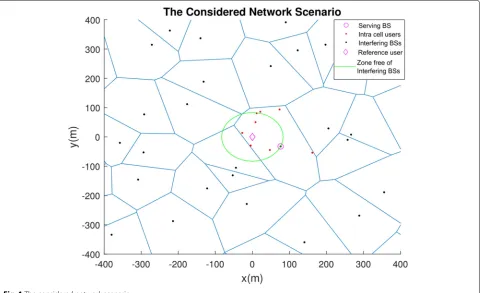
The considered scenario is depicted in Fig. 1. UE0 is

marked by the magenta diamond, BS0 by the magenta

circle, and the intra cell users are depicted in red. The interfering BSs are depicted in black and reside in dis-tances (||xi|| > ||x0||), where the circle of radius ||x0|| around UE0 is depicted in green. Every BS residing in the region outside this circle is acting as an interferer in the DL.

4 MGF of the aggregate other-cell interference Having presented the considered network scenario and having defined the set of interfering BSs by means of their distance to the origin, we can proceed with the mathematical formulation of the aggregate other-cell interference and the MGF of the latter.

4.1 Derivation of the MGF

The aggregate other-cell interference in the DL is mathe-matically formulated as follows:

g=

x∈, x=x0

Ptx

Fig. 1The considered network scenario

where Ptx denotes the transmit power of the BSs,β the path-loss exponent, x the distance of the interferer to the origin, andκthe path loss at a reference distance of 1 m. Although a term of fast fading, denoted by h(x)2, is present at the propagation, it has not been introduced in the previous expression (1). The reason for that is that tak-ing into account the fast fadtak-ing of the interferers durtak-ing the computation of the UE capacity would implicitly mean that the UE has perfect knowledge of the channel of all interferers. However, since this is not the case in practice, averaging over this fading would provide an upper bound for the capacity. As opposed to that, the omission of the fast fadingh(x)2provides a lower bound for the capacity [13]. Since a worst-case scenario analysis is more sensi-ble than an overoptimistic calculation of the achievasensi-ble rate, the fast fading of the interferers is not introduced. However, if accounting for the fast fading is of interest, this can be done without increasing significantly the com-plexity of the presented analysis as will be demonstrated in Section4.3.

The set of interfering BSs in (1) has been defined by means of their distances to the origin, i.e.,xi > x0. Equivalently, by defining the path loss as follows:

L(x)=κxβ, (2)

the set of interfering BSs can be defined by means of their path loss to the origin (i.e.,L(x)>L(0), whereL(0)=L(x0)

for brevity in the notation). Having defined mathemat-ically the set of interfering BSs, the MGF of g can be obtained by employing the probability generating fuc-tional (PGFL) theorem according to which [3]:

E

x∈ f(x)

(a)

=exp

−λ

R2(1−f(x))dx

(b)

=exp

R(f(r)−1)2πλrdr

(c)

=exp

R(f(r)−1)

2πλ β

1 κ

2

β

y2β−1_dy

,

(3)

Mg

where the second argument of Mg

s;L(0) _{denotes the} dependence of the MGF on the random variableL(0)and 1(·)is the indicator function. (a) holds by employing (3c), and (b) is attained by using the result of [15] according to which: metric function given by:

1F1(a,b,z)=

where(·)kdenotes the Pochhammer function given by:

(x)k =

intractability of (4b). Since the derivation of the MGF of the aggregate interference is one of the fundamental tools of stochastic geometry, the intractability of (4b) propa-gates to every analysis employing the MGF, hindering the derivation of closed form figures of merit.

4.2 MGF approximation

In order to overcome the limitations imposed by (4b), the present paper introduces a simple, albeit extremely accurate, approximation of the MGF by introducing an alternative calculation of (4a). In this course, the MGF is derived as follows:

Mg

where (b) holds by employing the Taylor expansion of the exponential term, (c) holds by a simple calculation of the integral, and (d) and (e) are obtained from the definition of the generalized incomplete gamma function (·,·,·).

Having defined (8e) it can be noted that the term within the integral of (8e) eventually tends to 0. When this happens, namely when exp

−sPtx

L(0)

≈ 0, the inte-gral converges to a constant value. Hence, (8e) can be approximated by a piecewise function, involving a con-stant value when exp−sPtx

L(0)

≈ 0 and a varying function when exp−sPtx

L(0)

=0.

In particular, by employing the constant value to which the integral converges when exp−sPtx

L(0)

and when exp

−sPtx

L(0)

= 0, (8e) can be approximated by the Taylor expansion around 0 as follows:

Mg

and by employing only the first two terms of the Taylor expansion, (11) can be approximated by:

Mg

wherecis a constant indicating the point after which the integral of (8e) converges to a constant value.cis the point of intersection of the two functions of (12) and can be obtained by solving the following equation:

−2c

Although (13) cannot be solved analytically, for the limited range of the path-loss exponentβ (i.e.,β ∈[ 2, 5]), it can be computed numerically and the value ofcfor any value ofβ∈[ 2, 5] can be approximated by:

c≈0.06662 log(β−1.528)+1.227, (14)

where log(·) in (14) and henceforth denotes the natural logarithm.

The employment of the Taylor expansion and of the exact value of the generalized incomplete function (·,·,·) at the extreme cases guarantees the tightness of the approximation far from the intersection pointc. However, the tightness of the proposed approximation still needs to be verified close toc. In this course, relevant figures will be provided in the following sections validating the tightness of the approximation close tocagainst the exact result of (4b). Given the dependence ofconβ, the provided figures will demonstrate the tightness of the proposed approxi-mation in the whole range ofβ ∈[ 2, 5], which is also the range of interest in wireless networks. It should also be noted, that the value ofλdoes not have any impact on the tightness of the approximation, since the term of (8e) that has been approximated by (9) and (10) does not involve λ. Therefore, the proposed approximation of (12) is not just far more tractable and simple than (4b), but is also tight over the whole range of values that are of interest in wireless networks.

4.3 Fast fading of interferers

The aforementioned analysis can be easily extended to account also for the fast fading of the interferers, if the lat-ter is of inlat-terest. In this course, an independently marked point process can be employed, that is, a point process where a random variable, known as mark and denoted by Mx, is randomly assigned to each random point of the point processx[3]. The marks are mutually independent and the conditional distribution of mark Mx ∈ Rl of a pointx∈depends only on the location ofx. For an

inde-pendently marked homogeneous PPP with density λon

R2_{and marks with distributionF}

x(dM)onRl, the Laplace

Hence, if the fast fading of the interferers needs be intro-duced in (1), (15) can be applied directly to (4), with Mx=h(x)∈R, in order to compute the expectation with respect to the path loss and to the fading of the interferers. That is, by setting:

f(x,h)=sPtxh the respective type of fading the MGF of (4a) is revised as follows:

The employment of (15) allowed for moving the expec-tation over the fading within the exponential term of (17), thus, simplifying the analysis to a great extent. As a result, the expectation over the fading of the interferers can also be moved within the exponential term of (12). Given the tractability of (12), the introduction of an additional inte-gral within the exponential term has a minor effect on the complexity of the derived expressions and the analysis can be easily extended accordingly.

5 Ergodic capacity in the DL

Having defined a simple approximation of the MGF, the latter can be employed to provide closed form expressions for the DL ergodic rate for the interference limited case. In this course, the analysis will commence by employing the MGF of (4b) and (12) to derive the coverage proba-bility for the interference limited case. The latter can be derived by both expressions, i.e., (4b) and (12), in spite of the intractability of the former, allowing for the com-parison of the two results and, thus demonstrating the accuracy of the introduced approximation. Subsequently, capitalizing on the accuracy of the introduced approxima-tion, the DL ergodic rate will be derived in closed form by employing the introduced approximate expression for the coverage probability.

The analysis which will initially account only for net-works comprising much more users than BSs will then be extended to networks comprising more BSs than users.

5.1 Probability of coverage

The probability of coverage (i.e., the probability of the SINR exceeding the valueγ) is defined as follows:

Pcov=P ing of the intended user. As opposed to the fast fading of the interferers, the fast fading of the intended user is estimated and known in practice.

Assuming Rayleigh fading, then the random variable h(0)2_{follows an exponential distribution with unit mean} and thePcovis given by:

where (a) is obtained by the CCDF of the exponential dis-tribution, (b) is obtained based on the definition of the MGF in (4), and (c) from computing the expectation with respect to the path lossL(0)_{to the serving BS BS}

0. The probability density function (PDF) of the distance between a reference user and its closest BS for a PPP is given in [17]. By employing this PDF and the definition of

(2), the PDF of the path loss between a reference user and its closest BSf_L(0)(y)is given by: In the interference limited case, the exponential term of (20c) is equal to 1 and, by employing (21), the coverage probability can be calculated as follows:

Pcov= employing the approximate MGF of (12).

The results of (22) verify the theoretical results pre-sented in Section 2, since for a single-slope path-loss model and for more users than BSs, the coverage prob-ability of (22) does not depend on the density of BSsλ, but only on the path loss exponentβ and the SIR value γ (cis also a function ofβ given by (14)). The accuracy of (22b) and, implicitly, the accuracy of the MGF of (12), is demonstrated in Fig.2where the approximate coverage probability of (22b) is compared against the exact result of (22a). Apart from extremely accurate, the approximate coverage probability of (22b) is also significantly more tractable than the exact result of (22a).

5.2 Ergodic rate

Having defined the tractable and accurate approxima-tion of (22b) for the probability of coverage, this can be employed to compute the DL ergodic rate. In particular, the probability of coverage given by (22b) constitutes the CCDF of the SIR (i.e., for SIR = w,Pcov = 1−FW(w)). Hence, the derived tractable expression of the CCDF of the SIR allows for the computation of the DL ergodic rate by averaging over the SIR as follows:

R=Ew{log(1+w)} =

Fig. 2Probability of coverage for different path-loss exponent values 2.5_≤β≤5._βincreases in the direction of the arrow with a step of 0.5

(23a) would not allow the analytical computation of the above integral. However, (23b) can be computed in closed form and the rate is given by:

R=(2β−2)

4+2α−3β−αβ 2α(10−11β+2β2₎

log

c+α−2_β−β−₂2

α−2β−2 β−2 + −4+2α+3β−αβ

2α(10−11β+2β2₎

log

c−α− 2_ββ−₋₂2

−α−2β−2 β−2 + −2+β

(10−11β+2β2₎

log(c+1)

+ βc

−2

β

2 1−_β22 F1

1,2

β, 2+β

β ,− 1

c , (24)

where the first three terms of (24) are obtained by the calculation of the first term of (23b) and the last term of (24) is obtained by the calculation of the last term of (23b).2F1(a,b,c,z)denotes the Gaussian hypergeometric function,α= $2_ββ−₋₂2

2

+2β−2 andcis given by (14). Again, as in the case of (22), (24) depends only on the path-loss exponentβ.

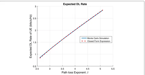
The employment of (24) allows the computation of the rate for the interference limited case in closed form. The tight performance of (24) for the calculation of the ergodic rate is demonstrated in Fig. 3, where (24) is compared against the results obtained by Monte Carlo simulations. Even though the rate does not depend on the density of the

BSs, the density employed for generating the simulation of Fig.3wasλ=1.27e−06.

Several research works have focused on deriving expres-sions for the DL ergodic rate, since the latter constitutes the most sensible figure of merit for evaluating the per-formance of UDNs. Indicatively, in [18] the authors have provided expressions for the DL ergodic rate in heteroge-neous cellular networks for all different types of fading. However, in all of these works, including the latter, the calculation of the DL ergodic rate involved at least one integration that had to be computed numerically. This imposed inherent limitations to the applicability of those expressions to complex optimization problems. In order to overcome this problem, the authors of [19] provided for the first time in the literature expressions for the DL ergodic rate in the interference limited case, for a fully loaded scenario (i.e., forλUEλ) that did not involve any numerical integration. In this direction, the authors of [19] provided lookup tables and employed the Meijer-G func-tion to provide a tight approximafunc-tion of the DL ergodic rate in the fully loaded case. In particular, the approximate ergodic rate of [19] is given by:

C=−s ∗_log

2e 1+s∗

E1

−s∗

Dδ −exp

1+s∗ Dδ E1

1 Dδ

+sin(πδ)log2e π G2,22,3

0, 1−δ 0, 0,−δ

z , (25)

Fig. 3DL ergodic capacity vs path-loss exponent for the interference limited case

all relevant values of β. Furthermore, δ = _β2, D_δ = s∗

log(1−sinc(δ)), En(x) = _∞

1 t−ne−xtdt is the exponential integral and

G_pm_,q,n

a1,. . .,an,an+1,. . .,ap b1,. . .,bm,bm+1,. . .,bq

z =

1 2πi

L

%m

k=1 (s+bk) %n

k=1 (1−ak−s) %p

k=n+1 (s+ak) %q

k=m+1 (1−bk−s) z−sds,

(26)

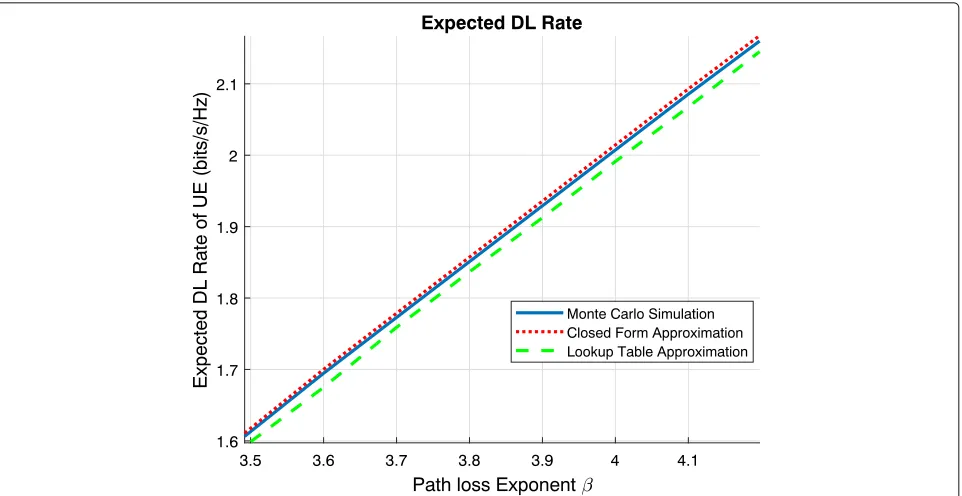
is the Meijer-G function. Improving the result of (25), the present paper introduces for the first time a closed form approximation for the ergodic rate in (24), without the need for an a priori computed lookup table. Furthermore, the result of (24) is significantly more tractable than the result of (25), and Fig.4demonstrates the superior perfor-mance of (24) over (25) with respect to the tightness of the approximation. The accuracy and, more importantly, the tractability of the above expressions allow for the exten-sion of the analysis to even more complex scenarios, as will be demonstrated in the following sections.

5.3 Ergodic rate over density of users and BSs

As already mentioned, the previous analysis corresponds to a scenario where the density of users is much greater than the density of BSs (i.e.,λuser λ) and, therefore, every BS is in transmission mode. However, since in the envisaged UDNs the number of BSs is expected to be higher than the number of UE [9], the analysis needs

to be extended accordingly, taking into account the non transmitting mode of the excess BSs that do not have any UE in their coverage. In this course, the proposed tractable MGF is revised to account for the probability of the excess BSs to remain idle. This probability is defined by the den-sity of UEλUEand the density of BSsλ. Thus, following a similar approach as before, we derive closed form expres-sions for the DL ergodic capacity (i.e., peak and divided among intra-cell users) which depend on the density of UE λUEand the density of BSsλ.

The probability that a randomly chosen BS does not have any UE in its Voronoi cell and, therefore, goes into idle mode is given by [20]:

Pinactive=

1+ λUE 3.5λ

−3.5

(27)

and the probability of a BS being in transmission mode and, thus, acting as an interferer in the DL, is denoted by:

Pactive=1−Pinactive. (28)

Fig. 4DL ergodic capacity vs path-loss exponent for the interference limited case. Tightness of closed form approximation compared to the lookup table approximation employing the Meijer-G function. The range ofβis defined by the range of the respective lookup table provided in [19]

Mg the coverage probability is now given by:

Pcov/active(

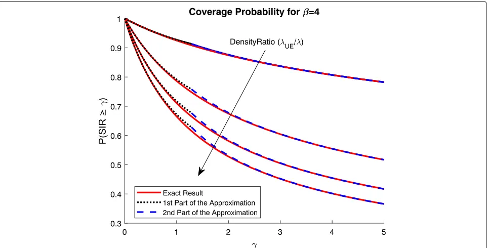
The probability of coverage defined by the exact result of (30a) and by the approximation of (30b) is plotted in Fig.5for a path-loss exponentβ =4 and for density ratios λUE/λ = 0.1, 0.4, 0.7, 1, demonstrating, once again, the accuracy of the derived approximation.

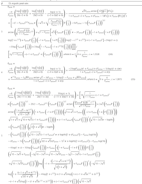
Following the same approach as in (23) for the results of (30b), the DL ergodic peak rate can be computed in closed form as follows:

Rpeak=

For path-loss exponent values ofβ = 3, 4, 5, the closed form expressions for the peak rate are given in Table1. The expressions (34)–(36) provide a closed form representa-tion of the peak DL ergodic rate over the probabilityPactive and, implicitly through (28), over the density of BSsλand of UEλUE.

The probability that a randomly chosen UE is assigned a resource block at a given time and is served by its nearest BS is given by [20]:

Fig. 5Probability of coverage for different density ratios (0.1_{≤λUE/λ≤}1). The density ratio increases in the direction of the arrow with a step of 0.3

resources and, thus, the peak rate among all intra-cell UE. The latter is given by:

R=RpeakPselection. (33)

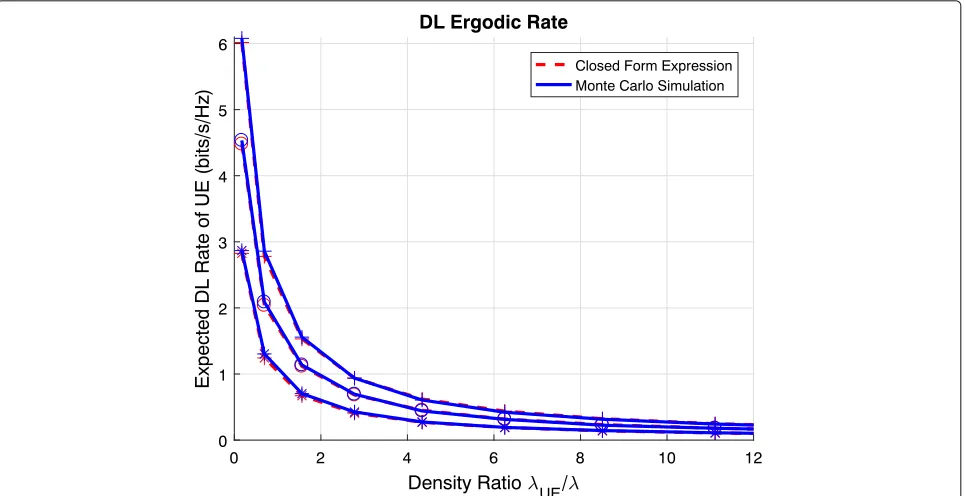
The accuracy of expressions (33)–(36) is demonstrated in Figs.6and7where the peak and the actual DL ergodic rates are plotted over the ratio of the densitiesλUE/λand compared against Monte Carlo simulations.

In the Monte Carlo simulations, the BSs are deployed

following the PPP of density λ and the users are

deployed following the PPP of density λUE, whereas the reference UE resides at the origin. BSs with no UE in their coverage (i.e., within their Voronoi cell) do not create any interference. To compute the actual rate, the num-ber of users residing within the Voronoi cell of BS0 are counted in each realization and the peak rate is divided among these users and the reference UE. The number of simulated BSs is fixed and the simulation area expands or contracts as the BS densityλchanges, in order to accom-modate the predefined number of BSs, while the density of usersλUEremains fixed.

The closed form expressions derived in (33)–(36) pro-vide, among others, a substantial computational gain when compared to the computational time of the respec-tive Monte Carlo simulations. Especially, since the sim-ulation of a wireless network, which comprises both users and BSs of different spatial distributions, and the

calculation of their relative distances, is computationally expensive. In order to demonstrate the gain arising by the employment of the closed form expressions of (33)–(36), the computational time of the derived closed form expres-sions is tabulated in Table 2. Since this time is not an absolute metric, but depends on the hardware employed, Table 2 presents the computational time of the expres-sions as a percentage of the computational time required for simulating the respective wireless networks of Fig.7 using the same hardware.

Table2demonstrates that the computational gain aris-ing by the derived expressions is immense. The time required for the analytical computation of the rate is prac-tically zero compared to the time required for simulating the respective scenario. At this point it should also be noted, that the variations in the values of the computa-tional time arise due to the variations in the time required for the respective simulations. That is since the simulation area has to expand and contract asλchanges in order to accommodate a fixed number of BSs. The variations with respect toβemerge due to the different complexity of the analytical expressions of (34)–(36), with respect toβ.

Table 1Closed form expressions for the DL ergodic peak rate for different path-loss exponents

β DL ergodic peak rate:

3

3Pactivearctan

Table 1Closed form expressions for the DL ergodic peak rate for different path-loss exponents(continued)

β DL ergodic peak rate:

5 log

1+i(−1+ √

5+4c1/5) '

2₍5₊√5₎

−4 log1+c1/5+(1+√5)log2+(−1+√5)c1/5+2c2/5

−(−1+√5)log2−(1+√5)c1/5+2c2/5+

(1+Pactive) ₃

5 2

Pactive

−i ,

2(5+√5)

log

1+i(−1+ √

5₊4c1/5₎ '

2(5+√5)

−4 log1+c1/5−(−1+√5)log2+(−1+√5)c1/5+2c2/5

(1+√5)log2−(1+√5)c1/5+2c2/5+(−1+Pactive) (Pactive)2

3 5

3

i ,

2(5+√5)

log

1+i(−1+ √

5+4c1/5) '

2(5+√5)

−4 log1+c1/5+(−1+√5)log2+(−1+√5)c1/5+2c2/5

+(1+√5)log2−(1+√5)c1/5+2c2/5−2₍−2+P_{active) (}2+Pactive(−2+Pactive))

2 log(1+c)+5 log

Pactive

₃

5

−5 log

1−Pactive+Pactivec2/5

₃

5 *

+10 log

1−Pactive+Pactivec2/5

₃

5 *

/

−4(−1+Pactive)5+4(Pactive)5 ₃

5

5

,

whereb=2 &

16

9 +

2

Pactive

,c=1.3099 (36)

in Section2, that in the fully loaded case (i.e., forλUEλ) the ergodic rate remains invariant while the BS density changes. However, Fig. 7 demonstrates that even if the peak rate remains invariant, the rate of the users that have to share this peak rate tends to zero as the den-sity ratio (i.e., the expected number of users per typical cell) increases. This behavior demonstrates why the envis-aged UDNs are expected to comprise more BSs than

users, highlighting the importance of the non-fully loaded case. Given the importance of the non-fully loaded case, expressions (34)–(36) and Fig.6allow for the first time to quantify the threshold between the non-fully and the fully loaded case. In particular, in all three expressions for the different values ofβ, the network exhibits the behavior of a fully loaded network forλUE/λ > 4, way earlier than implied by the notationλUEλ.

Fig. 7DL ergodic capacity vs ratio of densities_λUE/λfor a path-loss exponent_β=3_(∗), 4₍o₎and 5₍+₎

Another interesting finding can be derived from the behavior of the network in the non-fully loaded case, when the BSs that do not comprise any user in their coverage do not create any interference. In this setup, Fig.6demonstrates that the densification of the network can provide substantial capacity gains, since the achieved DL ergodic rate in this range is significantly higher than the rate achieved at the fully loaded case. Thus, Fig. 6 demonstrates that just by switching off the BSs that do not comprise users in their coverage, substantial capacity gains can be engendered for the network. This motivates the use of even more intricate schemes where BSs can be switched off strategically to mitigate interference. This optimization problem is only one of the problems that the derived expressions can be applied to, with additional applications being presented in the following section.

Moreover, expressions (34)–(36) and the respective figures, verify the results of the expressions (24) and (25), and of Figs.3and4, according to which the DL ergodic

Table 2Computational time of expressions (33)–(36) as a percentage of the respective computational time for simulating the scenarios of Fig.7

Path loss (β) Density ratioλUE/λ

0.17 4.34 8.51 11.11

3 6.9 10−4_{% 6.7 10}−4_{% 3.4 10}−7_{% 2.7 10}−7_%

4 6.9 10−4_{% 6.8 10}−4_{% 1.8 10}−7_{% 1.3 10}−7_%

5 2.2 10−3% 4.6 10−3% 2.3 10−6% 1.6 10−6%

rate increases monotonically with the path-loss exponent β. In particular, since the distance from the UE to the serving BS is always smaller than the distance to the inter-fering BSs, i.e., sincexi > x0, each term of the sum

x∈, x=x0

x0

xi

β

decreases withβ. Consequently, the SIR and

the DL ergodic rate increase monotonically withβ.

5.4 Applications of the derived expressions

Figures 6and7 corroborate the accuracy of the derived expressions, while providing a deeper understanding of the network performance as a function of the user and BS densities. Hence, these expressions, which for the first time associate the DL ergodic rate with the densities of the UE and of the BSs is a closed form, pave the way for the investigation of complex optimization problems, toward improving UDN operation and offered QoS.

In particular, given the maximum density of UE λUE during the operation of the network and the minimum rate requirement per user (imposed by the QoS con-straints), Fig. 7 and (33) can be employed by network operators to define the minimum BS densityλthat guar-antees this rate. Hence, (33) can be employed as a rule of thumb for the lower limit of the densification of BSs that guarantees the QoS objectives, implicitly quantify-ing the minimum capital expenditure required by network operators.

densityλ, comprising UE whose densityλUEvaries during the operation of the network, Fig. 7 and (33) can be employed to dynamically define the probability of trans-missionPactive that achieves the predefined rate require-ment as λUE changes. This probability can indicate the density of transmitting BSs λPactive, i.e., the density of the BSs comprising at least one UE in their coverage. The latter density can be input into optimization mod-ules, to be used as a starting point for the search aiming at pinpointing the optimum set of BSs to be switched off, additionally to those that do not comprise any UE in their coverage. Given the high density of the BSs, strate-gically switching off the best serving BSs of a UE for the latter to be served by a neighboring BS has a only minimal impact on the path loss, while it can provide substantial capacity gains through the mitigation of the interference.

6 Conclusions

The present paper has demonstrated how stochastic geometry tools can be exploited to derive not just exact but cumbersome expressions, but also simple, albeit extremely accurate closed form expressions that allow for the investigation of complex optimization problems. The resolution of these problems is essential in order to reap the capacity benefits of UDNs. In this direction, the present paper presented an accurate and tractable approximation for the MGF of the aggregate other-cell interference. Given the pivotal role of the MGF in stochas-tic geometry analyses, the derived approximation can be employed by a multitude of applications to simplify the analysis and facilitate the derivation of closed form expressions.

Building upon this result, the present paper has focused on the interference limited case, providing very tractable expressions for the coverage probability, as well as closed form expressions for the DL ergodic capacity (i.e., peak and actual) which depend on the density of UEλUEand the density of BSsλ. The derived expressions and their dependence on the user and BS densities set out a den-sification road map for network operators and designers of significant practical and commercial value. Moreover, such expressions can be used for the resolution of com-plex optimization problems in real time, improving the network performance and operation.

Abbreviations

BS: Base station; CCDF: Complementary cumulative distribution function; DL: Downlink; LOS: Line of sight; MC: Macro cell; MGF: Moment generating function; PDF: Probability density function; PGFL: Probability generating fuctional; PPP: Poisson point process; QoS: Quality of service; SINR: Signal to interference plus noise ratio; SIR: Signal to interference ratio; UDN: Ultra dense network; UE: User equipment; UL: Uplink

Authors’ contributions

All authors have contributed to this research work. Moreover, all authors have read and approved the final manuscript.

Funding

The work presented in the present paper has been carried out within the framework of the project ETN-5Gwireless (this project has received funding from the European Union’s Horizon 2020 research and innovation programme under the Marie Skłodowska-Curie grant agreement No. 641985). Moreover, the work has been partially funded through the grant 2017 SGR 578 (funded by the Catalan Government—Secretaria d’Universitats i Recerca, Departament d’Empresa i Coneixement, Generalitat de Catalunya, AGAUR) and the project TEC2016-77148-C2-1-R (AEI/FEDER, UE): 5G&B-RUNNER-UPC (funded by the Agencia Estatal de Investigacion, AEI, and Fondo Europeo de Desarrollo Regional, FEDER).

Availability of data and materials

Not applicable. No datasets were imported or generated while developing the presented material.

Competing interests

The authors declare that they have no competing interests.

Author details

1_{Department of Signal Theory and Communications, Universitat Politècnica}

de Catalunya (UPC), Barcelona, Spain.2_{Laboratoire des Signaux et Systèmes,} CNRS, CentraleSupélec, Univ. Paris-Sud, Universite Paris-Saclay, 91192 Gif-sur-Yvette, France.

Received: 28 January 2019 Accepted: 24 June 2019

References

1. V. Chandrasekhar, J. G. Andrews, A. Gatherer, Femtocell networks: a survey. IEEE Commun. Mag.46(9), 59–67 (2008)

2. F. Baccelli, B. Blaszczyszyn, P. Muhlethaler, An Aloha protocol for multihop mobile wireless networks. IEEE Trans. Inf. Theory.52, 421–436 (2006) 3. M. Haenggi,Stochastic Geometry for Wireless Networks. (Cambridge

University Press, Cambridge, 2013)

4. J. G. Andrews, F. Baccelli, R. K. Ganti, A tractable approach to coverage and rate in cellular networks. IEEE Trans. Commun.59(11), 3122–3134 (2011) 5. H. S. Dhillon, R. K. Ganti, F. Baccelli, J. G. Andrews, Modeling and analysis of

k-tier downlink heterogeneous cellular networks. IEEE J. Sel. Areas Commun.30(3), 550–560 (2012)

6. S. Singh, X. Zhang, J. G. Andrews, Joint rate and SINR coverage analysis for decoupled uplink-downlink biased cell associations in HetNets. IEEE Trans. Wirel. Commun.14(10), 5360–5373 (2015)

7. M. D. Renzo, W. Lu, P. Guan, The intensity matching approach: A tractable stochastic geometry approximation to system-level analysis of cellular networks. IEEE Trans. Wirel. Commun.15(9), 5963–5983 (2016) 8. M. Ding, P. Wang, D. Lopez-Perez, G. Mao, Z. Lin, Performance impact of

los and nlos transmissions in dense cellular networks. IEEE Trans. Wirel. Commun.15(3), 2365–2380 (2016)

9. J. G. Andrews, Seven ways that hetnets are a cellular paradigm shift. IEEE Commun. Mag.51(3), 136–144 (2013)

10. M. Ding, D. Lopez-Perez, G. Mao, Z. Lin, Performance impact of idle mode capability on dense small cell networks. IEEE Trans. Veh. Technol.66(11), 10446–10460 (2017)

11. A. I. Aravanis, O. Munoz, A. Pascual-Iserte, M. Di Renzo, in2019 IEEE 89th Vehicular Technology Conference (VTC2019-Spring), Kuala Lumpur, Malaysia. On the Coordination of Base Stations in Ultra Dense Cellular Networks, (2019), pp. 10–6.https://doi.org/10.1109/VTCSpring.2019.8746531, http://ieeexplore.ieee.org/stamp/stamp.jsp?tp=&arnumber= 8746531&isnumber=8746285

12. S. N. Chiu, D. Stoyan, W. S. Kendall, J. Mecke,Stochastic Geometry and Its Applications. (John Wiley and Sons, West Sussex, 2013)

13. G. Geordie, Device-to-device communication and wearable networks: Harnessing spatial proximity. PhD thesis, Universitat Pompeu Fabra (2017) 14. T. U. Lam-Thanh, New methods for the analysis and optimization of

cellular networks by using stochastic geometry. PhD thesis, Universite Paris-Saclay (2018)

16. J. Lee, F. Baccelli, inIEEE INFOCOM 2018 - IEEE Conference on Computer Communications. On the effect of shadowing correlation on wireless network performance, (2018), pp. 1601–1609

17. S. Sadr, R. S. Adve, Partially-distributed resource allocation in small-cell networks. IEEE Tran. Wirel. Commun.13(12), 6851–6862 (2014) 18. M. D. Renzo, A. Guidotti, G. E. Corazza, Average rate of downlink

heterogeneous cellular networks over generalized fading channels: A stochastic geometry approach. IEEE Trans. Commun.61(7), 3050–3071 (2013)

19. G. Geordie, R. K. Mungara, A. Lozano, M. Haenggi, Ergodic spectral efficiency in MIMO cellular networks. IEEE Trans. Wirel. Commun.16(5), 2835–2849 (2017).https://doi.org/10.1109/TWC.2017.2668414, http://ieeexplore.ieee.org/stamp/stamp.jsp?tp=&arnumber= 7880697&isnumber=7920448

20. S. M. Yu, S. L. Kim, in2013 11th International Symposium and Workshops on Modeling and Optimization in Mobile, Ad Hoc and Wireless Networks (WiOpt). Downlink capacity and base station density in cellular networks, (2013), pp. 119–124.http://ieeexplore.ieee.org.recursos.biblioteca.upc. edu/stamp/stamp.jsp?tp=&arnumber=6576422&isnumber=6576384

Publisher’s Note