Assessing the hazard from geomagnetically induced currents to the entire high voltage power network in Spain

F U L L P A P E R

Open Access

Assessing the hazard from geomagnetically

induced currents to the entire high-voltage

power network in Spain

Joan Miquel Torta

, Santiago Marsal

and Marta Quintana

Abstract

After the good results obtained from an assessment of geomagnetically induced currents (GICs) in a relatively small subset of the Spanish power transmission network, we now present the first attempt to assess vulnerability across the entire Spanish system. At this stage, we have only included the power grid at the voltage level of 400 kV, which contains 173 substations along with their corresponding single or multiple transformers and almost 300

transmission lines; this type of analysis could be extended to include the 220-kV grid, and even the 110-kV lines, if more detailed information becomes available. The geoelectric field that drives the GICs can be derived with the assumption of plane wave geomagnetic variations and a homogeneous or layered conductivity structure. To assess the maximum expected GICs in each transformer as a consequence of extreme geomagnetic storms, a post-event analysis of data from the Ebre Geomagnetic Observatory (EBR) during the 2003 Halloween storm was performed, although other episodes coincident with very abrupt storm onsets, which have proven to be more hazardous at these mid-latitudes, were analyzed as well. Preferred geomagnetic/geoelectric field directions in which the maximum GICs occur are automatically given from the grid model. In addition, EBR digital geomagnetic data were used to infer statistical occurrence probability values and derive the GIC risk at 100-year or 200-year return period scenarios. Comparisons with GIC measurements at one of the transformers allowed us to evaluate the model uncertainties.

Keywords:Geomagnetically induced currents; GIC; Space weather; Natural hazards; Spain

Background

Solar-terrestrial physics is a discipline with a long trad-ition, and many observatories and research groups have been dedicated to this subject for a long time. However, as modern society has become more dependent on techno-logical systems and therefore vulnerable to disturbances in the upper atmosphere and in the interplanetary space near Earth, the focus of this discipline evolved in new and important directions, and it has been renamed as space weather (e.g., Song et al. 2001). Space weather covers the study of the conditions in space that could affect human activity. Phenomena originating in the Sun that can affect human activity include explosive events such as flares and coronal mass ejections. These produce large quantities of

energetic particles and solar wind disturbances, which travel through the interplanetary medium and affect the terrestrial environment. This solar activity is cyclical (solar cycle) and reaches a maximum approximately every 11 years.

The event that sparked global interest in this discipline, beyond academia, was the collapse of the power grid in northeastern Canada due to the great geomagnetic storm of 13 March 1989; this event left millions of people with-out power for 9 h (Bolduc 2002). In October-November 2003, during the declining phase of the next solar cycle, a series of events known as the Halloween storm occurred, and as a result, some new problems in electrical transmis-sion networks were encountered (e.g., there was a black-out in the city of Malmö in sblack-outhern Sweden (Pulkkinen et al. 2005; Wik et al. 2009)) and several space missions and satellites experienced numerous anomalies (Royal Academy of Engineering 2013). Motivated by the events * Correspondence:[email protected]

1

Observatori de l'Ebre, (OE), CSIC, Universitat Ramon Llull, Horta Alta 38, Roquetes 43520, Spain

Full list of author information is available at the end of the article

of 2003, the Committee on Solar and Space Physics (CSSP) of the U.S. National Research Council (NRC) began to consider the need to systematically assess the so-cial and economic impacts of space weather. To establish objectives for this research, the CSSP organized a work-shop in Washington, D.C. during May 2008. The conclu-sions obtained as a result of that meeting can be found in the workshop report (U.S. National Research Council 2008). One of the most obvious conclusions revealed by the historical records is that past space weather events, such as the Carrington event in 1859 (Cliver and Dietrich 2013) and the great geomagnetic storm of May 1921 (Kappenman 2006), have been as much or even more severe than some of the more recent ones; this suggests that such extreme events, although rare, are likely to happen again sometime in the future. As stated in the workshop report, according to a study by the Metatech Corporation, today the occur-rence of an event like the 1921 storm would result in large-scale blackouts affecting over 130 million people and would put more than 350 transformers at risk of perman-ent damage.

Geomagnetic storms caused by disturbances in solar con-ditions can affect the terrestrial environment including the magnetosphere, ionosphere, and magnetosphere-ionosphere interaction region; such effects are detectable at the sur-face of the Earth (e.g., Blanch et al. 2013). The highly con-ductive nature of the ionosphere produces significant current systems in this region, such as the equatorial and auroral electrojets. During disturbed conditions, there is a significant increase in these currents (the auroral electrojet can measure on the order of millions of amps). As these are time-varying, intense induced electric currents appear occasionally in conductors at the Earth's surface. The European Space Agency (ESA) launched the Swarm mis-sion in November 2013 to better understand the magnetic field around Earth. This mission provides opportunities for near real-time in situ monitoring of the ionosphere and upper atmosphere (Stolle et al. 2013).

The induced electric currents generated by geomagnetic storms in ground-based technical networks are called geo-magnetically induced currents (GICs). Their frequencies are typically in the millihertz range, and thus, they can be considered quasi-direct currents (quasi-dc). These currents can disrupt and damage our technological systems, e.g., by affecting transformers of high-voltage networks in the case of power transmission systems. Specifically, transformer cores can saturate under the effect of GICs by operating in the saturation region of the magnetization curve (B-H) of the steel core (Molinski 2002; Kappenman 2007). When a large number of transformers experience GIC saturation, the demand for reactive power and the harmonics of the system voltage are significantly increased. Reactive power demands of this magnitude can cause serious changes in the system voltage. At the same time, the change in the

size of the ferromagnetic material (magnetostriction) be-tween the saturated and unsaturated states at twice the power frequency produces heat, noise, and mechanical vi-bration damage (Koen and Gaunt 2002). The transformers may also suffer premature aging due to the effects of GICs. This aging can be detected by measuring the concentration of gas in the transformer oil. The harmful effects of mag-netic storms on power grids have been observed both at high latitudes and at low and middle latitudes. Damage has even occurred in electrical networks at latitudes lower than Spain, such as in the case of South Africa during the Halloween storm of 2003 (Gaunt and Coetzee 2007). This event was related to the onset of damage in a 700 MVA transformer and in several smaller power transformers. It has been shown (Torta et al. 2012) that during that event, the amplitude of the variations of the horizontal geomag-netic field and its time derivative (dBH/dt), which is more important for geoelectric field generation, were signifi-cantly higher at the Ebre Observatory in Spain than in Hermanus, South Africa. It is therefore prudent that we assess the effects of magnetic storms on the Spanish power network.

Methods

Modeling efforts for calculating GICs in ground-based technological systems require a determination of the elec-tric field that occurs in connection with a magnetic storm at the Earth's surface and a calculation of the resulting GIC (see Pirjola 2002). The practical calculation includes both a geophysical and an engineering problem because the surface geoelectric field is determined from geomag-netic recordings or from ionospheric-magnetospheric current data (if available) as the first step, and then the GIC flow is calculated under the given geoelectric field using the known topology and resistances of a conductor system.

For the determination of the geoelectric field, we have different possibilities. Going from the most sophisticated to the simplest one, one can choose exact formulas for the calculation of magnetic and electric fields at the Earth's sur-face due to an auroral electrojet, which include contribu-tions from field aligned currents (e.g., Pirjola and Häkkinen 1991). However, the resulting formulas are complicated and unsuited to real-time calculations. On the basis of the experience obtained by this study, we attempt to use a practical procedure for the real-time calculation of GICs, which would allow organizations to find the best way of configuring the power system to mitigate their impact as fast as possible.

complex depth. For a source at height h above the Earth's surface, the complex depth is h+ 2p, where pis the complex skin depth related to the surface imped-ance,Z(Wait 1981; Boteler and Pirjola 1998):

pð Þ ¼ω Zð Þω iωμ0

: ð1Þ

Here i, ω, and μ0 are the imaginary unit, the angular

frequency, and the vacuum permeability, respectively. Both the complex skin depth and the surface impedance are defined in the frequency domain. As a first approxi-mation to the auroral electrojet, Boteler and Pirjola (1998) derived algebraic expressions for the magnetic and electric fields at Earth's surface due to an infinite line current above the Earth using CIM. They consid-ered two different conductivity models representative of Québec and British Columbia, which are resistive and conductive, respectively. It has been demonstrated that CIM gives a very good agreement with the exact meth-odology. Although it is a convenient tool for theoretical modeling purposes, it is not the most optimal choice for more operational applications because it was simply de-rived for a line current above the Earth. However, Pirjola and Viljanen (1991) show that the applicability of CIM is not restricted to the line current case as they extended the use of CIM to a more complicated ionospheric-magnetospheric current system. Pirjola et al. (2000) also show the successful use of CIM for a westward-traveling-surge (WTS) event.

Since the true 3-D ionospheric current system cannot be determined by using ground magnetometer data only, the method of Spherical Elementary Current Systems (SECS) (Amm 1997) can be used to introduce a horizon-tal equivalent current system, which produces the same magnetic and electric field at the Earth's surface. This method is based on the fact that geomagnetic variations at the Earth's surface can be explained by a horizontal divergence-free current system at the ionospheric level. The amplitudes of the elementary current systems are determined by the inversion technique, by fitting the modeled horizontal field to the measured one, and once the currents are determined, obtaining the electric field at the Earth's surface due to one element is straightfor-ward. Inversion is usually resolved by the singular value decomposition technique because the system is typically underdetermined. Data for just three magnetic observa-tories have even been reported to have been used in the interpolation process to infer the equivalent ionospheric currents (Caraballo et al. 2013).

The CIM and the SECS technique are commonly used to determine the geoelectric field at high geomagnetic latitudes. Pulkkinen et al. (2003) presented a calculation using a combination of both techniques. At mid-latitude

regions, however, the source field is rather uniform, and if we happen to have geomagnetic field variations mea-sured sufficiently close to the location where the GIC is computed, a simple and practical way to estimate it is to assume a downward-propagating plane wave impinging on either a uniform or a layered Earth. In this plane wave model, the electric and magnetic fields are hori-zontal and spatially constant at the Earth's surface. If, in addition, the Earth is uniform, a time-domain integral relation can be obtained, which easily allows for the use of magnetic observatory data to derive the GIC (e.g., Pirjola 2002; Ngwira et al. 2011; Torta et al. 2012). Note that in Ngwira et al. (2011) and Torta et al. (2012), the derivative of B must be with respect to u rather than with respect tot:

where x and y indicate the north and east geographical directions, respectively; μ0 is the permeability of free

space; and σ is the Earth's conductivity. The‘+’sign on the right-hand side applies to (Ex, By) and the‘−’sign to

(Ey, Bx). In contrast, if one considers a layered Earth

structure, the surface impedance Z(ω) can be obtained

for each angular frequencyωby a recursive formula that determines the impedance at the top of any layer in terms of the impedance at the bottom of the layer (see, e.g., Pulkkinen 2003). The geoelectric field in the time domain is then evaluated by the inverse Fourier trans-form of

Ex;yð Þ ¼ ω Zð Þω_μBy;xð Þω

0

; ð3Þ

where B(ω) is the Fourier transform of the magnetic

field (e.g., Viljanen et al.2006). The integral in Equation2

can be easily obtained numerically (Viljanen and Pirjola

1989). In evaluating that integral in practice, the lower limit of integration of Equation2is set tot-M, whereM

is the amount of time taken into account before t (for which the electric field is required). If this interval is suf-ficient, the time-dependent method (valid for a uniform Earth) provides the same results as the spectral method (valid for the layered Earth) provided that all the layers are given the same conductivity.

Matrix (MIM) method or the Nodal Admittance Matrix (NAM) method, which are used by the power industry (e.g., Albertson 1989), or the Lehtinen-Pirjola (LP) method (Lehtinen and Pirjola 1985), which has been used trad-itionally by the geophysics community. Actually, NAM and LP are the same, with the exception that NAM cannot deal with the interaction between the nodes described by the off-diagonal elements of the earthing impedance matrix in LP (see next paragraphs). The calculation tech-nique in the MIM method is different but equivalent with NAM and LP in the sense that it is also based on circuit analysis and Ohm's and Kirchhoff's laws (R. Pirjola, per-sonal communication). Following with that tradition, we used the LP method as well. Knowing that GICs are slowly varying compared to the 50-Hz mains, a dc treatment is acceptable, and so we simply used Ohm's and Kirchhoff's laws in the dc form to formulate a network matrix model from the earthing/transmission line resistances provided by industry data. Lehtinen and Pirjola (1985) provided all the expressions that lead to the determination of the GIC (I) flowing into the Earth (or into the grid) at each of then nodes. They can be summarized in the following equation:

I¼ð1þYZÞ−1J; ð4Þ

where 1,Y, andZ are the identity matrix, the nxn net-work admittance (related with the line resistances) matrix, and the earthing impedance (related with the earthing resistances) matrix, respectively; the n-element vector J contains information on the electric field com-puted, as described before, from geomagnetic observa-tory data.

The elements of theY and Z matrices are computed according to (Lehtinen and Pirjola 1985)

Yij¼

where Rij is the line resistance between nodes i and j,

and if the nodes are far apart,

Zij¼ 0; i≠j

Rei; i¼j ;

ð6Þ

where Rie is the resistance through which the node i is

earthed. Pirjola (2008a,b) demonstrated that accounting for the off-diagonal elements of this matrix can be only relevant when the distances between the stations are on the order of hundreds of meters or less. In the Spanish 400-kV network described in the next section, only three node links are separated by less than 500 m (between approximately 350 and 450 m), so all the off-diagonal el-ements of the earthing impedance matrix were set equal to zero. In any case, neglecting all off-diagonal elements

of Z is in general less important for the knowledge of the expected GICs than the uncertainties produced by the different approximations and assumptions adopted because it is not always possible to get precise values for all the circuit elements.

TheJvector in Equation 4 is given by

Ji¼

whereVijis the geovoltage from nodeito nodej, which

is given by

Vij¼ Z

Lij

E⋅dl; ð8Þ

where Eis the electric field, dlis the differential vector path length, and the integration path Lij refers to the

transmission line fromitoj. IfEis conservative, the in-tegral in Equation8is independent of the pathLijfromi

to j, andVij=Vi−Vj, where Vi and Vj are the values of

the scalar potential of the geoelectric field at nodesiand

j. A particular case of a conservative field is when it can be considered spatially constant in the region of analysis. Then, the GIC values in each node can be expressed in terms of two parameters (aandb), which depend on the geometry and the resistances of the network (and natur-ally vary from node to node):

GICð Þ ¼t aExð Þ þt bEyð Þt : ð9Þ

In summary, the external (or geophysical) conditions are contained in (Ex,Ey), while the engineering problem is determined by the scalar constants a and b. Unless one evaluates continental regions (Viljanen et al. 2012), the Earth's curvature can be neglected and planar geom-etry (rather than spherical) can be used to derive these constants. Horton et al. (2012) even consider the fact that the Earth is not exactly a sphere but an ellipsoid (utilized in global positioning system (GPS) applications that power companies also use).

Results and discussion Data and results

model, with the exception of Mellousa (the second in Morocco) because the first one (Fardioua) is a station without transformers. This is a common practice (e.g., Myllys et al. 2014) because it has been shown (Boteler et al. 2013) that the best choice for an equivalent circuit of the neighboring network comprises the induced volt-age and resistance for the first transmission line into the neighboring system, so that it can be represented as the line to the first substation and its resistance to ground.

Information relating to the resistances of all the trans-formers is still incomplete, so that, for simplification, we

completely ignored the autotransformers' low-voltage circuits, whereby the winding resistance is the sum of the common and the series resistances. For calculating the total earthing resistance at each substation, we con-sidered the three phases in parallel and added the sub-station earthing resistance to their equivalent resistance. If the substation is composed of more than one trans-former, we assumed that the transformers are connected in parallel and share the same substation earthing resist-ance. The values of these earthing resistances are in gen-eral unknown, but we assumed that they have a typical

−500 −400 −300 −200 −100 0 100 200 300 400 500

value of 0.15 Ω (private communication with related power engineers), except for those few substations of the Catalan subset for which we obtained a different value from our previous project. Similarly, in the cases where the resistance of the windings of transformers is un-known, following the criterion of Viljanen et al. (2012), we assumed thatRietakes a typical value of 0.5Ω, which implies a total resistance for three parallel windings of 0.35 Ω, or 1.05 Ω for one winding. The phase resis-tances of the power transmission links were calculated according to the values of the resistance per unit length of the conductors at 20°C and the number of conductors per phase supplied by the power company. Then, one must take into account the reduction of three phases into a single conductor.

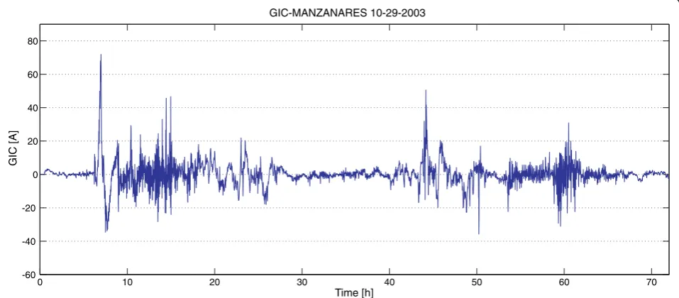
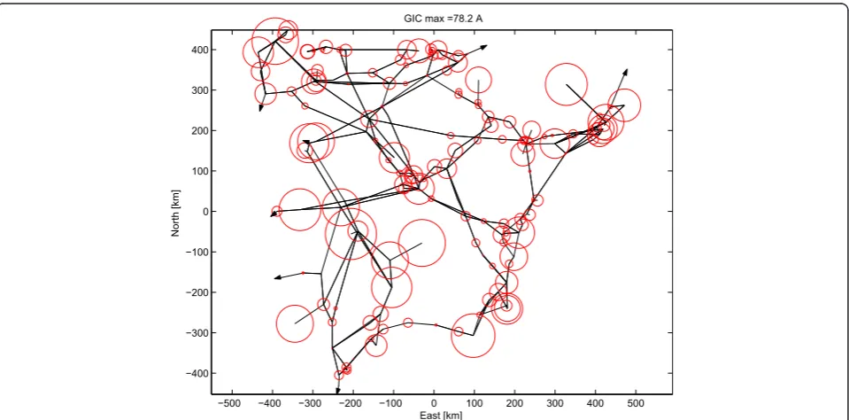
As described in the previous section, theYandZ matri-ces computed from the above resistance data allow for the GIC computation at each substation. Accordingly, we ob-tained a prediction (retrospective in this case) of the GICs in the network nodes and transformers for the Halloween storm and the 24 March 1991 storm, which displayed the most abrupt solar storm commencement at the Ebre Ob-servatory (Torta et al. 2012). We assumed the current net-work configuration and all elements in operation. Figures 2 and 3 show the resulting GIC in the transformer that we identified as the most vulnerable because it was isolated at the end of a line. On occasion of the abovementioned events, in this transformer, we computed 70 and more than 100 A, respectively. In fact, GICs have been calculated as functions of time through the entire Halloween storm of 29 to 31 October 2003, and the maximum absolute value for each individual substation has been taken and plotted in the map of Figure 4 as circles with diameter

proportional to the absolute value of the current. This means that the maxima shown in Figure 4 were not ne-cessarily obtained at the same time point. Large GICs were found in the stations located at the end, or in the corners of transmission lines as intuitively expected and shown by the explicit model calculations for the GIC (e.g., Viljanen and Pirjola 1994; Wik et al. 2008).

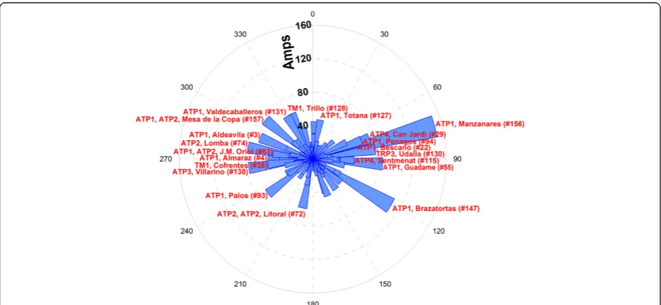
In order to analyze in a more generic way how the differ-ent directions of the electric field affect the GICs generated in the network, we applied a synthetic electric field of modulus equal to 1 V/km in all directions. This value is slightly higher than the maximum value in the geomag-netic records of the Ebre Observatory (i.e., 0.73 V/km, which occurred during the storm of 24 March 1991), but it is a reasonable value for a particularly severe geomagnetic storm scenario and can always easily be scaled to corres-pond to any other uniform-field value (Pirjola 2008a). The obtained results are shown in Figure 5, and these represent those directions in which the maximum GIC flowing from the network to the Earth is reached at each node. The north corresponds to an angle of 0° and the east to an angle of 90°. The length of the vectors indicates the max-imum magnitude, and one must take into account that it is reached both in the given direction and in the opposite direction because a field reversal only changes the signs of the GICs (see Equation 9). In any case, as indicated by Bernabeu (2013), their impact on driving transformers into half-cycle saturation is independent of the direction of the current flow. Only those nodes that would achieve signifi-cant currents have been labeled (with the name of the sub-station and an indication of the number ascribed to them in Figure 1). From Figure 5, it can be deduced that the maximum GICs are achieved for those events in which the

0 10 20 30 40 50 60 70

-60 -40 -20 0 20 40 60 80

GIC-MANZANARES 10-29-2003

GIC [A]

Time [h]

electric field direction coincides with the directions of the transmission lines. Given the geometry of the Spanish net-work, these directions are mostly NW-SE and ENE-WSW, and attention should be drawn to the magnitude of the GICs reached at Muruarte and Litoral substations, espe-cially at the latter when the field is in the NNE-SSW direc-tion. In the same way, Figure 6 was obtained by dividing

the GIC values shown in Figure 5 among the transformers of each substation according to the corresponding current divider (i.e., in a ratio depending on the transformer resis-tances). Looking only at the total GIC value at a substation sometimes gives a good idea of the possible GIC hazard, which was the case, for example, at Manzanares (node 156 in Figure 1) and Brazatortas (node 147), which had just

0 10 20 30 40 50 60 70

-100 -80 -60 -40 -20 0 20 40

GIC-MANZANARES 03-24-1991

GIC [A]

Time [h]

Figure 3Geomagnetically induced currents during the magnetic storm on 24 to 26 March 1991.The GICs were calculated in the neutral point of the only transformer at the Manzanares substation (node 156).

one transformer. However, this practice sometimes overes-timated the possible GIC hazard, which was the case at Litoral and Puentes G. R., which had several transformers.

Just as in the previous paragraph, in Figures 7 and 8, we show how GICs affect the Spanish network under the im-pact of a northward (Figure 7) and eastward (Figure 8) geoelectric field of 1 V/km. This value does not accurately

represent the real situation, as the field is never homoge-neous; it varies both due to spatial variations of the ex-ternal geomagnetic field (especially, depending on the latitude) and due to spatial variations of the field created by currents induced in the crust and upper mantle (be-cause of the remarkable heterogeneity in Earth's conduct-ivity). But it is a reasonable magnitude for an extreme

Figure 5Directions in which the maximum GIC is obtained in each node.They correspond to GICs from the network to the Earth when a horizontal electric field of 1 V/km is applied. The length of each bar indicates the maximum current.

−500 −400 −300 −200 −100 0 100 200 300 400 500 −400

−300 −200 −100 0 100 200 300 400

E = 1 V/km North, GIC max =153.12 A

East [km]

North [km]

100 A

Figure 7Maximum GICs due to a horizontal geoelectric field of 1 V/km in the northern direction.Data are shown in the form of circles, and the diameters are proportional to the flowing current. The red color denotes GICs flowing into Earth, and blue denotes those flowing into the grid.

−500 −400 −300 −200 −100 0 100 200 300 400 500 −400

−300 −200 −100 0 100 200 300 400

E = 1 V/km East, GIC max =146.07 A

East [km]

North [km]

100 A

geomagnetic storm at the latitudes of interest of this study, and that selection is actually unimportant for the purpose of analyzing the vulnerability of the network because, as pointed out above, the values of the GICs are scaled pro-portionally to the electric field (Pirjola 2008a).

Clearly, in a real situation, the geomagnetic field varies in any direction and, consequently, so does the geoelec-tric field. Thus, the generated GICs will be variable but in proportion to the amplitudes shown in Figures 7 and 8. What is unchanged is the realization, as indicated by Boteler (1994) and Pirjola (2008b), that the GICs are maximized when the incident electric field is in the dir-ection of the bisector of the angle formed by two trans-mission lines arriving at a substation and minimized in the perpendicular direction. Thus, the transformers at intermediate stations along a long line are not particu-larly vulnerable to GICs, and therefore, in principle, they are not interesting sites to undertake measurements.

The next step was the estimation of the return period of a hypothetical extreme event. We relied on the results of Thomson et al. (2011), who, using a number of de-cades of 1-min mean data, provided the maximum values observed in the derivative for both the horizontal intensity and the declination of the magnetic field and the values that could be observed every 100 or 200 years depending on the geomagnetic latitude of different European geomagnetic observatories; these data were presented along with the confidence limits at the 95% level. For their analysis, they used a Generalized Pareto Distribution (GPD) to describe the tail of the distribu-tion of geomagnetic activity. Before fitting each GPD to the data, they discarded data located below a certain threshold and isolated the magnetic field of external ori-gin by subtracting the average level on a quiet day (set for each month of the year), thereby obtaining the re-sidual intensityBH and declinationBD. Meanwhile, they grouped extreme events that were less than 12 h apart (taking the maximum value for the period) on the grounds that they were part of the same geomagnetic storm event. For each observatory, they computed the peak residual and peak rate-of-change predicted by the observatory GPD to be exceeded within the periods of 100 and 200 years, which was accomplished via the examination of the return-level statistics. The results of

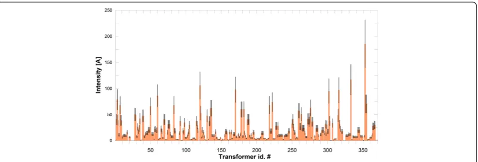
Thomson et al. (2011) appear excessively high for the Ebre Observatory compared with those from observator-ies of similar geomagnetic latitude. This may have hap-pened because the data used still contained artificial peaks in 2001. The predictions made by Thomson et al. (2011) were recalculated after we provided them with geomagnetic data that were reviewed for the period 2000 to 2010 (Table 1); this reanalysis yielded an ex-treme value of 308 nT/min fordBH/dtduring the return period of 100 years. This value was used to obtain an ap-proximate size of the GIC magnitudes that would flow in each of the transformers of the grid in the event that the extreme value actually occurred during the return period of 100 years at the Ebre Observatory, and we as-sumed an impulsive event at a cadence of 1 min along the geomagnetic North (Figure 9). As indicated by Torta et al. (2012), the northward impulse is the most plausible scenario for the most severe events at Ebre Observatory's latitude, where they tend to occur coinci-dent with the abrupt onset of geomagnetic storms.

Errors by the omission of low-voltage circuits

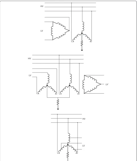
Although it is a common practice to treat the highest-voltage system as the first approximation, as we did in this study, the correcting terms needed to match the ac-tual flowing currents in the interconnecting transformers will not be attainable until we get the necessary data as-sociated with the lower-voltage systems. To illustrate the amount of error that can be expected by the omission of low-voltage circuits of the network, we used data from a test case that was released to validate the programs and procedures used by the scientific and technical commu-nity to model the GICs (Horton et al. 2012). Such a benchmark network contains many features found in real networks, such as different voltage levels, two- and three-winding transformers, autotransformers, multiple transmission lines in the same bus, and GIC-blocking devices (see Figure 10 for simplified expressions of the different resistance structures of transformers). It repre-sents a hypothetical 20 bus network with 8 substations, including 15 transmission lines and transformers of 500 and 345 kV. To model the GICs, Horton et al. (2012) provide three sets of necessary resistance data, i.e., data for the substations, transmission lines, and transformers.

Table 1 The measured maximum and estimated 100-year and 200-year return levels at the Ebre Observatory

Variable Measured maximum 100-year return level Confidence limit 200-year return level Confidence limit

BH 552 706 511 1,358 770 534 1,509

dBH/dt 112 308 231 384 428 320 535

BD 0.87 1.42 0.81 2.59 1.67 0.85 3.09

dBD/dt 0.15 0.25 0.18 0.33 0.31 0.22 0.40

For the residual horizontal intensityBH(in nT), the residual declinationBD(in degrees), and their derivatives (in nT/min and degrees/min, respectively); data are

They also provide geographical positions of the substa-tions (from which one can calculate distances between them in kilometers).

Horton et al. (2012) provide the calculated GIC results in the network for two geoelectric field scenarios: again, a northward and an eastward uniform electric field of 1 V/km. It was found that we could obtain the same re-sults with our programs. To achieve this, in the case of autotransformers, we had to make use of the concept of virtual nodes (Mäkinen 1993; Pirjola 2005) with an infin-ite resistance to ground and a resistance of a virtual line between the virtual and the real node equal to the series resistance of the actual autotransformer, while the com-mon resistance is the resistance of the real transformer at the neutral point. Similarly, for full-wound trans-formers with a Y configuration and grounded both at high- and low-voltage sides, we used an equivalent cir-cuit with two virtual nodes, one in each side of the transformer. Here, again, the virtual nodes have infinite resistances to ground and the virtual line resistances have been set between the virtual and real nodes equal to the real resistances of the transformer windings. Meanwhile, the actual transformer winding resistance was set to zero because it was located at the neutral point of the full-wound transformer.

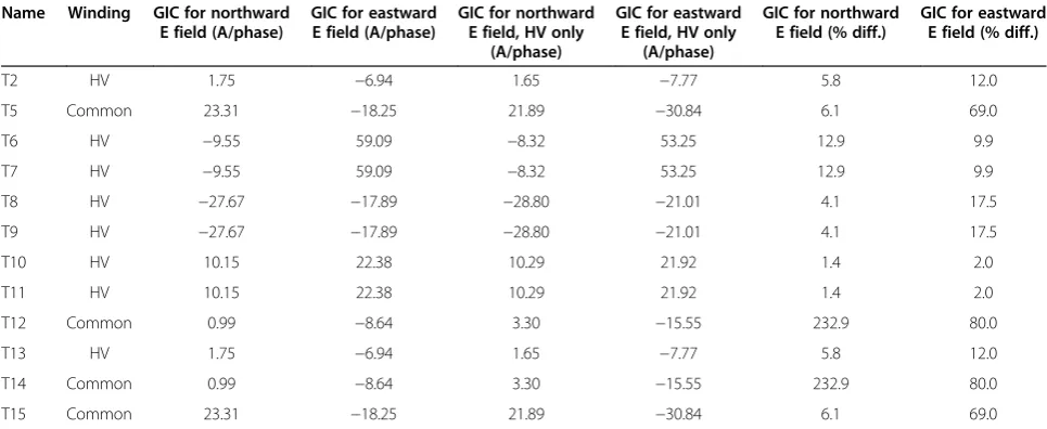
We performed test calculations by omitting the entire low-voltage circuit (345 kV in that case). The results for the GICs flowing to ground at each substation are shown in the two central columns after the column of names in Table 2, whereas those flowing in the phases of each of the transformer windings are shown in the same columns of Table 3. In both tables, the values obtained by Horton et al. (2012) when both the high and the low voltage are considered are also shown (first two col-umns), along with the percentage differences with re-spect to our test (last two columns). It is both clear and

logical that the largest differences were obtained in sub-stations that share lines of high and low voltage. The substations with autotransformers had the largest error (more than 200% in some cases depending on the di-rection of the incident electric field), and at these loca-tions, the GICs were usually overestimated when only the high-voltage circuit was modeled. The corrections of calculated GICs in the Spanish 400-kV network that are needed to account for the effects of neglecting the lower-voltage systems might be different. In any case, this test highlights the importance of having all the in-formation concerning the positions and resistances of the network and the substation configurations, both for the high-voltage circuits and for the low-voltage ones, especially if there is galvanic connection between them.

Comparisons with GIC measurements

The best way to evaluate the performance of a model such as the one described here is to compare its predic-tions at a particular transformer neutral point with ac-tual GIC measurements. This, although planned, is still not possible at key sites such as the transformer at the Manzanares substation. The only measurements coinci-dent with relevant geomagnetic storms were those ob-tained in 2011 to 2012 on behalf of our previous project (Torta et al. 2012). We do compare here the real obser-vations with the predictions of our new model, including the entire 400-kV Spanish network, for the same trans-former named TRP1 (which was wrongly named as TR2 in Torta et al. 2012) at the Vandellòs substation (node 132 in Figure 1) on the occasion of the geomagnetic storm which occurred during 24 to 25 October 2011. Fortunately, there are no autotransformers in this sub-station, so it is not galvanically interconnected with low-voltage systems and thus we do not expect major errors by ignoring the 220- or 110-kV networks at

HV

LV

HV

LV

LV’

HV

LV

farther 400-kV stations (Pirjola and Viljanen 1991; Viljanen and Pirjola 1994; Pirjola 2005, 2010).

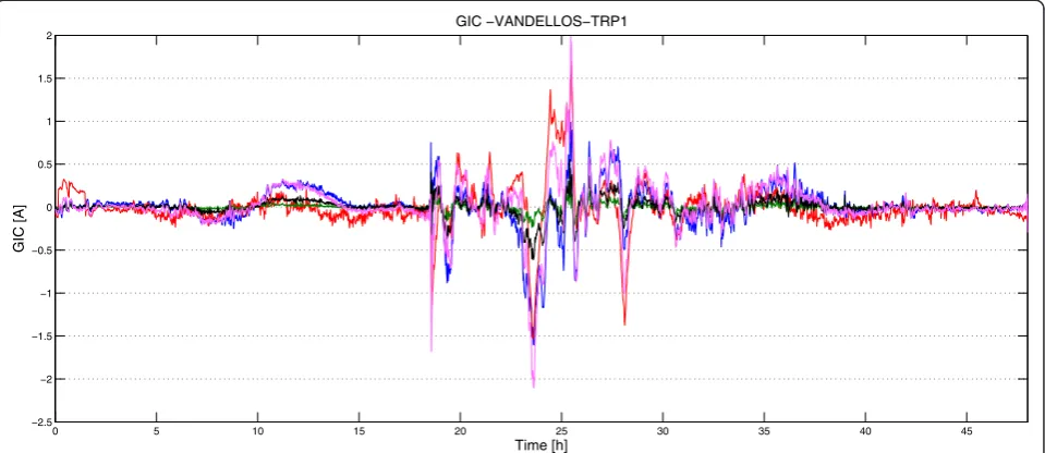
In Figure 11, we show the performance of our model as a function of the Earth conductivity structure that we used. We practiced either with a uniform ground con-ductivity of σ= 0.001 S/m (as in Torta et al. 2012) or with different layered conductivity models. For the latter, we chose either the electrical resistivity model given by Pous et al. (1995) for the Ebre basin or the 1-D ground model of the #29 block in Figure 2 by Viljanen et al. (2012). In Table 4, we give the linear correlation coeffi-cients for each case, but in our opinion, this measure is not always the best indicator for quantifying the good-ness of such model performances. This is because models that provide the same signal but are amplified several times will provide the same correlation coeffi-cients. Thus, to evaluate how well the model fits the

GIC observations, we define the performance (P) param-eter as

P¼1−RMSDom

σo ; ð

10Þ

whereσo is the standard deviation of the set of

observa-tions and RMSDomis the root mean square deviation of

the residuals (or differences between model predictions and observations). Here, the

RMSDom¼

ffiffiffiffiffiffiffiffiffiffiffiffiffiffiffiffiffiffiffiffiffiffiffiffiffiffiffiffiffiffi X_N

i¼1ðoi−miÞ 2

N

s

; ð11Þ

whereoi and miare the ith observation and model

out-put, respectively (or equivalently, those corresponding to time ti), from a total of N. Given that the quotient in

Equation10is a positively defined quantity,Pcannot be Table 2 Comparison of the total GICs flowing in the ground grid of each substation

Name GIC for northward E

field (A)

GIC for eastward E field (A)

GIC for northward E field, HV only (A)

GIC for eastward E field, HV only (A)

GIC for northward E field (% diff.)

GIC for eastward E field (% diff.)

Sub 3 139.85 −109.49 131.33 −185.03 6.1 69.0

Sub 4 19.98 −124.58 29.66 −139.94 48.4 12.3

Sub 5 −279.08 −65.46 −172.81 −126.07 38.1 92.6

Sub 6 −57.29 354.52 −49.92 319.51 12.9 9.9

Sub 7 0.00 0.00 0.00 0.00 0.0 0.0

Sub 8 60.90 134.30 61.74 131.53 1.4 2.1

The table shows the comparison of the total GICs flowing in the ground grid of each substation for the benchmark test case (Table VII of Horton et al.2012) when a northward or eastward uniform electric field of 1 V/km was present (first two columns after the column of names), and the GICs obtained using only the high-voltage circuit. The percent differences (% diff.) data are also shown. HV stands for high voltage.

Table 3 Comparison of the total GICs flowing in the transformer windings

Name Winding GIC for northward

E field (A/phase)

GIC for eastward E field (A/phase)

GIC for northward E field, HV only

(A/phase)

GIC for eastward E field, HV only

(A/phase)

GIC for northward E field (% diff.)

GIC for eastward E field (% diff.)

T2 HV 1.75 ₋6.94 1.65 ₋7.77 5.8 12.0

T5 Common 23.31 ₋18.25 21.89 ₋30.84 6.1 69.0

T6 HV ₋9.55 59.09 ₋8.32 53.25 12.9 9.9

T7 HV ₋9.55 59.09 ₋8.32 53.25 12.9 9.9

T8 HV −27.67 −17.89 −28.80 −21.01 4.1 17.5

T9 HV −27.67 −17.89 −28.80 −21.01 4.1 17.5

T10 HV 10.15 22.38 10.29 21.92 1.4 2.0

T11 HV 10.15 22.38 10.29 21.92 1.4 2.0

T12 Common 0.99 −8.64 3.30 −15.55 232.9 80.0

T13 HV 1.75 −6.94 1.65 −7.77 5.8 12.0

T14 Common 0.99 −8.64 3.30 −15.55 232.9 80.0

T15 Common 23.31 −18.25 21.89 −30.84 6.1 69.0

greater than 1, which is reached when the residuals are zero, i.e., when the model exactly fits the observations. Otherwise, P< 1. P would be 0, for example, for a flat model output equal to the mean of the observations. A negative value of P usually (though not necessarily) de-notes anti-correlation. So, in summary, models that per-form better have higher values ofP, and one can think of

P(with some reservations) as the fraction of the standard deviation of the observations that can be explained by the model. Results for this parameter are also given in Table4

for each of the conductivity case structures tested. None of the proposed 1-D conductivity structures performed substantially better than the homogenous Earth approach, which suggests, as expected, that the actual structure must be laterally heterogeneous, especially because the lateral conductivity contrast is large at ocean-land interfaces (Beggan et al. 2013; Püthe and Kuvshinov 2013); this

makes the 1-D assumption probably invalid in the coastal area.

Since the calculated GIC at one site is slightly sensitive to changes made at distant points of the network (Pirjola 2009), our results can be reasonably compared with those presented in Figure 6 by Torta et al. (2012), when only a subset of the grid was modeled. It is well known that the load and operating procedure of the grid change over time. When we prepared our previous model, we did not have the exact elements of maintenance condi-tions (switched off ) for the occasion of the geomagnetic storm, so we had to resort to the state of the grid that happened on a particular day about 3 months later, in which the lines Ascó (node 13 in Figure 1)-Pierola (node 98), Vandellòs (node 132)-Pierola (node 98), and Vandellòs (node 132)-Rubí (node 107) were switched off. Now,Red Eléctrica de Españahas provided us with updates regard-ing the elements of maintenance durregard-ing 24 to 25 October 2011. The first important realization was that, on that oc-casion, one of the transformers at Vandellòs was switched off so that the total current produced by the geomagnetic storm could not be shared among the two transformers at that substation; hence, it only flew through the neutral point of the TRP1 transformer. This explains why the pre-dictions of Torta et al. (2012) were underestimated and they had to artificially decrease the ground conductivity to match the amplitudes of measured and modeled GICs. However, although the overall amplitudes of the present study agree with more realistic conductivity values, our present results correlate worse with the measures of Torta et al. (2012). There are two explanations for this. The first

0 5 10 15 20 25 30 35 40 45

−2.5 −2 −1.5 −1 −0.5 0 0.5 1 1.5 2

GIC −VANDELLOS−TRP1

GIC [A]

Time [h]

Figure 11Measured and calculated GIC at the TRP1 transformer in Vandellòs.They correspond to the event on 24 to 25 October 2011. The measured GIC is in red. The results are from analyses that used either a uniform ground conductivity set to 0.001 S/m (blue), a layered

conductivity structure according to Pous et al. (1995) (green), a layered conductivity structure according to Viljanen et al. (2012) (black), or a uniform ground conductivity under the condition where the Vandellòs-Pierola transmission line was switched off (pink).

Table 4 Quantification of the goodness of different model predictions

Earth conductivity structure _{ρ P}

Uniform 0.372 0.051

Layered (Pous et al.1995) 0.368 0.045

Layered (Viljanen et al.2012) 0.377 0.074

Uniform (under the condition where the Vandellòs-Pierola line was switched off)

0.749 0.252

one lies in the fact that Torta et al. (2012) used the time-domain integral approach to infer the electric field from the geomagnetic variation data by settingM equal to just 30 min. This converted the data into a surprising result because one would expect that the spectral method or the time-domain method with a sufficiently high M should give a better fit for the GIC data (in this study, we used values ofMaround 300 min, which yielded results similar to the spectral method). UsingM= 30 means that Torta et al. (2012) truncated the impulse response to include only fast variations (i.e., high frequencies). This, in com-bination with the Earth model that is perhaps not exactly correct, happened to lead to a good fit with measured GIC data (R. Pirjola, D. Boteler, personal communication). A second explanation is related to the topology of the grid in the vicinity of the measuring substation. Besides the sec-ond transformer at Vandellòs, the switched off elements in the present model just included the Vandellòs-Rubí trans-mission line (other switched off elements far apart are not prone to influence the currents at Vandellòs). If we omit again the Vandellòs-Pierola line, the correlation signifi-cantly improves (Table 4, last row). We suspect that, al-though not reported, this transmission line or the Vandellòs-Garraf (node 51 of Figure 1) line, which runs al-most parallel, was not operating for at least some time during the storm.

Conclusions

There is no doubt that space weather effects are an emerging natural hazard, which can have incredibly im-portant effects on our lives, which are marked by in-creasing levels of technological dependence. They are in the category of high-impact, low-frequency event risks. When space weather effects refer to induced currents in technological systems such as power transmission grids, they are called geomagnetically induced currents, or simply, GICs. Modeling efforts require a determination of the electric field occurring in connection with a mag-netic storm at the Earth's surface. There are several pos-sible ways to accomplish this task. Once the geoelectric field is obtained, one can calculate the resulting GIC in the conductor system after obtaining a dc model of it. This engineering task requires knowledge of the geomet-rical configuration of the network stations and their con-nections, and also the resistance values of the whole system.

This paper provides much useful information about the expected GIC values in the entire Spanish 400-kV power transmission network, which enables us to con-duct an assessment of the vulnerability from that hazard. The network contains 165 substations, to which we added 8 substations from France, Portugal, and Morocco across the respective borders. This represents a complex circuit with 375 transformers and 300 transmission lines.

After obtaining the electrical network model to evaluate the maximum expected GIC in each transformer as a re-sult of extreme geomagnetic storms, we developed a post-event analysis from the geomagnetic data obtained at the Ebre Observatory during certain storms, such as the Halloween storm in 2003. We also analyzed other episodes coincident with very abrupt sudden storm com-mencements, as they have proven to be even more dan-gerous in mid-latitudes. We found, as expected, that the most susceptible substations to GICs are those in cor-ners or edges of the network. A typical case is that of the Manzanares station which, by having a single trans-former, makes it particularly vulnerable. Had the storm of 24 March 1991 occurred with the current network configuration and with all the elements operative, GICs would exceed 100 A in the neutral point of the trans-former. However, this extreme value will surely be sig-nificantly reduced when transmission lines that are under construction join Manzanares with another sta-tion to the east and become operasta-tional.

Assessing the vulnerability of a system to GIC hazards usually does not require knowledge of the precise values of expected GICs, instead rough magnitude estimates are sufficient (Pirjola 2008a). However, substantial improve-ments in our enterprise could be attained with further insights. A clear source of uncertainty in the obtained re-sults arises from the fact of having completely ignored the low-voltage circuits that are galvanically connected to the 400-kV system through autotransformers. This was done because we had neither information on the 220 kV net-work nor the separate value of the common and series winding resistances of these autotransformers. The 110-kV grid obviously does not have a very big effect on the GIC in the 400-kV system since the lower the voltage, the higher the transmission line resistances, which makes the GICs smaller. The importance of the omission of the low-voltage network has been demonstrated through a test under a GIC benchmark network that has been re-cently developed by Horton et al. (2012).

the specific value of proportionality between the GIC and the electric field only as an‘effective conductivity’(Viljanen 1998). Therefore, another improvement would be expected after realistically modeling the induced electric field on the surface of the Earth by using a 3-D model of Earth's con-ductivity, and this can be done in the manner of recent works such as those by Beggan et al. (2013), Dong et al. (2013), and Püthe and Kuvshinov (2013). In particular, Spain is located on a peninsula, so a precise estimation of the geoelectric field would benefit from modeling the ef-fects of non-uniform conductivities produced by the coast (Gilbert 2005; Thomson et al. 2005; Bürstinghaus et al. 2013; Pirjola 2013).

A critical fact, nevertheless, is the difficulty of obtaining detailed network parameters in the precise instant of a geomagnetic storm and determining the topology of the network for a given amplitude of the incident field. The switching off of a key transmission line or transformer can be essential to boost significant currents through the remaining elements.

Competing interests

The authors declare that they have no competing interests.

Authors’contributions

JMT carried out the analyses of the different modeling approaches and the pretreatment of all the geomagnetic and power grid data, obtained both the model results and the comparison with GIC measurements, and drafted the manuscript. SM designed the performance parameter to evaluate the model performances and participated in the comparison with GIC measurements. He also contributed to the design of the software codes. MQ provided all the information about the positions of each substation and links, the resistances of the lines and substations, and the different transformer configurations at each substation. She also attended to all questions concerning the engineering aspects of the paper. All authors read and approved the final manuscript.

Acknowledgements

This research is part of the project‘Geomagnetically induced currents in the power transmission network,’which is funded by Red Eléctrica de España, S. A.U. The GIC measurement data at the Vandellòs substation were obtained by a previous project funded by ENDESA Distribución Eléctrica, S.L. We wish to thank Lluís Serrano, formerly at Ebre Observatory, for preparing most of the software used in this paper, and Ewan Dawson of the Geomagnetism Team, British Geological Survey, Edinburgh, for computing the values provided in Table 1. Some discussions with Risto Pirjola, David Boteler, and Ari Viljanen and their suggestions helped to improve our work. Finally, we wish to acknowledge Risto Pirjola and an anonymous reviewer for their valuable comments and constructive criticisms that greatly enhanced the quality of the manuscript.

Author details

1_{Observatori de l'Ebre, (OE), CSIC, Universitat Ramon Llull, Horta Alta 38,} Roquetes 43520, Spain.2_{Red Eléctrica de España, P. del Conde de los} Gaitanes, 177, Alcobendas, Madrid 28109, Spain.

Received: 28 January 2014 Accepted: 16 July 2014 Published: 4 August 2014

References

Albertson VD (1989) Modeling and analysis of GIC. In: Proceedings of EPRI conference on geomagnetically induced currents, Burlingame, California, USA, 8–10 November 1989

Amm O (1997) Ionospheric elementary current systems in spherical coordinates and their application. J Geomag Geoelectr 49:947–955

Beggan CD, Beamish D, Richards A, Kelly GS, Thomson AWP (2013) Prediction of extreme geomagnetically induced currents in the UK high-voltage network. Space Weather 11:407–419, doi:10.1002/swe.20065

Bernabeu EE (2013) Modeling geomagnetically induced currents in Dominion Virginia Power using extreme 100-year geoelectric field scenarios–part 1. IEEE Trans Power Deliv 28:516–523

Blanch E, Marsal S, Segarra A, Torta JM, Altadill D, Curto JJ (2013) Space weather effects on Earth's environment associated to the 24_–25 October 2011 geomagnetic storm. Space Weather 11:153–168, doi:10.1002/swe.20035 Bolduc L (2002) GIC observations and studies in the Hydro-Québec power

system. J Atmos Sol-Terr Phy 64:1793_–1802

Boteler DH (1994) Geomagnetically induced currents: present knowledge and future research. IEEE T Power Deliver 9:50–58

Boteler DH, Pirjola RJ (1998) The complex-image method for calculating the magnetic and electric fields at the surface of the Earth by the auroral electrojet. Geophys J Int 132:31_–40

Boteler DH, Lackey AJC, Marti L, Shelemy S (2013) Equivalent circuits for modelling geomagnetically induced currents from a neighbouring network. In: Proceedings of the 2013 IEEE power and energy society general meeting (PES), Vancouver, BC, 21–25 July 2013., doi:10.1109/PESMG.2013.6672982 Bürstinghaus EJ, Saha TK, Marshall RA, Yumoto K, Waters CL (2013) The

importance of non-uniform geoelectric fields in calculating GIC distributions. In: Proceedings of IEEE power and energy society general meeting 2013, 21–25 July 2013., doi:10.1109/PESMG.2013.6672289

Caraballo R, Sánchez Bettucci L, Tancredi G (2013) Geomagnetically induced currents in the Uruguayan high-voltage power grid. Geophys J Int 195:844_–853 Cliver EW, Dietrich WF (2013) The 1859 space weather event revisited: limits of

extreme activity. J Space Weather Space Clim 3:A31, doi:10.1051/swsc/2013053 Dong B, Danskin DW, Pirjola RJ, Boteler DH, Wang ZZ (2013) Evaluating the

applicability of the finite element method for modelling of geoelectric fields. Ann Geophys 31:1689–1698

Gaunt CT, Coetzee G (2007) Transformer failure in regions incorrectly considered to have low GIC-risk. Paper presented at Power Tech 2007. Inst of Electr and Electron Eng, Lausanne, Switzerland

Gilbert JL (2005) Modeling the effect of the ocean-land interface on induced electric fields during geomagnetic storms, Space Weather 3:S04A03., doi:10.1029/2004SW000120

Horton R, Boteler D, Overbye TJ, Pirjola R, Dugan RC (2012) A test case for the calculation of geomagnetically induced currents. IEEE Trans Power Deliv 27:2368_–2373, doi:10.1109/TPWRD.2012.2206407

Kappenman JG (2006) Great geomagnetic storms and extreme impulsive geomagnetic field disturbance events–an analysis of observational evidence including the great storm of May 1921. Adv Space Res 38:188–199 Kappenman JG (2007) Geomagnetic disturbances and impacts upon power

system operation. In: Grigsby LL (ed) The Electric Power Engineering Handbook, 2nd edn. CRC Press/IEEE Press, Auburn, Alabama

Koen J, Gaunt CT (2002) Geomagnetically induced currents at mid-latitudes. In: Proc URSI 27th Gral Ass, Maastrich, Netherlands, 17_–24 August 2002., p 177 Lehtinen M, Pirjola R (1985) Currents produced in earthed conductor networks

by geomagnetically-induced electric fields. Ann Geophys 3:479–484 Mäkinen M (1993) Geomagnetically induced currents in the Finnish power

transmission system. Geophysical publication n° 32, Finnish Meteorological Institute, Helsinki, Finland

Molinski TS (2002) Why utilities respect geomagnetically induced currents. J Atmos Sol Terr Phys 64:1765–1778

Myllys M, Viljanen A, Rui ØA, Ohnstad TM (2014) Geomagnetically induced currents in Norway: the northernmost high-voltage power grid in the world. J Space Weather Space Clim 4:A10, doi: 10.1051/swsc/2014007

Ngwira M, McKinnell LA, Cilliers PJ (2011) Geomagnetic activity indicators for geomagnetically induced current studies in South Africa. Adv Space Res 48:529_–534 Pirjola R (2002) Review on the calculation of surface electric and magnetic fields

and of geomagnetically induced currents in ground based technological systems. Surv Geophys 23:71–90, doi:10.1023/A:1014816009303 Pirjola R (2005) Effects of space weather on high-latitude ground systems. Adv

Space Res 36:2231_–2240, doi:10.1016/j.asr.2003.04.074

Pirjola R (2008a) Study of effects of changes of earthing resistances on geomagnetically induced currents in an electric power transmission system. Radio Sci 43, RS1004, doi:10.1029/2007RS003704

Pirjola R (2009) Properties of matrices included in the calculation of

geomagnetically induced currents (GICs) in power systems and introduction of a test model for GIC computation algorithms. Earth Planets Space 61:263–272

Pirjola RJ (2010) On the flow of geomagnetically induced currents in an electric power transmission network. Can J Phys 88:357–363, doi:10.1139/P10-028 Pirjola R (2013) Practical model applicable to investigating the coast effect on the

geoelectric field in connection with studies of geomagnetically induced currents. Adv Appl Phys 1:9–28

Pirjola RJ, Häkkinen LVT (1991) Electromagnetic field caused by an auroral electrojet current system model. In: Kikuchi H (ed) Environmental and space electromagnetics, Chapter 6.5. Springer, Tokyo, Japan, pp 288–298 Pirjola RJ, Viljanen AT (1991) Geomagnetic induction in the Finnish 400-kV power

system. In: Kikuchi H (ed) Environmental and space electromagnetics, Chapter 6.4. Springer, Tokyo, Japan, pp 276–287

Pirjola R, Boteler D, Viljanen A, Amm O (2000) Prediction of geomagnetically induced currents in power transmission systems. Adv Space Res 26:5_–14 Pous J, Ledo J, Marcuello A, Daignières M (1995) Electrical resistivity model of the

crust and upper mantle from a magnetotelluric survey through the central Pyrenees. Geophys J Int 121:750_–762

Pulkkinen A (2003) Geomagnetic induction during highly disturbed space weather conditions: studies of ground effects. Finnish Meteorological Institute Contributions, No. 42, Helsinki, Finland

Pulkkinen A, Amm O, Viljanen A, and the BEAR Working Group (2003) Ionospheric equivalent current distributions determined with the method of spherical elementary current systems. J Geophys Res 108:1053,

doi:10.1029/2001JA005085

Pulkkinen A, Lindahl S, Viljanen A, Pirjola R (2005) Geomagnetic storm of 29–31 October 2003: geomagnetically induced currents and their relation to problems in the Swedish high-voltage power transmission system, Space Weather 3:S08C03., doi:10.1029/2004SW000123

Püthe C, Kuvshinov A (2013) Towards quantitative assessment of the hazard from space weather. Global 3-D modellings of the electric field induced by a realistic geomagnetic storm. Earth Planets Space 65:1017–1025, doi:10.5047/eps.2013.03.003

Royal Academy of Engineering (2013) Extreme space weather: impacts on engineered systems and infrastructure., http://www.raeng.org.uk/news/ publications/list/reports/space_weather_full_report_final.pdf. Accessed 8 April 2014

Song P, Singer HJ, Siscoe GL (2001) Space weather. AGU Geophysical Monograph 125. American Geophysical Union, Washington, D.C

Stolle C, Floberghagen R, Luhr H, Maus S, Knudsen DJ, Alken P, Doornbos E, Hamilton B, Thomson AWP, Visser PN (2013) Space weather opportunities from the Swarm mission including near real time applications. Earth Planets Space 65:1375–1383, doi:10.5047/eps.2013.10.002

Thomson AWP, McKay AJ, Clarke E, Reay S (2005) Surface electric fields and geomagnetically induced currents in the Scottish Power grid during the 30 October 2003 geomagnetic storm. Space Weather 3, S11002, doi:10.1029/2005SW000156

Thomson A, Reay S, Dawson E (2011) Quantifying extreme behaviour in geomagnetic activity. Space Weather 9, S10001, doi:10.1029/2011SW000696 Torta JM, Serrano L, Regué JR, Sánchez AM, Roldán E (2012) Geomagnetically

induced currents in a power grid of northeastern Spain. Space Weather 10, S06002, doi:10.1029/2012SW000793

Trichtchenko L, Boteler DH (2002) Modelling of geomagnetic induction in pipelines. Ann Geophys 20:1063_–1072

U.S. National Research Council (2008) Severe space weather events_– understanding societal and economic impacts. Committee on the Societal and Economic Impacts of Severe Space Weather Events: A Workshop. Space Studies Board. National Research Council. National Academies Press, Washington, D.C

Viljanen A (1998) Relation of geomagnetically induced currents and local geomagnetic variations. IEEE Trans Power Deliv 13:1285–1290

Viljanen A, Pirjola R (1989) Statistics on geomagnetically-induced currents in the Finnish 400 kV power system based on recordings of geomagnetic variations. J Geomag Geoelectr 41:411–420

Viljanen A, Pirjola R (1994) Geomagnetically induced currents in the Finnish high-voltage power system. Surv Geophys 15:383–408

Viljanen A, Pulkkinen A, Pirjola R, Pajunpää K, Posio P, Koistinen A (2006) Recordings of geomagnetically induced currents and a nowcasting service of

the Finnish natural gas pipeline system. Space Weather 4, S10004, doi:10.1029/2006SW000234

Viljanen A, Pirjola R, Wik M, Ádám A, Prácser E, Sakharov Y, Katkalov J (2012) Continental scale modelling of geomagnetically induced currents. J Space Weather Space Clim 2:A17, doi:10.1051/swsc/2012017

Wait JR (1981) Wave Propagation Theory. Pergamon, Tarrytown, New York Wik M, Viljanen A, Pirjola R, Pulkkinen A, Wintoft P, Lundstedt H (2008)

Calculation of geomagnetically induced currents in the 400 kV power grid in southern Sweden. Space Weather 6, S07005, doi:10.1029/2007SW000343 Wik M, Pirjola R, Lundstedt H, Viljanen A, Wintoft P, Pulkkinen A (2009) Space

weather events in July 1982 and October 2003 and the effects of geomagnetically induced currents on Swedish technical systems. Ann Geophys 27:1775–1787

doi:10.1186/1880-5981-66-87

Cite this article as:Tortaet al.:Assessing the hazard from geomagnetically induced currents to the entire high-voltage power

network in Spain.Earth, Planets and Space201466:87.

Submit your manuscript to a

journal and benefi t from:

7 Convenient online submission 7 Rigorous peer review

7 Immediate publication on acceptance 7 Open access: articles freely available online 7 High visibility within the fi eld

7 Retaining the copyright to your article