The Effect of Professional Development on Middle School Teachers' Technology Integration: An Action Research Study

(1)

University of South Carolina

Scholar Commons

Theses and Dissertations

2018

A Rotatable Asymmetric Variable Compensation

MIRT Model

Xinchu Zhao

University of South Carolina - Columbia

Follow this and additional works at:https://scholarcommons.sc.edu/etd Part of theStatistics and Probability Commons

This Open Access Dissertation is brought to you by Scholar Commons. It has been accepted for inclusion in Theses and Dissertations by an authorized administrator of Scholar Commons. For more information, please [email protected].

Recommended Citation

Zhao, X.(2018).A Rotatable Asymmetric Variable Compensation MIRT Model.(Doctoral dissertation). Retrieved from

(2)

A Rotatable Asymmetric Variable Compensation MIRT Model

by Xinchu Zhao

Bachelor of Education University of Macau 2013

Submitted in Partial Fulfillment of the Requirements for the Degree of Doctor of Philosophy in

Statistics

College of Arts and Sciences University of South Carolina

2018 Accepted by:

Brian Habing, Major Professor David Hitchcock, Committee Member

Lianming Wang, Committee Member Terry Ackerman, Outside Committee Member

(3)

c

(4)

Dedication

Dedicated to

my grand parents,

Zhuxiu Zhao, Lanying Xia, Liansheng Liu, and Chuanfang Deng, my parents,

Yong Zhao and Jiang Liu, my wife,

(5)

Acknowledgments

When I look back and think of my last five years, I find that I actually had a very joyful PhD journey (without loss of hair), as I was supported by many persons. Here, I write to thank all of them.

First, I would like to thank my advisor and committee chair, Dr. Brian Habing, for your valuable guidance and great flexibility. You always gave me the freedom to do whatever I wanted and provided me with great feedback. Your encouragement gave me a lot of confidence to present at conferences and finish my dissertation. I really enjoy working with you.

I would like to thank my doctoral committee members, Dr. Terry Ackerman, Dr. David Hitchcock, and Dr. Lianming Wang, who spent a lot of time on my dissertation and provided me with so many great comments to help me improve this work. I also want to thank Dr. Louis Roussos for providing me with the real data used in this dissertation.

(6)

member since I was in high school. Thank you for still remembering me when I came back to China. Do not eat too much!

I want to thank my friends in China and North America. Thank you for always being supportive and not asking “When do you graduate?” frequently. I wish you much happiness, and every success in your future.

Finally, I would like to thank the other persons who helped me pursue the PhD degree. Sorry for not listing all of you, but I will always remember your kindness.

(7)

Abstract

(8)

List of Tables

Table 3.1 Performance of the CM, NCM and RAVCM when the true model is the CM. (“R” is the abbreviation of “RMSE”. “Fitted” means

the fitted model.) . . . 26

Table 3.2 Performance of the CM, NCM and RAVCM when the true model is the NCM. (“R” is the abbreviation of “RMSE”. “Fitted” means

the fitted model.) . . . 27

Table 3.3 Performance of the CM, NCM and RAVCM when the true model is the mixture of the CM and NCM. (Half of items are generated using the CM, and the other half are generated using the NCM). (“R” is the abbreviation of “RMSE”. “Fitted” means the fitted

model.) . . . 28

Table 3.4 Performance comparison between the NCM and RAVCM when abilities are correlated. Parameter recovery of the RAVCM was evaluated after transforming the estimates back onto the simula-ted scales where the abilities are correlasimula-ted. The true correlation

is 0.4. . . 28

Table 3.5 Performance comparison between the NCM and RAVCM when abilities are correlated. Parameter recovery of the RAVCM was evaluated after transforming the estimates back onto the simula-ted scales where the abilities are correlasimula-ted. The true correlation

is 0.7. . . 29

Table 3.7 Item log-likelihoods given by CM, NCM, and RAVCM fitted to

the DGAM data. . . 34

Table 3.8 Drasgow’s z2

3 for each item given by CM, NCM, and RAVCM

fitted to the DGAM data. . . 34

Table 3.6 The CM, NCM and RAVCM item parameter estimates for the DGAM data. Parameters are scaled such that the variance of ˆθ1

(11)

Table 3.9 Item log-likelihoods given by CM, NCM, and RAVCM fitted to the DGAM data. Item responses are generated using the

RAVCM for item 859. The others are generated using the CM. . . 39

Table 3.10 Item log-likelihood given by CM, NCM, and RAVCM fitted to another simulated data. The responses of item 839 and 859 are simulated using the RAVCM. The responses of item 871, 855, 863, 867 are simulated using the NCM. The responses of the

other items are simulated using the CM. . . 39

Table 4.1 Statistics studied in Chapter 4 . . . 47

Table 4.2 Rejection rate of M2 under different true models in 100

repeti-tion. The CM is always the fitted model. . . 56

Table 4.3 Average proportion of items rejected by S −χ2 _and _Z

3 under

different true models in 100 repetition. The CM is always the

fitted model. . . 57

Table 4.4 Average error rate ofS−χ2 _and _Z

3 when the true model is the

CM for half of the items and is the NCM for the other half. The

CM is always the fitted model. (α= 0.05) . . . 57

Table 4.5 Rate of true model distinguished by overall log likelihood, AIC, BIC, DIC, and the RAVCM in 100 repetition. The true model is selected using the overall information criterions given by the fitted CM and NCM, and the average angle between item vectors given by the RAVCM. The RAVCM identifies the true model as compensatory if the average angle ₆ π/4, noncompensatory if

the average angle > π/4. . . 59

Table 4.6 Average proportion of items with their true model successfully distinguished by item log likelihood, AIC, DIC and the RAVCM in 100 repetition. Half of the items are generated using the CM. The other half are generated using the NCM. Each item’s true model is determined using the information criterions given by the CM and the NCM at the item-level, as well as the angle between estimated item vectors in the RAVCM. The RAVCM identifies the true model as compensatory if the average angle

6π/4, noncompensatory if the average angle > π/4. . . 60

Table 5.1 Performance of the three-dimensional CM when it is the true

(12)

Table 5.2 Performance of the three-dimensional RAVCM (simple form)

when it is the true model. (“R” is the abbreviation of “RMSE”.) . 67

Table 5.3 Performance of the three-dimensional RAVCM (simple form) when the true model is the complex form. (“R” is the

(13)

List of Figures

Figure 2.1 The contour plots of compensatory (λ = 0), variable compen-sation (λ = 0.2) and non-compensatory (λ = 1) model,with

a1 =a2 = 1 andb1 =b2 = 0. . . 7

Figure 2.2 Three items in correlated and uncorrelated axes systems. . . 9

Figure 3.1 The different representation of item vectors and contour plots of a single item under spaces as viewed using different correlation

structures. . . 13

Figure 3.2 The contour plots of: (a) CM with a1,CM = 1, a2,CM = 0.7

and bCM = 0.5; (b) New model approximation with a1 =a3 =

0.739∗a1,CM, a2 = a4 = 0.739∗a2,CM and b1 = b2 = 0.739∗

bCM −0.559; (c) The overlapped contour plots. . . 13

Figure 3.3 The contour plots of the probability difference of CM with a1,CM = 1, a2,CM = 0.7 and bCM = 0.5 and RAVCM

approxi-mation with a1 = a3 = 0.739∗a1,CM, a2 = a4 = 0.739∗a2,CM

and b1 =b2 = 0.739∗bCM −0.559; . . . 14

Figure 3.4 θ1 compensatesθ2only. The second plot is overlapped with CM

(blue) and NCM (red). . . 15

Figure 3.5 An example of label switching in MCMC. The top and bottom graph show the generated value of a b1 and b2 (for the same

item), respectively. . . 19

Figure 3.6 Contour plots of the true and estimated RAVCM under different

spaces. . . 29

Figure 3.7 Dendrogram obtained from hierarchically clustering the DGAM data with complete linkage and Euclidean distance. Items 851, 855, and 859 are the only ones that lack formulas, but all of the

items are related to structuring space. . . 31

Figure 3.8 The contour plots of the item response surfaces estimated by

(14)

Figure 3.9 Estimated ability distribution of the CM, NCM and RAVCM. . . 33

Figure 3.10 Item fit plot for item 859. The observed and replicated proporti-ons correct are plotted for each raw-score group. The left panel (for the CM) shows sign of misfit while the middle and right

panels (for the NCM and RAVCM, respectively) show better fitting. 36

Figure 3.11 Q-Q plot of z2

3 person fit statistics given by the CM, NCM

and RAVCM. The lower and higher horizontal dashed line of

reference marks the 5% and 1% cut-off ofχ2distribution, respectively. 37

Figure 3.12 A non-compensatory example to explain the definition of

com-pensation. . . 41

Figure 3.13 Two compensatory items to explain the definition of

compen-sation. . . 42

Figure 4.1 The item vectors and contour plots of two items distinguished as compensatory and non-compensatory, respectively, by the

(15)

Chapter 1 Introduction

Item response theory (IRT) models have been widely used in educational measu-rement. These models describe the relationship between the probability of correct responses given by examinees to each item and examinees’ abilities (usually expressed byθ). Traditionally, IRT entails three assumptions: unidimensionality, local indepen-dence, and monotonicity. Unidimensionality assumes that all items in a test measure the same latent trait of the examinees. Local independence means that given exa-minees’ abilities, their responses to different items are independent. Monotonicity means that the probability of answering an item correctly is a monotone increasing function of ability.

(16)

Traditionally, the MIRT models can be classified as compensatory models (CM) or non-compensatory models (NCM) (e.g., Ackerman, 1989; Way, Ashley, & Forsyth, 1988). The compensatory models allow one ability to compensate for lack of another, while the non-compensatory models require examinees to be high in all the required abilities to have a high probability of answering a question correctly. Variable com-pensation models (VCM) were developed to provide the middle ground between the CM and NCM (Ackerman & Bolt, 1995).

The compensatory MIRT models have been extensively developed and studied (e.g., Ackerman, Gierl, & Walker, 2003; Bolt & Lall, 2003; De La Torre & Patz, 2005; Li, Jiao, & Lissitz, 2012). Estimation of Non-compensatory models are stu-died in some research (e.g., Babcock, 2011; Bolt & Lall, 2003; Chalmers & Flora, 2014), but only Bolt and Lall (2003) give an example of real data application. The variable compensation model is studied in Simpson (2005). Beyond the challenge of estimating them, one disadvantage of the NCM and VCM is that they do not al-low for transformation of the correlation structure of abilities. Without specifying the true correlation, it is hard to recover and interpret the parameters in those models.

(17)

(18)

Chapter 2 Background

2.1 Existing MIRT Models

To simplify estimation and interpretation, all models discussed below are two di-mensional, two-parameter models (without a guessing parameter). There are many possible parameterizations of compensatory models and non-compensatory models, and this article only focuses on one version for each type of models.

A two dimensional, two-parameter compensatory MIRT model (CM; Ackerman, 1994; Reckase, 1985) can be written as:

P(Xij = 1|ai,θj, bi) =

1

1 +e−1.7ai(θj−bi).

For convenience, in this dissertation we re-parameterize the model as

P(Xij = 1|ai,θj, bi) =

1

1 +e−1.7(aiθj−bi), (2.1) where

Xij is the 0-1 score on item i by personj;

ai = (a1i, a2i) is the vector of discrimination parameters of item i;

bi is the difficulty parameter of item i;

θj = (θ1j, θ2j) is the vector of ability parameters of examinee j; and

1.7 is the scaling constant that minimizes the difference between normal distribution function and logistic function. Note that the bi’s in the two parameterizations are

(19)

In this model, a1iθ1j +a2iθ2j can be represented by atiθj, the inner product of

item vector and the ability vector. The direction and length of the vector ai can be

interpreted as the composite of abilities the item measures and the degree of mul-tidimensional discrimination, respectively (Ackerman, 1994). This item vector can also be considered as the vector of factor loadings in factor analysis. Due to the in-determinacy of the difficulty parameter from each dimension, only a single difficulty parameters (bi in the model) can be estimated for each item.

Another parameterization of the CM (Reckase, 1997) is

P(Xij = 1|ai,θj, bi) =

1

1 +e−1.7(a1iθ1j+a2iθ2j−||ai||bi),

which will not be used in this dissertation.

A two dimensional, two-parameter non-compensatory MIRT model (NCM; Symp-son, 1978) can be written as:

P(Xij = 1|a1i, a2i, b1i, b2i, θ1j, θ2j) =

(

1

1 +e−1.7a1i(θ1j−b1i)

)(

1

1 +e−1.7a2i(θ2j−b2i)

) .

Similar to the CM, in this dissertation we re-parameterize the NCM as:

P(Xij = 1|a1i, a2i, b1i, b2i, θ1j, θ2j) =

(

1

1 +e−1.7(a1iθ1j−b1i)

)(

1

1 +e−1.7(a2iθ2j−b2i)

) ,

(2.2) where

Xij is the 0-1 score on item i by personj,

a1i and a2i are the discrimination parameters from each dimension of item i,

b1i and b2i are the difficulty parameters from each dimension of itemi, and

θ1j and θ2j are the ability parameters of examineej.

(20)

response is the product of probabilities for each dimension. For this model, the dis-crimination parameters are denoted by scalars, since the model cannot be simply expressed by the inner product of item vector and ability vector.

The difference between the CM and the NCM is that the CM allows for com-pensation between abilities. Since the CM is a function of the summation of a1iθ1j

and a2iθ2j, when one ability parameter is small, an examinee can still have large

pro-bability for giving a correct response if the other ability parameter is large enough, assuming non-zero a1i and a2i. This compensation is not allowed by the NCM. Since

each item in the NCM can be viewed as a product of two unidimensional items, the probability of correct response cannot exceed the value given by each “unidimensio-nal item”. Therefore, when the NCM is the true model, to have a large probability of correct response, an examinee need to have large value in all θ’s, and there is no compensation. The non-compensatory model can also be considered as a multi-step model. Each unidimensional part can be treated as an independent step in answering the item. Failing to correctly answer one or more steps leads to an incorrect response.

To allow for more flexibility in compensation, the two-parameter, two dimensional variable compensation model (VCM; Ackerman & Bolt, 1995) has been introduced:

P(Xij = 1|a1i, a2i, b1i, b2i, θ1j, θ2j)

= e

1.7(a1iθ1j+a2iθ2j−b1i−b2i)

1 +e1.7(a1iθ1j+a2iθ2j−b1i−b2i)₊_λ_[_e1.7(a1iθ1j−b1i)₊_e1.7(a2iθ2j−b2i)_], (2.3)

where λ, which takes value between 0 and 1, can be considered as the level of non-compensation the VCM has. The VCM is the CM ifλ = 0, and is the NCM ifλ = 1. The other parameters have the same notation as in the NCM.

(21)

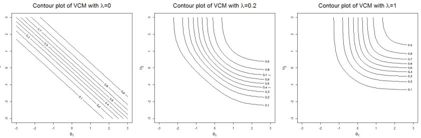
Swami-nathan, 2013). In MIRT, this probability is expressed by item response surface (IRS), which can be graphically displayed by probability contour plots in two-dimensional case (Ackerman, 1996). An example of contour plots of these three models are shown in Figure 2.1. The CM has linear and parallel equal probability contours. The NCM and VCM have curved equal probability contours.

Figure 2.1 The contour plots of compensatory (λ = 0), variable compensation (λ= 0.2) and non-compensatory (λ= 1) model,with a1 =a2 = 1 andb1 =b2 = 0.

2.2 Transformation Between Different Correlation Structures

For the compensatory model, an item can be graphically represented as an item vector ai (Reckase & McKinley, 1991). The length of the vector is the

multidimen-sional discrimination, MDISCi. In two dimensional case, it can be written as:

MDISCi = (a21i+a22i)1/2.

The direction of the item vector, measured by the angle of this vector from the positive θ1 axis, can be written as:

αi =arccos



 a1i

q a2

1i+a22i





1/2

(22)

Each angle represents a different composites of abilities in the (θ1, θ2) space. When

this angle is 0 or π/2, the item only measures one ability in the space. Otherwise, it measures both the two abilities in the space to some degree.

The compensatory model has no assumption on the correlation between θ1 and

θ2 (Ackerman, 1994). In this model, the space, or axes system, of the latent

abili-ties θ1 and θ2 can be arbitrarily rotated, simply using matrix multiplication. The

transformation from correlated to orthogonal abilities can be expressed by matrix multiplication (e.g., Oshima, Davey, & Lee, 2000; Smith, 2009):

θj = Σθ_j∗, (2.4)

whereθ∗ and θ are abilities values in correlated and uncorrelated spaces. The trans-formation (rotation) matrix is

Σ=



  

ψ1 ψ2

ψ2 ψ1



  ,

whereψ1 = √

1+ρ+√1−ρ

2 andψ2 =

√

1+ρ−√1−ρ

2 , with the correlation 06ρ61. To insure

the probability in (2.1) remains the same, a transformation of the discrimination parameters is needed:

at_i = (a∗_i)tΣ−1. (2.5) Since at

iθj = (a∗i)tΣ−1Σθ∗j = (a∗i)tθj∗, the probability of correct response given

by transformed and untransformed parameters are the same. Therefore, this trans-formation has no influence on model fitting.

Since Σ is an invertible matrix, this transformation is invertible. One can trans-form the parameter back to correlated space, simply exchanging the roles of Σ and

(23)

space, then to parameters under any other correlation structures. Therefore, trans-formations between any correlation structures are possible.

For graphical convenience, the θ1 axis is typically represented as orthogonal to

the θ2 (Ackerman, 1994). In plots, The effect of transformation is reflected in the

item vectors. With the transformation (Equation 2.4), the discrimination MDISCi

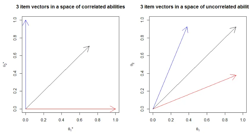
and the reference angle αi will change. Figure 2.2 demonstrates the transformation

between correlated space and uncorrelated space. In the correlated (θ₁∗, θ∗₂) space, the red and the blue item only measureθ₁∗andθ₂∗, respectively. The black item (with item vector in the middle) equally measures two abilities. As the abilities are transformed to uncorrelated space, the red (on θ1 axis) and the blue (on θ2 axis) item vector

are rotated towards the black item vector, thus measure both the two uncorrelated abilities (θ1, θ2). The direction of the black item remains the same, while its MDISCi

becomes greater in this space.

(24)

Since the transformation is one-to-one, parameters sets from two different correla-tion structures are also linked one-to-one. This transformacorrela-tion allows for estimacorrela-tion using an ability distribution with an arbitrary correlation. When interpreting the latent traits, one can transform the ability estimates using (Equation 2.4) to ensure that they have a certain correlation structure. This is not the case for the non-compensatory model and the variable compensation model. For those models, any transformation involving rotation changes the probabilities in the NCM (Equation 2.2) and VCM (Equation 2.3) due to their multiplicative structure. Therefore, wit-hout specifying the correlation structure between the latent traits, it is difficult to estimate and interpret the parameters in (Equation 2.2) and (Equation 2.3). As such, neither model has found wide use for analyzing real data sets. Similarly, the com-mon rotations in factor analysis and multivariate statistics, such as Varimax (Kaiser, 1958) and Procruste (Dean, 2000) rotation can be applied on the CM (e.g., Bolt & Lall, 2003), but not the NCM and VCM.

(25)

Chapter 3 Rotatable Asymmetric Variable Compensation

MIRT Model

3.1 The New Model and its Properties

To develop a non-compensatory MIRT model that allows for transformation bet-ween different correlation structures, we add additional discrimination parameters to the NCM (Equation 2.2). Because of the rotatability and flexibility of the new model, it is named the Rotatable Asymmetric Variable Compensation Model (RAVCM). It can be written as:

P(Xij = 1|a1i, a2i, a3i, a4i, b1i, b2i,θj)

= (

1

1 +exp[−1.7(a1iθ1j+a2iθ2j−b1i)]

)(

1

1 +exp[−1.7(a3iθ1j +a4iθ2j−b2i)]

) .

(3.1) The item response function of this new model can be viewed as a product of item response functions of two compensatory items. To avoid indeterminacy, it is assumed that the angle of the first item vector from the θ1 axis is smaller than the angle of

the second item vector. That is, a1i/(a21i +a22i) > a3i/(a23i +a24i). Similarly to the

compensatory model, the correlation structure in the RAVCM can be transformed via Equation 2.4, and the probability in (Equation 3.1) can be kept by transforming the two item vectors (a1i, a2i) and (a3i, a4i) by multiplying the inverse transformation

(26)

When a2i and a3i in the RAVCM (Equation 3.1) are 0, the new model (Equation

3.1) and the non-compensatory model (Equation 2.2) are the same. If the RAVCM (Equation 3.1) is non-compensatory with correlated abilities, its two item vectors are exactly on the θ1 and θ2 axes, respectively. After transforming the abilities to

uncorrelated space, the two items vectors are rotated towards the θ1 = θ2 line, and

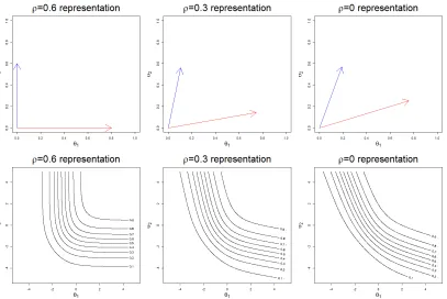
thus the RAVCM (Equation 3.1) is no longer a standard non-compensatory model in this uncorrelated space. Therefore, the NCM (Equation 2.2) is also a special case of the RAVCM (Equation 3.1), under a specific correlation structure. In the NCM, the true item parameters are unique, and they can be obtained only if this correlation is correctly specified. In the RAVCM, the item parameters can be recovered under any correlation structure. In Figure 3.1, the different representations of the same item in spaces with different correlation structures are shown. The item response function of the item is the NCM when ρ= 0.6.

The RAVCM cannot be exactly matched up with the compensatory model (Equa-tion 2.1) or the variable compensa(Equa-tion model (Equa(Equa-tion 2.3). However, like the VCM (Equation 2.3), the RAVCM (Equation 3.1) allows for different compensation levels. One extreme case is that when a1/a2 = a3/a4, it is compensatory with linear equal

probability contours. With proper parametrization, the item response surface of the CM (Equation 2.1) can be approximated well by the RAVCM (Equation 3.1). For any item in the CM with parametersa1,CM,a2,CM andbCM, let the parameters in the

RA-VCM bea1 =a3 = 0.739a1,CM,a2 =a4 = 0.739a2,CM andb1 =b2 = 0.739bCM−0.559,

(27)

fitted CM and RAVCM are very similar.

Figure 3.1 The different representation of item vectors and contour plots of a single item under spaces as viewed using different correlation structures.

Figure 3.2 The contour plots of: (a) CM with a1,CM = 1, a2,CM = 0.7 and

bCM = 0.5; (b) New model approximation witha1 =a3 = 0.739∗a1,CM,

a2 =a4 = 0.739∗a2,CM and b1 =b2 = 0.739∗bCM −0.559; (c) The overlapped

(28)

Figure 3.3 The contour plots of the probability difference of CM with a1,CM = 1,

a2,CM = 0.7 and bCM = 0.5 and RAVCM approximation with

a1 =a3 = 0.739∗a1,CM, a2 =a4 = 0.739∗a2,CM and b1 =b2 = 0.739∗bCM −0.559;

When 0 < a2 < a1 and 0 < a3 < a4, the contour plot of the RAVCM is similar

to the variable compensation model. Moreover, the RAVCM allows for asymmetric compensation, which means that the compensation levels can be different for diffe-rent portions of the ability distribution. When one of the item vectors is close to an axis, for example, the θ1 axis, and the other one is close to the line θ1 = θ2, the

compensation level of “θ1 to θ2” is larger than “θ2 to θ1”. In other words, when θ2 is

small, a large θ1 can raise the probability in (Equation 3.1), but when θ1 is small, a

largeθ2 cannot do the same thing effectively. One extreme example is that, ifa1 = 1,

a2 = 0,a3 = 1, a4 = 1, then θ1 can compensate for θ2 but θ2 cannot compensate for

θ1. In this case, one half of the contour plot is similar to the CM and the other half

is like the NCM (Figure 3.4). In this case, θ1 can compensate for θ2 but θ2 cannot

compensate for θ1. An example of asymmetric compensation could be a math test

(29)

enough math ability.

Figure 3.4 θ1 compensates θ2 only. The second plot is overlapped with CM (blue)

and NCM (red).

The RAVCM (Equation 3.1) can also be considered as a multi-step model since it is multiplicative. Its aparameters can be interpreted as the amount of ability used in each step. In terms of item response surface, (a1, a2) and (a3, a4) determines

the angle and density of the upper and lower half of the contours. As in Figure 3.4, when the first item vector (a1, a2) = (1,0) is on the θ1 axis, the top half of the

contours are perpendicular to the θ1 axis. The angle between the second item vector

(a3, a4) = (1,1) and the θ1 axis is 45 degree, so the angle between the lower half of

the contours and the θ1 axis is 45 degree. The second item vector is longer than the

first, therefore the lower half of the contours is denser.

(30)

model is the NCM (Equation 2.2). Since the compensation level is not stable under rotations that change the correlation structure, to compare those of different items, these angles should be obtained in the uncorrelated space.

3.2 Estimation of the RAVCM

3.2.1 Markov Chain Monte Carlo for Estimating MIRT Models

In recent research, Markov chain Monte Carlo (MCMC) methods have been wi-dely used to recover parameters of IRT models (e.g., Albert, 1992; Babcock, 2009, 2011; Baker, 1998; Beguin & Glas, 2011; Bolt & Lall, 2003; Kim & Bolt, 2007; Patz & Junker, 1999; Simpson, 2005). MCMC methods attempt to directly draw samples from the parameters’ joint Bayesian posterior distribution, and thus do not require any complicated calculations such as derivatives and integrals. Therefore, as model complexity increases, MCMC methods can still be easily applied, while the other methods such as marginal maximum likelihood (MML) with the EM algorithm (e.g., Bock & Aitkin, 1981) becomes too messy (Wollack, Bolt, Allan, & Lee, 2002).

(31)

enough unidimensional items on each dimensions. In their simulation, Babcock used 2, 6, or 10 unidimensional items and 50 multidimensional items; Chalmers and Flora had 5, 10, or 15 unidimensional items and 10 non-compensatory items. Wang and Nydick (2015) compared the performance of the MCMC and MH-RM on a different version of NCM (restricted C-MIRT) and concluded that the MCMC gives better esti-mates when the correlation between abilities are large. For the variable compensation model, Simpson (2005) estimated a simplified version of it (the G-MIRT model) with fixed discrimination parameters using MCMC through WinBUGS. The estimation results were not very satisfactory since many MCMC chains did not converge. The problem might be caused by the λ parameter. Note that, even with small λ (e.g., 0.2), the contour plot of the VCM can still be very similar to that of the NCM (e.g., Figure 2.1). Therefore, it is not easy to find an appropriate prior of λ. Fu (2015) suggested using ad-hoc prior distributions for λ to make its Markov chain converges.

The RAVCM (Equation 3.1) has a similar mathematical structure to the NCM (Equation 2.2). It does not contain the compensation parameter λ, and thus can avoid any problems due to it. The estimation challenge comes from its large number of parameters and great flexibility. Here, the estimation of the RAVCM is imple-mented via the Metropolis-Hastings algorithm within Gibbs sampling (e.g., Babcock, 2011; Patz & Junker, 1999). The parameters are first divided into several Gibbs sampling subsets, then generated iteratively by Metropolis-Hastings algorithm, with proper prior and proposal distributions.

(32)

implemented using the Rcpp, a package for writing and running C++ code in R. It can use the CPU more efficiently, and thus greatly increase computational speed. For 30 items and 1000 examinees, it only takes the Rcpp program about 20 minutes to run 30000 iterations on a normal personal computer with 3.20 GHz CPU, which is many times shorter than BUGS.

3.2.2 Settings and Details

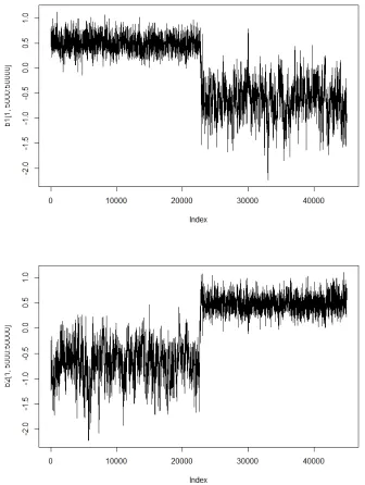
An estimation challenge of the RAVCM (Equation 3.1) is its indeterminacy. For the NCM (Equation 2.2), MCMC estimations may switch between the two dimensions over stages of the chains (Bolt & Lall, 2003). This means that at some point of the Markov chain, the parameters of one dimension come to represent those of the other dimension, and vice versa (e.g., Figure 3.5). An additional problem happens on the RAVCM is that the item parameters (a1i, a2i, b1i) and (a3i, a4i, b2i) can be exchanged

without changing the probability in (Equation 2.1), and without changing ability pa-rameters θ1j, θ2j. Thus, two types of “label switching” may happen on the RAVCM:

dimension label switching of all the parameters, and item parameter switching of pa-rameters of a single item. This may cause instability of the MCMC chains. To avoid the former type of “label switching”, identification constraints should be added. For the CM, this study uses a common method that is to fix the first item vector on the θ1 axis (e.g., Fraser & McDonald, 1988; Bolt & Lall, 2003). For the models containing

two item vectors, such as the RAVCM and its special case, the NCM, this study fixes only one vector on theθ1 axis, and let the other one be free, since in practice it is not

(33)

from theθ1 axis. (When this assumption is violated by the generated avalues in the

chain, these values are rejected with probability 1.) Additionally, the other settings and details of the MCMC estimation need to be adjusted carefully.

(34)

Gibbs Sampling Subsets

It is important to choose proper parameter subsets of Gibbs sampling to keep the balance between calculation speed and convergence speed. Although having fewer subsets lead to faster calculation in one iteration, more iterations are needed to stabi-lize the chain. Patz and Junker (1999) suggested putting all of the ability parameters in one subset and putting all of item parameters in the other subset. In this study, the ability parameters, discrimination parameters and difficulty parameters are divi-ded into three different subsets. One reason is that, compared to the NCM, it takes longer to get converging chains due to the additional discrimination parameters in the RAVCM. With more subsets, the acceptance rate of the Metropolis-Hastings can be adjusted by changing the variance of the proposal distribution separately for each group of parameters. This can make the chains converge faster.

Prior Distributions

As mentioned previously, it is assumed that the first item vector has smaller angle from the θ1 axis. The prior distributions of a3i and a2i should be set to be

stochas-tically smaller than, or equal to the priors of a1i and a4i, respectively. On the other

hand, to allow for more flexibility, the variance of the prior distributions ofa2i anda3i

should not be too small, unless it is known that the true model is close to the NCM. This study takes the truncated normal distribution with mean 1 and variance 1 as the prior distribution for a1i and a4i. (It is truncated such that thea parameters are

greater than 0.) Fora2i anda3i, it takes Exponential (1.5) when the true model is the

(35)

priors with covariance matrix equal to the identity matrix for the CM, and estimated the covariance matrix for the NCM. In this study, since the RAVCM (Equation 2.1) allows for transformation between correlation structures like CM, the covariance of the normal priors are set to be 0. Normal priors with mean 0 and variance 2 are assigned to the difficulty parameters.

Proposal distributions

(36)

3.2.3 Algorithm

Notations of this section

The whole test result is recorded by a matrix denoted by X. The result of item i answered by responser j is denoted by Xij, the element on row i and column j. It

is 1 when the answer is correct, 0 when the answer is incorrect. Then the row Xi is

a sequence of all examinees’ results for itemi and the column Xj is the results of all

items for examinee j.

The ability parameters of examinee j are denoted by the vector θj=(θ1j, θ2j).

The difficulty parameters are denoted by the vector bi=(bi1, bi2). Then

discrimina-tion parameters are denoted by the vector ai=(ai1, ai2, ai3, ai4). The vector of all

item parameters of item i is denoted by γi. Combining the parameters of all items

or examinees, we have the matrices θ, a, b, and γ. The variances of proposal distri-butions ofθ, a, and b parameters are denoted by c_θ2,c2_a and c2_b, respectively.

Algorithm

1. Generate θk

j fromp(θj|γk−1,X) for each j:

a. Generate θ∗_j = (θ∗₁_j, θ₂∗_j) from N(θk₁_j−1, c2

θ) and N(θ k−1

2j , c2θ) for each j.

b. For each j, accept θk j =θ

∗

j with probability

α(θ_jk−1,θ∗_j)

= p(Xj|θ

∗

j,γ k−1

j )π(θ∗)

p(Xj|θjk−1,γ k−1

j )π(θk−1) ∧1

= [ Q

iPij(θ∗j,γ k−1

i )Xij(1−Pij(θj∗,γ k−1

i ))1−Xij]exp(−

(θ∗₁_j)2₊₍_θ∗

2j)2

2 )

[Q

iPij(θkj−1,γk

−1

i )Xij(1−Pij(θjk−1,γk

−1

i ))1−Xij]exp(−

(θ₁k_j−1)2₊₍_θk−1 2j )2

2 )

∧1,

where Pij is given by Equation 2.1 in section 2.1. π is the prior distribution.

When θ_j∗ is rejected, takeθk j =θk

−1

(37)

2. Generate ak

i from p(a|θk,bk

−1_,_X_{) for each i:}

a. Generate discrimination parameters (a∗_il) from N(ak_il−1, c2

a) separately for each i,

where l= 1,2,3,4. b. For each i, accept ak

i =a

∗

i with probability

α(ak_i−1,a∗_i)

= [ Q

jPij(θk,a∗i,b k−1

i )Xij(1−Pij(θk,a∗i,b k−1

i ))1−Xij]

Q4

l=1π(a ∗

il)

[Q

jPij(θk,aki−1,bk

−1

i )Xij(1−Pij(θk,aki−1,bk

−1

i ))1−Xij]

Q4

l=1π(a

k−1

il ) ∧1.

When a∗_i is rejected, take ak_i =ak_i−1

3. Generate bk

i from p(b|θk,ak,X) for each i:

a. Generate difficulty parameters (b∗_il) from N(bk_il−1, c2

b) separately for each i, where

l = 1,2.

b. For each i, accept bk_i =b∗_i with probability

α(bk_i−1,b∗_i)

= [ Q

jPij(θk,aki,b∗i)Xij(1−Pij(θk,aik,b∗i))1−Xij]

Q2

l=1π(b ∗

il)

[Q

jPij(θk,aki,bk

−1

i )Xij(1−Pij(θk,aki,bk

−1

i ))1−Xij]

Q2

l=1π(bk −1

il ) ∧1.

When b∗_i is rejected, take bk i =b

k−1

i .

4. Repeat step 1, 2 and 3 with a large number of iterations (e.g., 30000).

3.3 Simulation

(38)

are estimated by the same method, i.e., Metropolis Hasting within Gibbs sampler. The choices of prior distributions are also similar. When estimating the CM, NCM, and VCM, the prior distributions of a, b, and θ are set to be normal, which is the same as the priors of the RAVCM. In different simulations, the ability parameters (θ1, θ2) are all generated from multivariate normal, with different correlation. The a

parameters are generated from the truncated normal distribution with mean 1 and variance 1. To keep the monotonicity of the model, it is assumed that a parameters are not smaller than 0. If a generated value is negative, it will be re-generated. The difficulty parameters (b) are generated from normal distribution with variance 1.5 and mean 0 for the CM, mean -1 for the NCM, due to the large overall difficulty of the NCM (Bolt & Lall, 2003).

(39)

The following statistics are included in the results. The first one is root mean square errors (RMSEs) of ability estimates, defined as

RMSE(θ.) =

v u u u t 1 N N X j=1

(θ.j −θˆ.j)2,

whereN is the total number of examinees;θ.jand ˆθ.jare the true ability and estimates

ability of the j-th examinees, respectively. The point “.” can be replaced by any dimension number, such as 1 or 2 in two-dimensional case. Second, RMSEs of the estimated response surfaces, which is

RMSE( ˆP(θ)) = v u u u t 1 nN n X i=1 N X j=1

(Pij(θj)−Pˆij(θj))2,

where n and N are the number of items and examinees, respectively. Pij(θj) and

ˆ

Pij(θj) are probabilities that examinee j answers item i correctly, given by the true

and estimated item response surface of item i, respectively. The two probabilities are both evaluated using true abilities, and thus only measure how well the item re-sponse surfaces are recovered. Unlike the integral over the whole space, this statistic measures the differences between the true and estimated surfaces where the abilities exist. The last statistic is log-likelihood of the estimated model, which is a measure of goodness of fit. The statistics in the results are based on an average of 50 replications, for each setting.

(40)

sur-faces as well as the CM (It might be caused by the difference between the CM and RAVCM surfaces.), it gives much smaller RMSEs than the NCM. Also, the ability RMSEs of the RAVCM is very similar to those of the CM. When the NCM is the true model, the log-likelihoods given by the three models are close, but the RMSEs of ability estimates and surfaces given by the CM are generally larger than the NCM and RAVCM. When half of items are generated from the CM and the other half are generated using the NCM, the RAVCM gives smaller RMSEs of ability and surface estimates than the CM and the NCM.

Table 3.1 Performance of the CM, NCM and RAVCM when the true model is the CM. (“R” is the abbreviation of “RMSE”. “Fitted” means the fitted model.)

Sample Size Fitted R(θ1) R(θ2) SE(θ1) SE(θ2) R( ˆP(θ)) Log like

500 examinees CM 0.58 0.59 0.59 0.81 0.04 -2218 15 items NCM 0.67 0.67 0.69 0.79 0.24 -3637 RAVCM 0.59 0.59 0.69 0.72 0.08 -2335 500 examinees CM 0.48 0.55 0.46 0.75 0.03 -4739 30 items NCM 0.57 0.65 0.67 0.73 0.16 -5026 RAVCM 0.50 0.57 0.59 0.68 0.08 -4915 1000 examinees CM 0.63 0.65 0.55 0.91 0.03 -4749 15 items NCM 0.73 0.73 0.80 0.83 0.16 -5313 RAVCM 0.65 0.66 0.48 0.99 0.07 -4997 1000 examinees CM 0.52 0.53 0.40 0.72 0.03 -10107

30 items NCM 0.61 0.62 0.63 0.64 0.14 -10478 RAVCM 0.52 0.53 0.55 0.60 0.07 -10663

(41)

Table 3.2 Performance of the CM, NCM and RAVCM when the true model is the NCM. (“R” is the abbreviation of “RMSE”. “Fitted” means the fitted model.)

30 items NCM 0.55 0.58 0.58 0.63 0.04 -11045 RAVCM 0.56 0.59 0.60 0.61 0.07 -11132

the abilities are correlated. Under all conditions, the RAVCM gives smaller RMSEs of abilities than the NCM. The RMSEs of surfaces are similar. It indicates that after transforming the estimates to correlated space, the RAVCM gives surfaces close to the NCM, which means that the true surfaces in uncorrelated space are well recove-red. The log-likelihood of fitted RAVCM is smaller than the NCM when the number of items are small (15). With 30 items, the log-likelihoods are similar.

(42)

Table 3.3 Performance of the CM, NCM and RAVCM when the true model is the mixture of the CM and NCM. (Half of items are generated using the CM, and the other half are generated using the NCM). (“R” is the abbreviation of “RMSE”. “Fitted” means the fitted model.)

True Model: 7 CM items, 8 NCM items or 15 CM items, 15 NCM items. Sample Size Fitted R(θ1) R(θ2) SE(θ1) SE(θ2) R( ˆP(θ)) Log like

30 items NCM 0.51 0.55 0.54 0.62 0.08 -11075 RAVCM 0.47 0.49 0.50 0.58 0.05 -11077

Table 3.4 Performance comparison between the NCM and RAVCM when abilities are correlated. Parameter recovery of the RAVCM was evaluated after transforming the estimates back onto the simulated scales where the abilities are correlated. The true correlation is 0.4.

500 examinees NCM 0.73 0.75 0.94 0.95 0.12 -3282 15 items RAVCM 0.67 0.68 0.87 0.94 0.12 -2789 500 examinees NCM 0.52 0.55 0.59 0.62 0.05 -5933 30 items RAVCM 0.48 0.50 0.59 0.58 0.06 -5908 1000 examinees NCM 0.65 0.69 0.90 0.88 0.12 -7403 15 items RAVCM 0.62 0.63 0.82 0.87 0.12 -6648 1000 examinees NCM 0.52 0.53 0.60 0.66 0.05 -11811

30 items RAVCM 0.46 0.49 0.61 0.64 0.06 -11874

(43)

Table 3.5 Performance comparison between the NCM and RAVCM when abilities are correlated. Parameter recovery of the RAVCM was evaluated after transforming the estimates back onto the simulated scales where the abilities are correlated. The true correlation is 0.7.

500 examinees NCM 0.65 0.68 0.94 0.95 0.18 -4182 15 items RAVCM 0.51 0.55 0.69 0.79 0.18 -3699 500 examinees NCM 0.60 0.61 0.80 0.87 0.11 -6582 30 items RAVCM 0.49 0.52 0.79 0.83 0.11 -6372 1000 examinees NCM 0.56 0.60 0.82 0.85 0.08 -6418 15 items RAVCM 0.50 0.54 0.77 0.85 0.09 -5758 1000 examinees NCM 0.55 0.57 0.71 0.72 0.06 -12781

30 items RAVCM 0.45 0.47 0.66 0.73 0.07 -12754

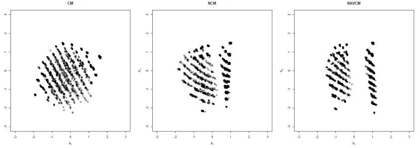
Figure 3.6 Contour plots of the true and estimated RAVCM under different spaces.

(44)

mis-specified correlation 0 and the transformed estimated RAVCM under the space where the correlation is 0.7 (the second column); (c) estimated standard NCM when corre-lation was specified as 0 and 0.7 (the third column). The label of the horizontal and vertical axis are θ1 andθ2, respectively. The true correlation of the generated ability

parameters was 0.7. All plots are for the same item.

3.4 A Real Data Study: Diagnostic Geometry Assessment

3.4.1 Overall Fitting and Interpretation

The CM, NCM and RAVCM were fit to a real data set from the Diagnostic Geometry Assessment project. This test is used by Measured Progress to identify three common misconceptions that their students hold in geometry (Shape Proper-ties, Transformations, and Geometric Measurement). The geometric measurement part of the test (1995 examinees, 10 items) is analyzed in the current study since it is used to measure two abilities: 1) the process of mentally structuring space; and 2) the connection between mental structuring and measurement formulas. Each item is about measuring the area of a figure using “unit figures” and/or formulas. Most items are multiple choice questions, while item 847 has three true-false sub-items. All items are related to structuring space, while items 851, 855 and 859 do not require knowledge of formula. A hierarchical cluster analysis (Roussos, Stout, & Marden, 1998) of the test also suggests that the test is related to two latent traits (Figure 3.7).

(45)

Figure 3.7 Dendrogram obtained from hierarchically clustering the DGAM data with complete linkage and Euclidean distance. Items 851, 855, and 859 are the only ones that lack formulas, but all of the items are related to structuring space.

number of tiles. To answer the question correctly, one only needs to know one of the two methods. Thus, the item seems compensatory. One the other hand, item 847 can be considered as non-compensatory, since one needs both abilities to answer all three sub-items correctly.

The CM, NCM and RAVCM are fit to the data. For the CM, according to some preliminary fitting results and the cluster analysis, item 851 fixed on theθ1 axis since

(46)

Table 3.6 reports item estimates given by the three models. From the CM so-lution, the items 851, 855 and 859 tend to measure the first ability only, which can be interpreted as the ability of mentally structuring space. The other items tends to measure both abilities, i.e., structuring space and connection between structuring and formulas. For the RAVCM, the pattern of estimatedb parameters are generally similar to the NCM estimates, while some estimated a parameters are not. Some items, such as item 851, 855, and 871 appears to be non-compensatory. The others appear similar to compensatory, or even asymmetrically compensatory items. For example, item 847 has similar â1 and â2, small â3 and large â4. It means that θ2

can compensate for θ1 but θ1 has difficulty compensating for θ2. For item 859, a

discrimination parameter estimated by the RAVCM is very large ( ˆa1 = 3.67). The

NCM also gives a large estimate ( ˆa1 = 4.97), while the CM gives small estimates

( ˆa1 = 0.67, ˆa2 = 0.03). The item response surfaces given by the three models are

very different (Figure 3.8). The CM is almost not related to θ2. The NCM requires

examinees to have enough θ1 and also θ2 to answer the question correctly. The

esti-mated surface given by the RAVCM is asymmetrically compensatory. How large θ1

is required depends on the value of θ2. To have high probability of correct response,

large θ1 is required when θ2 is very small. For example, when θ2 is -3, θ1 needs to

be about 2 to have 90% probability of correct response. When θ2 is large, less θ1 is

required.

(47)

Figure 3.8 The contour plots of the item response surfaces estimated by the CM, NCM and RAVCM for item 859.

Figure 3.9 Estimated ability distribution of the CM, NCM and RAVCM.

3.4.2 Item Fit and Person Fit

(48)

Table 3.7 Item log-likelihoods given by CM, NCM, and RAVCM fitted to the DGAM data.

851 855 859 839 843 847 863 867 871 879 CM -910 -1007 -1078 -985 -960 -901 -1013 -917 -1033 -877 NCM -1055 -1033 -641 -960 -934 -886 -1019 -946 -1030 -906 RAVCM -1059 -999 -414 -960 -956 -882 -1021 -956 -1038 -941

Total CM -9681 NCM -9410 RAVCM -9226

Drasgow, Levine and Williams (1985) proposed a standardized person fit statistic for unidimensional 3PL model, which is z3 = l

−E(l)

(V ar(l))1/2. l is the log-likelihood for

a person’s response. It and its moments are calculated using estimated parameters. Asymptotically, z3 is standard normal, and its square has chi-squared distribution

with degree of freedom 1. To use z3 as an item fit statistic, one can replace person

log-likelihood by item log-likelihood. Table 3.8 shows the squaredz3 statistics at the

item-level. Generally the RAVCM has the smallestz2

3. Figure 3.11 gives the

quantile-quantile plot of z2

3 given by the three models. High z32 indices indicate poor fit. For

the DGAM data, the CM and RAVCM gives better person fit than the NCM. Note that all points are below the q-q line. It might be caused by the small number of items (Molenaar & Hoijtink, 1990). In this case person fit statistics tend to be conservative.

Table 3.8 Drasgow’s z2

3 for each item given by CM, NCM, and RAVCM fitted to

the DGAM data.

(49)

Table 3.6 The CM, NCM and RAVCM item parameter estimates for the DGAM data. Parameters are scaled such that the variance of ˆθ1 and ˆθ2 is 1.

Item CM NCM RAVCM

ˆ

a1 aˆ2 ˆb aˆ1 aˆ2 bˆ1 bˆ2 aˆ1 aˆ2 aˆ3 aˆ4 bˆ1 bˆ2

851 0.99 0.00 0.00 0.89 0.75 -0.50 -0.50 0.87 0.00 0.16 0.63 -0.50 -0.50 855 0.76 0.14 0.11 0.94 0.73 -0.88 -0.46 1.11 0.04 0.03 0.77 -1.18 -0.35 859 0.67 0.03 -0.01 4.97 0.63 -0.59 -1.40 3.67 0.60 1.13 0.56 -0.43 -0.93 839 0.65 0.34 -0.41 1.39 0.81 -2.78 -0.41 0.52 0.44 0.04 0.80 -1.48 -0.71 843 0.71 0.27 -0.56 1.54 0.70 -2.39 -0.75 0.69 0.46 0.10 0.67 -1.27 -1.06 847 0.64 0.38 -0.77 0.78 0.92 -2.27 -0.78 0.35 0.54 0.07 0.75 -1.45 -1.22 863 0.55 0.38 -0.38 1.05 0.71 -2.13 -0.29 0.60 0.31 0.07 0.72 -1.62 -0.54 867 0.53 0.57 -0.55 0.88 0.84 -2.31 -0.42 0.44 0.45 0.05 0.77 -1.62 -0.69 871 0.54 0.65 -0.05 0.68 0.82 -1.48 -0.08 0.60 0.08 0.02 0.83 -1.54 -0.20 879 0.48 0.55 -0.77 0.13 0.90 -1.32 -1.19 0.24 0.58 0.08 0.56 -1.19 -1.31

(50)

Sinharay (2006) suggested using a Bayesian item fit diagnostic plot to check mo-del fitting, based on the posterior predictive momo-del-checking (PPMC) method (Rubin, 1984). The method generates replicated responses using parameters drawed at each iterate of the MCMC chain. In an item fit plot, the solid line connects points that indicates observed proportion correct of each raw score group. A box represents the distribution of replicated proportions correct. For any item, too many observed pro-portions lying far from the center of the replicated values indicate a failure of the model to explain the responses to the item. Figure 3.10 shows inadequate fit of the CM for item 859 since some boxes are far away from the line. For the NCM and RA-VCM, the observed proportions lie closer to the center of the boxes, which indicates better fit. For the other items, the fit plots of the three models are similar.

Figure 3.10 Item fit plot for item 859. The observed and replicated proportions correct are plotted for each raw-score group. The left panel (for the CM) shows sign of misfit while the middle and right panels (for the NCM and RAVCM,

(51)

Figure 3.11 Q-Q plot of z2

3 person fit statistics given by the CM, NCM and

RAVCM. The lower and higher horizontal dashed line of reference marks the 5% and 1% cut-off ofχ2 _{distribution, respectively.}

(52)

3.4.3 An Exploratory Simulation Study

It is doubtful that the item log-likelihood can really distinguish between the com-pensatory and non-comcom-pensatory items, especially when the number of items is small (see the next chapter). A method to explore the true model for each item is simu-lation. We can simulate data using different true models, and compare the pattern of log-likelihoods given by the estimated models with the log-likelihoods in the last section. When the models used to generate items are or similar to the true models, the likelihood pattern given by the fitted model with simulated data should be similar to the pattern in Table 3.7. The purpose of this exploratory simulation study is to find such models that can generate data similar to the real one. In this case we can claim that these models are close to the true models of the items.

(53)

Table 3.9 Item log-likelihoods given by CM, NCM, and RAVCM fitted to the DGAM data. Item responses are generated using the RAVCM for item 859. The others are generated using the CM.

851 855 859 839 843 847 863 867 871 879 CM -612 -876 -361 -808 -816 -830 -1033 -922 -1019 -832 NCM -1015 -830 -242 -828 -855 -844 -1021 -956 -1048 -853 RAVCM -596 -901 -405 -825 -842 -852 -1039 -931 -1018 -841

Total CM -8109 NCM -8492 RAVCM -8250

The following simulation shows that to obtain log-likelihood similar to those in the real data it is necessary to simulate more items using the NCM or RAVCM. Table 3.10 shows the log-likelihoods with a pattern more similar to the log-likelihoods for the real data. In this generated data set, only responses for 4 items are generated using the CM. 4 and 2 items are generated using the NCM and the RAVCM, respecti-vely. To some extent, this study shows that some items are indeed not compensatory, and are better fit by a model that accounts for that.

Table 3.10 Item log-likelihood given by CM, NCM, and RAVCM fitted to another simulated data. The responses of item 839 and 859 are simulated using the

RAVCM. The responses of item 871, 855, 863, 867 are simulated using the NCM. The responses of the other items are simulated using the CM.

851 855 859 839 843 847 863 867 871 879 CM -731 -1022 -612 -811 -820 -847 -839 -1004 -834 -855 NCM -1045 -994 -362 -825 -858 -860 -782 -789 -809 -882 RAVCM -1089 -997 -252 -816 -826 -894 -868 -732 -838 -866

(54)

3.5 Discussion: Definition of Compensation and Model

Interpretation

In literatures, the MIRT models are classified as compensatory and noncompen-satory (e.g., Ackerman, 1989; Bolt & Lall, 2003; Way, Ansley, & Forsyth, 1988). Traditionally, compensation is defined as “High ability on one dimension can com-pensate for the low ability on the second dimension” (e.g., Ackerman, Gierl, & Walker, 2003). The compensation level is described by a parameter λ in the variable com-pensation model GMIRT (Ackerman & Bolt, 1995; Simpson, 2005). This work put the compensatory model and the non-compensatory model into the same framework, and proposes a new possible type of compensation: in the middle of compensatory and non-compensatory.

An issue with the traditional definition and measure of compensation is the defini-tion of “high ability” and “low ability”. These two terms show that the compensadefini-tion depends on the value of “compensated ability” and “compensator ability”. For exam-ple, for a non-compensatory item (Figure 3.12), ifθ1 is very small (e.g., -3), then the

probability of correct response will not increase asθ2increase, for almost anyθ2 value.

However, ifθ1 is “a little small” (e.g., 0), the probability can increase from 0 to about

0.5 as θ2 increases from a small value. In the second case, θ2 does compensate for θ1

whenθ2 is small (e.g., -3), whileθ2cannot compensate forθ1 anymore when it is large

(55)

Figure 3.12 A non-compensatory example to explain the definition of compensation.

If the compensation depends on the values of abilities, then it might be difficult to give all information about compensation using a single parameter, for example, the compensation parameterλ in the VCM. For example, even if two items are both compensatory (with λ = 0), their compensations can be different, as stated in (Ac-kerman, Gierl, & Walker, 2003): “compensation is greatest when an item has equal discrimination parameters.” Figure 3.13 shows an example. The two items are both compensatory with linear contours. The first item has discrimination parameters a1 =a2 = 1; the second item has a1 = 1, a2 = 0.2. For the first item, θ1 and θ2 can

compensate for each other, while for the second item, ifθ1 is low, the the probability

of correct response will not increase a lot as θ2 increases. From this examples, it can

(56)

Figure 3.13 Two compensatory items to explain the definition of compensation.

Since compensation depends on the compensator and the values of abilities, it can be redefined by a question: “With fixed abilities on compensated dimensions, how fast does the probability of correct response increase as the compensator incre-ases?” “How fast” can be mathematically described using derivatives, for example,

∂P(θ1,θ2,θ3,...)

∂θ1 can be considered as the function of compensation level with

compensa-tor θ1. If the other abilities are fixed, it will be a function of θ1. This definition is

formal, however, and hard to interpret. One can never list the derivatives of the item response function for all possible compensators and values of abilities.

(57)

compensation structure such as the CM or the NCM, the decision is based on their assumptions on how the abilities combine, or cognitive strategies (Ackerman & Bolt, 1995).

In reality, the shape of the contour plot almost surely differs at least somewhat from the linear contour plot for the CM and the curved contour plot for the NCM. For example, the contour could be asymmetric as shown in Figure 3.4. If a model is too restrictive, then it cannot fit every item well, which leads to inaccurate or invalid ability estimates. It is important to have a MIRT model flexible enough to approxi-mate more types of contour plot. This makes the RAVCM potentially useful in that it can approximate more types of contour plot than the common existing MIRT models. As seen in some cases, it gives better ability estimates than the existing MIRT models.

The RAVCM also solves the problem that the compensation of an item can change via rotation. For the same item, the contour plots under different correlation structu-res can be highly different, as shown in Figure 3.6. If the model is rotatable, then the compensation of items can be compared even if they are under different space. For example, if item 1 and item 2 are non-compensatory when the correlations of abilities are 0.6 and 0.3 respectively. Under the framework of the NCM, their compensations are not comparable, while under the framework of the RAVCM, one can transform the items to the uncorrelated space to compare their compensation.

(58)

(59)

Chapter 4 Evaluating Competing MIRT Models with

Different Goodness of Fit Statistics

Model and item misfit often lead to biased estimates and inappropriate interpreta-tions for parameters in item response theory. Traditionally, the reason of item misfit are considered coming from the violation of one of the three assumptions of IRT, or model misspecification (Levine & Rubin, 1979). Model mis-specification can include violation of item response functions (Orlando & Thissen, 2003) and aberrant response patterns (Drasgow, Levine, & McLaughlin, 1991). In the past decades, many good-ness of fit test and statistics are developed to evaluate the IRT model fitting, such asQ1 (Yen, 1981),Z3 (Drasgow, Levine, & Williams, 1985), and S−χ2 (Orlando &

Thissen, 2000). These statistics are designed for unidimensional IRT models. There are relatively less research for the goodness of fit test and statistics for MIRT models. One example is Zhang & Stone (2008), which examine the utility of the S−χ2

like-lihood based statistic in evaluating item fit for the compensatory model. The item misfit in their research are caused by the violation of the monotonicity assumption and ignored guessing effect, which have been studied for unidimensional IRT models. However, in addition to these common threats to goodness of fit in unidimensional IRT, mis-specifying the compensation in MIRT can cause model or item misfit. As this type of item misfit is not studied in Zhang & Stone (2008), their conclusion that the S−χ2 _{statistic is capable of evaluating item fit in the CM might not be always}

(60)

In practice, the compensatory model is widely applied. However, as showed in table 3.2, when the compensatory model is fit, but the true model is the non-compensatory model, the RMSEs of estimated parameters can be large. Also, using the compensatory model for non-compensatory items is considered as a cause of dif-ferential item functioning (DIF; Liaw, 2015). In this case, the CM does not measure the true latent traits that generate the data, which is what the test maker want to measure. In real data analysis, RMSEs is unavailable. It would be good if there was a powerful goodness of fit test that could reject the CM with large probability. So, when different MIRT models are fit, statistics for model selection are needed.

The purpose of this study is to evaluate the effectiveness of goodness of fit statistics at distinguishing between the compensatory model and the non-compensatory model at the test-level and the item-level via simulation. Since the RAVCM can approxi-mate both the CM and the NCM, it is also important to check if it can outperform the statistics in distinguishing the compensatory and non-compensatory items.

4.1 Statistics in this Study

The statistics evaluated in this study are the M2 (Maydeu-Olivares & Joe, 2005),

S − χ2 (Orlando & Thissen, 2000), Z3 (Drasgow, Levine, & Williams, 1985), log