ABSTRACT
SHAH, KUNAL DEEPAK. Image Processing for Cognitive Models in Dynamic Gaming
Environments. (Under the direction of Dr. Robert St. Amant).
Cognitive models have typically dealt with environments that are either artificial or real
but too simplistic. This stems from the fact that the process of describing the environment
to the cognitive model is a complex vision problem. In order to realize the full potential
of cognitive models, it is imperative that they be able to operate in natural domains. We
attempt to overcome this limitation by providing a perceptual component to a cognitive
model that interacts with more realistic environments. This perceptual component is an
image processing substrate that has been customized for two different gaming
environments. The substrate formerly worked only for the static environments we
associate with conventional graphical user interfaces; the work we describe here extends
its functionality to a more general class of interfaces, as represented by the driving game
and Mars rover game. A cognitive model built on the ACT-R cognitive architecture has
been developed that demonstrates the use of the image processing substrate in performing
IMAGE PROCESSING FOR COGNITIVE MODELS IN DYNAMIC GAMING ENVIRONMENTS
by
KUNAL DEEPAK SHAH
A thesis submitted to the Graduate Faculty of North Carolina State University
in the partial fulfillment of the requirements for the degree of
Masters of Science
COMPUTER SCIENCE
Raleigh, NC
June 19, 2003
APPROVED BY:
________________________ _______________________
Dr. Michael Young Dr. Munindar Singh
_____________________
Dr. Robert St. Amant
Biography
Kunal Shah was born on August 7, 1980 in Mumbai, India. He graduated with a Bachelor
of Engineering degree in Information Technology from Nirma Institute of Technology
(Gujarat University), Ahmedabad in June 2001. He worked as a Project Intern with Tata
Consultancy Services, Mumbai as part of his final semester project. He then joined the
Masters program in Computer Science at North Carolina State University. While working
towards the Masters degree, he also spent summer and fall 2002 interning with Allied
Acknowledgements
I thank my advisor, Dr. Robert St. Amant for his constant guidance and advice, without
which this thesis would not have been possible. I express my gratitude to Sameer
Rajyaguru, who had been working with me on the same project and shared a lot of ideas
with me. I would also like to thank Arnav Jhala, whose insights into this project helped
me come up with a solution better than what it would have been otherwise. Finally, I
wish to thank my committee members, Dr. Munindar Singh and Dr. Michael Young for
Contents
LIST OF FIGURES... VI
LIST OF TABLES... VII
1. INTRODUCTION ... 1
1.1MOTIVATION... 1
2. VISUAL ENVRIRONMENTS FOR COGNITIVE MODELING ... 7
2.1CLASSIFICATION OF GAMES... 7
2.2GAMES WE CONSIDERED... 14
3. RELATED WORK... 16
3.1VISUAL RECOGNITION IN HUMANS... 17
3.1.1 Low Level Vision... 18
3.1.2 Intermediate Level Vision ... 20
3.1.3 High Level Vision... 20
3.2IMAGE PROCESSING FOR OBJECT RECOGNITION... 21
3.2.1 Preprocessing ... 22
3.2.2 Data Reduction & Morphological Filtering ... 23
3.2.3 Feature Extraction and Analysis... 31
4. THE SYSTEM ... 40
4.1SYSTEM DESIGN... 40
4.1.2 Generic Core... 42
4.2MARS ROVER... 48
4.2.1 Cognitive Model Requirements... 49
4.33D-DRIVER... 55
4.3.1 Cognitive Model Requirements... 56
4.3.2 Approach... 57
4.4RESULTS AND EVALUATION... 64
5. CONCLUSIONS AND FUTURE WORK... 66
List of Figures
FIGURE 1:3D-DRIVER... 14
FIGURE 2:MARS ROVER... 14
FIGURE 3.ORIGINAL IMAGE FOR SEGMENTATION... 28
FIGURE 4.HISTOGRAM... 28
FIGURE 5.THRESHOLDING (Θ=94)... 28
FIGURE 6.ORIGINAL IMAGE FOR SHAPE DETECTION... 38
FIGURE 7.EDGE DETECTED IMAGE... 38
FIGURE 8.HOUGH SPACE... 38
FIGURE 9.CENTER OF CIRCLE OBTAINED USING HOUGH TRANSFORM... 38
FIGURE 10.ARCHITECTURAL DIAGRAM OF THE SYSTEM... 41
FIGURE 11.CONTROL FLOW DIAGRAM OF GENERIC CORE... 43
FIGURE 12.DRIVING ENVIRONMENT WITHOUT ANY IMAGE PROCESSING... 45
FIGURE 13.DRIVING ENVIRONMENT AFTER NORMALIZATION AND QUANTIZATION... 45
FIGURE 14.DRIVING ENVIRONMENT WITHOUT ANY IMAGE PROCESSING... 46
FIGURE 15.DRIVING ENVIRONMENT AFTER EDGE DETECTION... 46
FIGURE 16.SCREEN CAPTURE OF MARS ROVER... 49
FIGURE 17.SCREEN CAPTURE OF 3D-DRIVER... 55
List of Tables
1. Introduction
This thesis addresses the issue of developing image-processing algorithms that meet the
needs of cognitive models, while adhering to the theory of human vision to a certain
extent. The focus is on an image processing system that has been coupled with the
ACT-R[1] cognitive modeling architecture. The system supports interaction with
dynamically changing visual environments associated with an off-the-shelf computer
game that runs independently of the model. The image processing techniques have been
tailored to two different games and are intended to be extensible to others. This thesis
discusses the image processing approach, its strengths and limitations, and its
implications for cognitive modeling in more naturalistic environments. It also sheds
light on the design issues to be considered for different gaming domains, the tradeoffs
to be made in modeling human vision by computational means for efficiency in playing
games and the changes necessitated by dynamic environments in a system such as
SegMan[2] for its use in such environments.
1.1 Motivation
Cognitive models are systems that attempt to explain human cognition through the
explicit representation of knowledge structures and processing. A cognitive model is a
computational model of human information processing. Cognitive models commonly
include components analogous to processes studied by psychologists, including working
memory and long-term memory processing, perception and motor action. The earliest
such as being able to retrieve specific information from memory. Gradually, however,
cognitive modelers have come to rely on unified modeling architectures that attempt to
capture most or all of the phenomena that fall under the category of cognitive processing.
Models created in these architectures simulate human behavior by committing errors and
taking time to perform actions. For example, each covert step of cognition and overt
action has latencies associated with them that are based on psychological theories and
data. Some of the well-known cognitive architectures that have been used in practice are
Soar, ACT-R and EPIC. It is possible to build any number of cognitive models within a
given architecture, which can then be combined to model any complex processing
activity.
These cognitive models have a number of uses. They help cognitive modelers validate
predictions made by psychologists about human behavior and thereby better understand
the human behavior, in the same way that ergonomics researches work with models of
human physiology or civil engineers work with models of bridges before they build them.
Cognitive models also provide a means of applying knowledge about human behavior to
the design of user interfaces, thereby helping in improving their quality and usability
[Citation]. Particularly, cognitive models have been used in three main ways. They have
been used as surrogate users that show how different designs lead to different behaviors
and why users have trouble with particular activities. Such cognitive models have been
used to populate synthetic environments, for example fighter aircraft crews[32] and also
as simulated users to test interfaces[33]. They have also been used as embedded assistants
such models that have been used in school education[31]. They encapsulate the
knowledge about the task that the student is attempting and provide specialized support
based on that knowledge. Finally, they have been used for predicting some aspects of
human performance such as time and errors with a given interface, thereby helping in
creation of better designs. Keystroke Level Model and GOMS family of models are such
models that have been deployed successfully[29].
A basic concern in cognitive modeling is the representation of problem-solving
environments. Ideally, we want an environment that the model lives in to reflect all of
the relevant details that humans are aware of and constrained by in carrying out a task.
The most direct way of satisfying this goal is to build models that can interact with the
real world. In most of the early cognitive models, the interaction was based on hooks
provided by the interface, bypassing the complex visual processing that occurs in
humans. For some cognitive modeling systems, visual input was generated via the
look-up of properties in a hand-constructed interface specification. Other models interacted
with dynamic simulations of interfaces, constructed to mimic the behavior of a real
interface, but tailored to the input and output requirements of the model. The drawback of
these approaches is that there are built-in biases when a model interacts with a simulation
or hand-built environment. Interface simulations and specifications are abstractions; they
do away with details of a real interface that may or may not be important. Real user
interfaces exhibit variation in timing, predictability and reliability of actions, and the
performance on a given task. Neglecting these subtleties can bring the validity of
empirical cognitive modeling results into question.
A more general approach is to allow direct access to input and output devices, such as
display screen and the mouse. Doing so provides a way for a model to manipulate all
interfaces in an interactive system. Such a mechanism would be ecologically valid and
save a lot of effort that goes into the development of simulated or hand-built interfaces.
However, the cognitive model now needs to address a new set of complexities dealing
with visual processing, object manipulation and so forth. Recent research efforts have
adopted the modest goal of building cognitive models that can interact with software
environments designed for human users. Everyday productivity applications contain text,
numbers, and discrete objects and symbols in relatively simple arrangements; these
environmental properties make it feasible, sometimes even straightforward, to
accommodate the input requirements of a symbolic cognitive model. SegMan[2] is such a
system designed to interact with Microsoft Windows graphical direct-manipulation
interface. It is a perceptual substrate that uses computational vision to "see" the
environment. SegMan enables other programs to be able to see the graphical interface
screen as a human would see it. It takes pixel-level input from the display, runs the data
through image processing algorithms, and builds a structured representation of visible
interface objects. This enables programs to interact with Microsoft Windows as if it were
a user sitting at the console instead of relying on low-level APIs. However, SegMan is
limited in its applicability to a wider range of interfaces because it relies on the
For example, Microsoft Windows graphical user interface is highly rectilinear and highly
standardized. Even, the components such as buttons and other controls are rectangular,
with lined borders and shadows.
Such environments are relatively simple in comparison with natural environments. They
tend to be static, discrete, and predictable, properties that can be exploited by a model but
that simultaneously limit the range of results that can be reached in experimenting with
them. Hence, the image processing algorithms for such environments do not require
sophisticated techniques. In order to realize the full potential of cognitive models, it is
imperative that they be operable in natural environments. Our work attempts to overcome
this limitation, by building models that can interact with computer based video games.
Our system extends the functionality of SegMan to a more general class of interfaces, not
merely static environments. Games are representative of such environments and we
believe that if we are able to apply cognitive models in such dynamic games, then they
can easily be applied to general interfaces as well. Games have played an important role
in helping cognitive modelers gain insight into the process of human reasoning.
Historically, strategy games such as tic-tac-toe and chess have led to an improved
understanding of human cognition. More recently, dynamic games such as Unreal
Tournament have attracted attention as testbeds in which dynamic real-time human
decision-making can be observed and reproduced[28].
Visual processing and analysis are key to effective human behavior in these
games. We believe that eventually, if we are to reach the goal of building models that
interact with real environments, the issue of visual processing must be addressed. The
work in this thesis describes early steps toward this goal. This research is aimed not at
building specific models of human behavior, but rather to extend the infrastructural
software that modelers have access to in carrying out their research. The work should by
evaluated by what it allows modelers to do now that they could not do earlier.
Section 2 describes the properties of visual environments that are relevant to the
development of an image-processing component for cognitive models. It gives a brief
introduction to the games that we have considered. Section 3 explains in detail the
process of object recognition and describes some of the image processing techniques that
have been widely used for object recognition purposes. It explains the model of
biological vision and tries to establish correlation between the image processing
techniques and the theory of human vision. In section 4, we describe our image
processing architecture, which has been adapted to two different game interfaces. We
explain how the image processing system has been extended from a set of
general-purpose techniques to include functions specific to the driving game, to support a realistic
model of human driving. We evaluate our system and show the results obtained. Finally,
section 5 concludes with a summarization of the goals achieved and describes the areas
where more work needs to be done.
We believe that our work has implications for cognitive modeling in games[3], models
2. Visual Envrironments for Cognitive Modeling
As mentioned before, our system intends to extend the functionality of SegMan to a more
general class of interfaces, not merely static environments. One classic example of such
an interface would be an Air Traffic Controller. Another example of this is a
traffic-monitoring interface. These interfaces can be characterized by their dynamism and their
richness in content and interactivity. Games typically exhibit the same characteristics.
Hence, we believe that games are representative of the type of interfaces just described.
We believe that if we are able to apply cognitive models in such dynamic games, then
they can easily be applied to general interfaces as well. Moreover, three-dimensional
interfaces are still a rarity. Hence, for the purposes of our thesis, we have considered only
dimensional games and the image processing substrate is essentially a
two-dimensional substrate.
The algorithms that make up this substrate are affected by the differences in the visual
interfaces provided by the gaming environments as well as the task to be achieved. A
classification of games helps in identifying the class of image processing algorithms that
should be used for the domain in question.
2.1 Classification of Games
Though it is possible to classify games in various ways, the classification for the purpose
of our research is based on the requirements imposed by the cognitive model that controls
consider the efficiency, robustness and accuracy of candidate image processing
algorithms and tradeoffs with the requirements of the cognitive model. For example, if a
cognitive model is operating in a dynamic environment, efficiency of the image-
processing algorithm takes precedence over accuracy so that it is able to meet the real
time requirements of the cognitive model.
Accordingly, based on the properties relevant for the design of an image processing
component in a cognitive model, we can summarize environment properties (and to some
extent task properties) as follows.
• Static versus dynamic environments
In some environments, changes take place only in response to the actions of the
model. In a gaming environment, monitoring and real-time responses in the
image-processing component are necessary for the model to maintain an accurate
representation of its properties.
The key to image processing algorithms for the games which require fast response are
the efficiency and speed of computation. These are the games that need to be
continuously polled by the controller. On the other hands, there are games such as
strategy games whose environments remain static or can be changed only by
intervention of an external entity such as an agent. With such games, a real time
response is not necessary and hence the requirement of a highly efficient
• Discrete versus continuous environments
An environment is effectively continuous if it is characterized by patterns that vary
over a range of values much greater than can be individually accounted for
symbolically (e.g., arbitrary numerical values, hues or auditory signals.) Digitized
environments, such as the pixels of the screen image of a game, are effectively
continuous if the individual pixel values and relationships are not meaningful to the
cognitive model. The goal of image processing is to translate continuous attributes
into discrete values that can be handled by the model.
• “Simple” versus “complex” environments
The complexity of the objects constituting the environment is a dominant factor in
choosing the image-processing algorithm. There are several dimensions to
complexity.
o Shape
Shape is the most powerful cue for recognition. Humans can recognize
objects based on their shapes even in absence of texture or color
information. An important factor relating shapes that has to be considered
while choosing the image processing algorithm is whether it needs to deal
with a set of pre-defined shapes or any arbitrary shape. In the former case,
image is partitioned into distinct regions and these regions are then
assembled combinatorially to form super regions, which are then matched
against prototypes of the possible objects to actually recognize the super
region[6]. These prototypes can be thought of as stored views of the
different possible objects. Multiple views of the same object are stored.
The problem of detecting objects in scenes, which do not have a limit on
the number of different types of objects that need to be dealt with,
becomes very complex.
o Color and texture
Intensity and texture are other important cues for object recognition.
Techniques such as normalization and quantization combined with edge
detection for contour analysis and texture analysis are used for segmenting
out objects based on colors. Such techniques usually involve a
preprocessing stage of multi orientation filtering[7], inspired by the model
of biological vision.
o Motion
Often, the shape, color and texture information may not be sufficient to
detect objects. The best example of this is in camouflaging[8], when it is
The methods used to deal with such environment exploit motion
information. As a matter of fact, many image-analyzing techniques till
date have used motion information as the basis for segmenting objects
from background. In some games, attending to motion can be the most
efficient way of focusing attention on properties of the environment that
are relevant at the current time.
o Spatial Relationship
This indicates the amount of visual information that needs to be processed
and it directly affects the processing time. Depending upon the type of
environment that needs to be dealt with, appropriate algorithm has to be
chosen, the tradeoff being efficiency and the accuracy.
o Spatial Positioning
In some environments, only a subset of the visible scene might need to be
processed, while for other environments, the entire visible region has to be
processed. Further simplification is possible if the subset occurs at a fixed
position. Processing such games is relatively simple and less time
Most of the image-processing algorithms are based around a combination of these
characteristics. They are explained in detail later.
• Sparse versus crowded environments
This refers to the number of objects that need to be processed. The environment can
consist of a large number of objects or it could just have a few objects. However, it is
not this number that determines the image processing be used but, the number and the
complexity of the objects of interest that hold the key.
The complexity of those objects of interest, as discussed above, is more important,
but if only a few objects need to be considered, then the burden on the image
processing algorithm reduces dramatically and the requirements of fast computation
and efficiency can be addressed easily.
• Predictable versus unpredictable environments
In some environments, it is possible to predict the next state of the environment by
knowing the current state. Static environments have high degree of predictability,
though this may change when actions are initiated. The games we have considered in
our research are also to some extent predictable. For example, if objects always move
in straight or at least continuous trajectories, then once an object’s visual
representation has been processed it can be tracked instead of iteratively reprocessed.
The above factors can be thought of as forming one dimension each of a
multidimensional space. Different games then fall into this space, and they may lie either
on a single dimension or many of these dimensions at the same time. This classification
helps in resolving selection conflicts between algorithms differing in their properties such
as efficiency, accuracy, robustness and so on and thereby helps in making a prudent
choice in the selection of algorithm. Given a set of candidate algorithms with different
properties (for example, some may be more accurate and robust but less efficient while
others may be more efficient but less accurate), it is possible to zero in on an algorithm or
at least reduce the available candidates by classifying the domain in question based on the
above taxonomy1.
Previous work on visual processing for cognitive models has dealt with environments that
are static, predictable, simple, and relatively sparse. The focus was on translating
effectively continuous patterns, represented on the screen at pixel level, into symbolic
representations of characters, widgets and other standard visual objects in the Windows
environment[2]. The games that have been addressed in this thesis are dynamic, less
predictable and more complex in a variety of ways. They are still relatively sparse and do
not differ qualitatively from standard productivity applications with respect to
discreteness and continuity.
2.2 Games We Considered
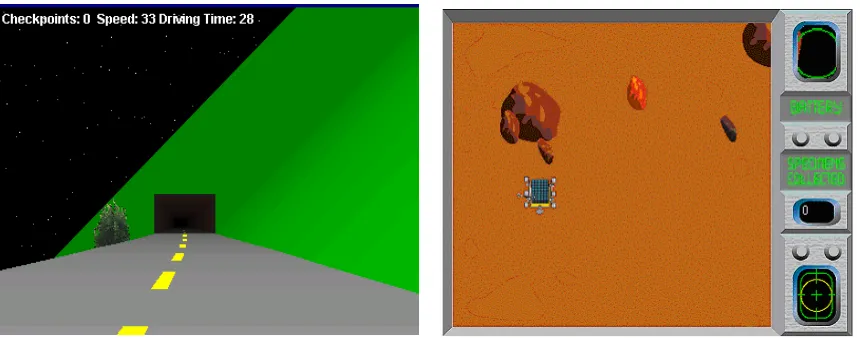
We have worked with two different games, whose interfaces are shown in Figure 1 and
Figure 2. All of these games were developed by others and have not been modified by
us. Figure 1 shows a first person driving game, in which the model controls the speed and
steering of the car. Figure 2 shows a Mars rover simulation. The goal is to direct the
rover over the planet surface, collecting as many specimens as possible. When the rover
collides with rocks, these disappear and release a small swarm of creatures to be chased
and captured. Although we have developed image-processing functions that can parse
both these environments, the only environment for which we have constructed complete
cognitive models is the driving game[9]. This game will thus be the focus of our
discussion.
As mentioned earlier, one of the targeted applications of this research is to provide a
means for evaluating the ease of use of a user interface. A human-robot interface is one
such interface that assumes much significance largely due to that fact that in the current
setting, robots are not fully autonomous and hence require supervision. The 3D-driver
game resembles a human-robot interface in several ways. On the surface level, it uses a
first-person view as task perspective and the environment changes dynamically in
response to the actions of the user and task environment, which is also the case for many
human-robot systems. On a deeper level, driving behavior is a prototypical example of
real-time, interactive decision making in an interactive environment. The simulation we
are using is comparable to many robot applications in that it relies heavily on
perceptual-motor skills, and involves decision-making under time pressure and interacting with a
dynamically changing environment. Furthermore, the driving game represents a
simplified driving environment, which corresponds sufficiently to real-life driving but is
nevertheless a controlled setting. Because its source code is extensible, we can
manipulate aspects of the environment (e.g., slow or fast driving) and add an interface
whose features can be varied (e.g., bigger or smaller buttons), essentially allowing for
3. Related Work
Our approach has been influenced by the work done in computer vision and image
processing systems dealing with object recognition. Object recognition is the process by
which the image-processing algorithm generates a symbolic representation of the
environment as required by the cognitive model. This process has been extensively
researched under the fields of computer vision and image processing. These are two
distinct but closely related fields falling under the umbrella of computer imaging. This
distinction is based upon who is the ultimate receiver of the visual information. Image
processing algorithms process images and the generated visual information is directly
used by human beings, whereas computer vision application processed images are used
by a computer[10]. Image analysis is an important topic in computer vision. Image
analysis combined with feature extraction and pattern classification is the key to a
computer vision system, the end product of which is the extraction of high level
information (such as objects) from an image. Most of the techniques used for image
processing are also used in computer vision systems.
In this section, we discuss the biological vision process and the three stages through
which it proceeds. Then, we describe the object recognition process in detail and its
correlation with human vision. We also explain some of the well-known
3.1 Visual Recognition in Humans
Because we are building cognitive models, the visual processing involved should ideally
be based on the model of biological vision. Another overriding objective of modeling a
vision system on human vision is that if the system is built the way the human vision
system works, then the vision system can be extended far more generally to different
domains than a system designed to work with specific image types. However, in practice,
even the most general-purpose systems have application specificity[11]. Below we
briefly describe the way biological vision works. Note that the terms biological vision
and human vision have been used interchangeably here.
Biological Vision
Vision is the process by which humans get an understanding of the world they live in.
Study of vision involves not only the way visual information is processed to produce a
description that is useful to the viewer, but also the way information is represented at
various stages of visual processing[12]. We are concerned with the former. Biological
vision proceeds in 3 main stages, which are
• Low Level Vision
• Intermediate Vision
During each of these stages, the visual image undergoes transformation from one
representation to another with each representation having more useful information than
the one in the preceding stage. It should however be noted that as we proceed from one
level to a higher level, some amount of information loss occurs. The boundary between
these 3 stages is a blurred one.
3.1.1 Low Level Vision
Low level vision refers to the visual processes responsible for generating representations
that give information about the properties of the surrounding environment. These
processes do not need knowledge about the domain in which they operate and do not
need to recall memories about the objects already seen and known. They operate directly
on the visual stimulus regardless of the task being performed. They rely on the physical
properties of objects such as continuity and rigidity. Different parts of this visual field
can be processed at the same time, and hence low level vision processes are bottom up
and parallel (spatially uniform). Some such processes are those that analyze movement,
surface shading, texture and color.
A dominant visual process during low-level vision is edge detection. An image, as
captured by the photoreceptors of the eyes, can be thought of as forming a very large 2D
array of light intensities. Experiments in animals have revealed that images are usually
treated as equivalent to a sketch of their outlines. Even in humans, perception of an image
Binocular stereo and analysis of visual motion[13] are other dominant visual processes
occurring during this stage of vision.
Marr, in his analysis of vision, describes a representational framework for the early visual
processes that constitute low level vision[14]. He points out an important characteristic of
human vision that it tells about shape and space and spatial arrangement. This implies
that even in absence of information about objects, it is possible to correctly perceive the
geometry of objects.
The suggested framework consists of three representational stages.
• Representation of properties of the two dimensional image, such as significant
intensity changes and local 2D geometry. This involves operations such as edge
detection, peak finding and zero crossings.
• Representation of properties of the visible surfaces in a viewer-centered coordinate
system, such as surface orientation, distance from the viewer and some coarse
description of prevailing illumination. This involves operations such as binocular
stereo.
• Representation of the 3D structure from an object-centered coordinate system and its
3.1.2 Intermediate Level Vision
Intermediate level vision refers to the visual processes that are concerned with grouping
entities together. There is a thin line between intermediate and high level vision. The
difference lies in the fact that processing that falls under the realm of intermediate vision
does not require knowledge of the properties of specific objects in the world. However, it
is still dependent on the task being performed[15]. The term intermediate vision does not
necessarily imply the order in which the processing phases itself; it is possible that high
level processes are executed without relying on intermediate level processes.
Processes that extract shapes and analyze their spatial relationship usually constitute
intermediate vision. Which shapes to extract is a task dependent problem. In order to
examine the spatial relationship, the visual processes cannot operate on separate parts of
the visual field independently. Hence, intermediate level vision has properties of
non-uniformity and open-endedness[13].
3.1.3 High Level Vision
High level vision refers to the visual processes that help in carrying out tasks such as
visual object recognition, visually guided manipulation, locomotion and navigation
through the environment. These processes are heavily dependent on the task being
performed, and rely on knowledge about the properties of objects such as their shape,
catalog of objects in the long-term memory and comparing the representation of various
objects within this catalog with the representations of objects that have been generated
during the preceding stages[13]. Thus, it is more a problem of memory organization,
retrieval and reasoning.
3.2 Image Processing for Object Recognition
As will be seen, the object recognition process exhibits a moderate level of similarity
with the human visual recognition process. The object recognition process (as a part of
image analysis) can be viewed as a sequence of the following steps[10].
• Preprocessing the image
• Data Reduction and Morphological filtering
• Feature extraction and analysis
Any image processing or computer vision algorithm that deals with automatic object
recognition, in order to be robust, should consider the effects of
• Non-uniform lighting
• Occlusion (of one object by another)
• RST (rotation, scalability and translation) characteristics of an object
• Object deformities (i.e. partial defects in object)
The design itself should be such that the problems caused by these factors do not have a
telling effect on the ultimate performance of the algorithm[16].
3.2.1 Preprocessing
During this stage, the image may be quantized (reducing the number of color levels or
spatially) or it may be enhanced to prepare it for the subsequent processing steps. Some
other image geometry operations such as crop, zoom, shrink, enlarge, translate and rotate
may be performed on the entire image or parts of image (called regions of interest). Much
of the work done during this phase of object recognition process constitutes part of what
is done during the early vision phase in humans[11].
Another important and widely used preprocessing operation is edge detection. Edge
detection is a procedure that finds the borders of objects in an image and thereby,
indirectly extracts them. It is a group operation since it looks at the values of the
neighboring pixels. It is often used as an intermediary step in more sophisticated
segmentation algorithms and frequently as the preliminary step to the line detection
process. The most common edge detection method is a gradient-based procedure that
calculates the gradient and uses a gradient threshold to determine the presence of edge.
These methods are basically discrete approximations to the differential methods, which
identify an edge as a large change in color/texture over a small spatial distance.
Typically, a mathematical process called convolution is used for this purpose. A
additional rows and columns. The mask is overlaid on the image and the coincident
values are multiplied and the results are summed up to get the new pixel value at the
image location corresponding to the center of mask. Different types of kernels may be
used for edge detection. These kernels can be directional or non-directional. Once the
edges have been detected, it may be necessary to find out lines. A line may be defined as
a collection of edge points that are adjacent and have the same direction. Hough
transform[17] is often used for this purpose and is described later.
3.2.2 Data Reduction & Morphological Filtering
The data reduction algorithms take the preprocessed image and reduce the image data
such that it can be analyzed by feature analyzing algorithms. This is a crucial step to the
object recognition problem and involves image segmentation as the key to it.
Morphological filtering refers to changing the structure/form of the image. This phase
also contributes to the processing occurring during the early vision stage.
Segmentation is the process of delineating regions that constitute an object and separating
them from the background in an image. It is directly influenced by the category to which
the game belongs. The goal of image segmentation is to divide the image into regions,
which may represent an object in its entirety or may be part of a larger object. Various
methods exist to segment an image into regions with varying levels of complexity and the
accuracy with which the image is segmented. The basic idea underlying these methods is
with some measure of homogeneity in terms of features such as color, brightness, texture
or perceiving them as having contrast with other objects on their borders. Another
important issue is related to connectivity between segments i.e. deciding the segments
that should be combined so that they represent an object. For this purpose, neighboring
pixels are examined. A pixel has a maximum of 8 neighbors. The connectivity can be
determined by examining either of the following.
• 8 neighboring pixels (eight connectivity)
• 4 neighboring pixels: north, east, west and south (four connectivity)
• 6 neighboring pixels: north, east, west, south, northwest and southeast (six
connectivity NW/SE) or north, east, west, south, northeast and southwest (six
connectivity NE/SW)
Most of the image segmentation algorithms make use of one or more of the below
mentioned techniques.
• Region growing and shrinking
• Clustering
3.2.2.1 Image Segmentation techniques
Region growing and shrinking
This refers to the class of methods that process the image in essentially the spatial
domain. Initially, the image is split up into a fixed number of regions. This region can be
the entire region itself or it may be a single pixel (making the number of regions equal to
the image resolution) or this initial number can be chosen based on some other criterion.
Once the initial partition is done, these regions are then merged or split. Three important
notions taken into account during this merge/split are merge order, merge criterion and
region model[18]. Merge order defines the order in which the regions should be merged.
Given two regions, merge criterion is used in determining whether they should be merged
or not. This merge criterion is usually some kind of homogeneity test and it is largely
application dependent. Region model defines the representation of the resulting merged
region.
This technique of image segmentation gives rise to a hierarchically segmented image,
where, at different levels in the hierarchy, the image is segmented at different levels in
terms of the fineness of segmentation. The merge/split is recursively performed until a
specified criterion is met (for example, all the regions pass the homogeneity test or the
image is factored into a pre-defined number of regions). There are many variations of this
Clustering
This refers to the class of methods that use domains other than the spatial domain as the
primary domain for clustering. Some such domains include color space, histogram space
and feature spaces. Histogram thresholding[19], which is explained later, is one such
method.
Boundary Detection
This refers to the class of methods that detect objects by finding boundaries between
objects. These boundaries indirectly segment the image into objects. The normal
procedure followed here is to edge detect the image, and then combine these edges into
line segments, which, then are merged into object boundaries.
3.2.2.2 Segmentation Algorithms used in practice
Some of the segmentation methods that have been used in practice are explained below in
non-decreasing order of their complexity.
Thresholding
This is one of the simplest segmentation techniques[19] and belongs to the class of
algorithms based on the clustering technique described earlier. A threshold (θ) is chosen
and all the pixel values above (or below) that threshold are set to 0. This implies that
those pixels that are set to zero comprise the background. This can be stated in
For bright object on dark background,
if brightness (pixel(x,y) ) >= θ
brightness (pixel(x,y)) = 1
else brightness (pixel(x,y)) = 0
For dark object on light background,
if brightness (pixel(x,y) ) < θ
brightness (pixel(x,y)) = 1
else brightness(pixel(x,y)) = 0
The thresholding parameter can also be something other than the brightness. For
example, in a RGB image, each of the R, G and B bands may be checked against
different thresholds. The important decision in thresholding is choosing the threshold
value. Some of the common techniques for determining this value are described below.
Fixed threshold
This is the simplest of all methods of choosing the threshold. Here, the threshold value is
chosen independently of the image data. This method is useful for those images in which
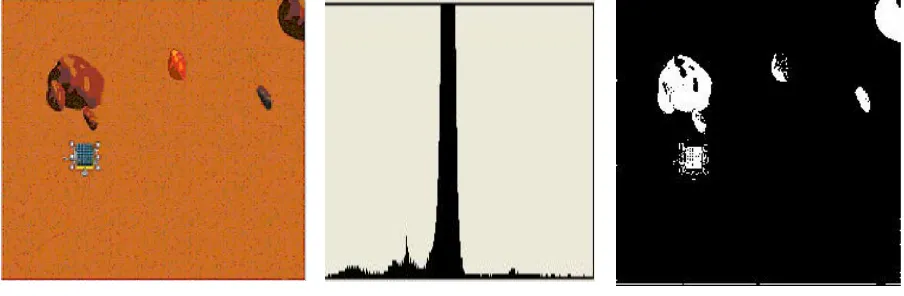
the background is homogenous and in contrast with the foreground. Consider Figure 3
Figure 5 show the histogram (color intensity on X-axis and number of pixels on Y-axis)
and the thresholding operation on it with a threshold value of 94 respectively.
Figure 3. Original Image Figure 4. Histogram Figure 5. Thresholding (θ = 94)
Histogram derived threshold
Other techniques for determining the threshold make use of the histogram of the image
pixel values. The histogram may be smoothed to reduce the effect of small fluctuations.
Some of the algorithms that use the histogram to find the threshold value are listed below.
• Isodata algorithm
This is an iterative method to determine the threshold. Initially, the threshold is chosen as
the mid-value of the range of pixel values. Then, mean values of the pixels on both sides
of that threshold are computed and their mean is found. This procedure is repeated until
This can be represented as
θ (i) = (θ (f,k-1) + θ (b,k-1) )/2 until
θ (i) = θ (i-1)
• Triangle algorithm
This method is useful when the histogram doesn’t have a distinct peak. A line connecting
the peak in the histogram and the least pixel value in the image is drawn, and the distance
of this line from the histogram is computed at each pixel value. The threshold is the pixel
value where this distance is maximum.
• Background symmetry algorithm
This method is useful when the histogram has a strong and distinct peak. The peak value
in the histogram is found, and a p% value is computed on the non-object side of the
histogram. The threshold is then chosen as below.
θ = peak_pixel_value – (p% value –peak_pixel_value)
The p% value indicates that only (1-p) percent of pixels have a value greater than the p%
Region Growing Using Recursive Shortest Spanning Tree and Binary Partition Tree
This technique of image segmentation falls under the genre of region growing algorithms.
It is a bottom-up method that starts out by viewing the image as a graph and each pixel in
the image as the node of the graph. The nodes in the graph represent the regions found so
far. Thus, the initial number of regions is equal to the number of pixels in the image.
Each region in the initial graph is connected to its four adjacent regions via a link. The
cost of this link is calculated as a function of luminance, chrominance and area values
between the two adjacent regions. This cost represents the distance between the two
regions. The lower this cost, the more likely that these two regions belong to the same
segment (and hence the object). The area of region here indicates the number of pixels in
that region. Thus, the distance is calculated as
(
)
{
[
]
[
] [
]
}
) ( ) ( ) ( ) ( ) ( ) ( ) ( ) ( ) ( ) (, 2 2 2
Rj N R N Rj N R N Rj V R V Rj U R U Rj Y R Y Rj R d i i i i i i + × × − + − + − = ,
where Y, U and V indicate the three different streams in YCbCr color space and N
indicates the number of pixels belonging to that region[18].
The two regions that have the minimum distance between these are merged together into
a single region and the mean value of the chrominance and luminance is calculated that
now represent the chrominance and luminance of the merged region. The new area is also
calculated and the link between the two regions is removed, thereby forming a spanning
tree of the graph. This process is repeated over and over again until the image is
hierarchically segmented image, where the image coarseness increases down the
hierarchy.
Often, the segmented image obtained using the above method is subjected to some further
processing to extract the object. One such technique is called the Binary Partition Tree
method. It starts with a given initial partition and the regions in this initial partition form
the leaves of the tree. These regions are then merged in the order specified by merged
order (defined earlier) according to a merge criterion. The merging continues until one
single region is obtained. The resulting binary tree represents the image at different scales
of resolution.
3.2.3 Feature Extraction and Analysis
This phase is comparable to the intermediate level and the high level processing stages in
human visual processing system. Feature extraction phase corresponds to the
intermediate level processing (though there are some distinctions between the two in that
feature extraction is often driven by information about specific objects). Shape detection
is an important part of the feature extraction process.
Care should be taken while selecting the features, so as to ensure that the features chosen
are robust. A feature if RST invariant (rotation, scaling and translation invariant) will
In order to extract features, the image that results from data reduction and morphological
filtering is analyzed and labels are then assigned to the objects. The labeled object now
can be thought of as a binary image having a value of 1 and the rest of the image is
having a value of zero. This image is then used to extract features of interest such as area,
center of area, axis of least second moment, perimeter, Euler number (defined as the
number of objects minus the number of holes) , projections, thinness ration and aspect
ratio[10]. While the first four are used more commonly and help identifying the location
of the object, the latter four are used under specific conditions and tell something about
the shape of the object. The way they are obtained is explained below.
Let Ii at a given location (x,y) be defined as
if (x,y) belongs to ith object,
Ii(x,y) = 1,
else
Ii = 0
So, the area is now defined as
Ai =
∑
∑
− = − = 1 0 1 0 ) , ( N x i N y y x I
And the center of this area is given by
i
y =
i
A
1
∑
∑
−= − = 1 0 1 0 ) , ( N x i N y y x yI
The axis of least second moment gives information about object’s orientation. This axis is
the axis about which it takes the least amount of energy to rotate the object. It is
calculated as
tan(2θi) = 2
∑
∑
∑
∑
∑
∑
− = − = − = − = − = − = − 1 0 2 1 0 1 0 2 1 0 1 0 1 0 ) , ( ) , ( ) , ( N x i N y N x i N y N x i N y y x I x y x I y y x xyIThe perimeter P is calculated by adding up all the ‘1’ pixels that have a ‘0’ pixel as
neighbor. The other method is to find the edge of the object and then calculate the
number of ‘1’ pixels.
The thinness ratio T is calculated as
T = 4п 2 P A
T = 1 indicates that the object is a circle. As the value of T decreases, the object increases
in thinness. The inverse of thinness ratio is called the irregularity or compactness ratio.
The Euler number is used for optical character recognition and it is defined as the number
of objects minus the number of holes (for example, the Euler number of the character ‘o’
Projections are also used in applications like character recognition. Moreover, for optical
character recognition, a method that takes projections on horizontal and vertical planes
can also be used.
The horizontal projection is calculated as
hi(y) =
∑
− = 1 0 ) , ( N x
i x y
I
The vertical projection is calculated as
vi(x) =
∑
− = 1 0 ) , ( N y i y x I
Often, it is necessary to derive information about the shapes present in the image. Hough
transform is the ideal candidate for this purpose.
3.2.3.1 Hough Transform
Hough Transform is a proven tool for detecting simple shape primitives such as line,
circle, ellipse, parabola and the like. It can also be used to detect general shapes. The
characteristic of Hough Transform that makes it an attractive choice for shape detection
is its ability to work well on images that have been distorted by noise. It also works well
for locating objects that have been occluded by some other objects or when the
preprocessing stages (usually some type of edge detection) yield an under detected
However, Hough Transform per se is computationally prohibitively expensive and this
has been the major stumbling block retarding its wide spread use. Another factor working
to its disadvantage is the storage requirement as imposed by this algorithm. Techniques
have been devised that have made this algorithm practically possible to implement,
though under some constraints[16].
The classical Hough transform can identify those shapes that can be described in terms of
parameters. Generalized Hough transform can be used to detect those shapes that do not
have a parametric description. Hough Transform usually takes as input an image that has
been edge detected and works on the resulting set of edge points.
The principal idea underlying Hough Transform is that each shape that is required to be
detected from a given set of edge points in spatial domain can be described in terms of
parametric equation and that each of the edge points contributes to a subset of the entire
parameter space with the property that the target shape’s parameters will correspond to
the intersection of the subsets formed by the edge points. If a shape is described by 3
parameters, then the parameter space will be 3 dimensional. An accumulator array is
defined over the parameter space that keeps a track of the number of points in spatial
domain that contribute to this point in the parameter space. The bin in this accumulator
array that contains the highest number of edge points identifies the parameters, which
best fit, the shape in question. A threshold can also be used so that all the bins in the
accumulator array which have value greater than this threshold are chosen for further
with an increase in the dimensionality of the parameter space. Also, the time required in
looking at each bin in the accumulator array will increase. This makes this method very
expensive in terms of computational time and storage requirements.
One of the variations of Hough transform that tries to address this problem divides the
parameter space into regions (i.e. the parameter space is quantized). The accuracy of
Hough Transform algorithm is however compromised (for example, 2 lines lying close to
each other, would be mapped to the same block in parameter space). Nevertheless, it is
effective in reducing the storage space requirements as well as the computation time. The
quantization blocks themselves can vary in size and the advantage of having large such
blocks is that the search time and storage requirements decrease.
Line Detection using Hough Transform
Line is a collection of adjacent edge points having same direction. The parametric
equation of a line that Hough Transform makes use of is
xcosθ + ysinθ = ρ,
where ρ is the distance of the foot of perpendicular from the
origin. Thus, the parameter space is 2 dimensional, ρ and θ
being the parameters. For each edge point in spatial domain, the value of ρ is calculated
parameter space. At the end of this process, the number of hits in each block indicates the
number of edge points that lie on the line(s) described by this block. Depending upon the
threshold, a decision is made as to which lines exist in the image.
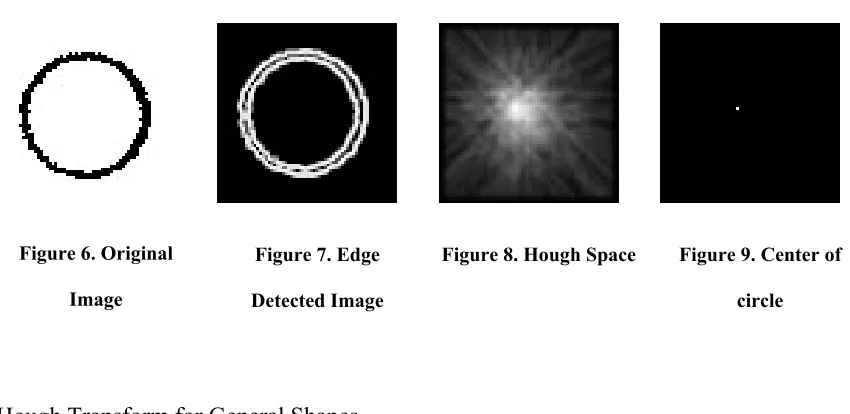
Circle Detection using Hough Transform
The parametric equation of circle used by this method is
(x –a) 2 + (y-b) 2 = R2, where (a,b) is the center of the circle and R is its radius.
Given as set of edge points, the objective is to find the center of the circle on which the
points lie. This assumes that the radius of the
circle is known in advance and that each edge
point is on the boundary of the circle. For each
edge point in the edge-detected image, a
candidate center point is obtained which lies at a
distance R in the direction of normal to the local
edge. This produces a set of candidate center
points in the parameter space. The points are accumulated in the accumulator array and
the center of circle is the block in this array that has the peak value. As it can be seen
from this method, even in the case of partially occluded objects, the peak point found in
the parameter space still will be the actual center of the circular object and hence this
method works well. However, a lot of storage space is required for the accumulator array.
In addition, relaxing the constraint that the radius is known in advance, the method will
have to compute the values for accumulator array for every different possible radius
value and this can be seen as employing different planes in the parameter space, one for
each radius value. However, prior knowledge of gradient (obtained using a directional
edge detection filter) can help in speeding up this process. Extending the gradient vectors
at each edge point within the image space can achieve this. All gradient vectors will
intersect at the point that marks the center of the circle. The following figures show the
output of Hough transform applied to a sample circle.
Figure 6. Original Image
Figure 7. Edge Detected Image
Figure 8. Hough Space Figure 9. Center of circle
Hough Transform for General Shapes
The Hough Transform is computationally very expensive when used to locate general
shapes whose orientation is unknown[20]. When it is known, however, it is possible to
get away with a single plane in the parametric space. To improve the efficiency when
dealing with special cases like ellipse and polygons, separate solutions have been
Once the features have been extracted, the next step is to classify them to identify objects.
This requires application level knowledge and hence, application specific knowledge is
used in this final phase. This corresponds to the high level vision processing occurring in
human visual system. One way to classify objects is to define a feature space and then
compare the object’s feature vector against the actual object’s feature vector. A feature
vector is an n-dimensional vector such that each dimension represents exactly one feature
of the object. Thus, for example, if three separate features characterize an object, then the
corresponding feature space is three-dimensional. Different methods are used to compare
the similarity (or the difference) between two feature vectors. The most common metric
used to measure the distance between two vectors is the Euclidean distance between
them. For two vectors X = [x1,x2,…,xn] and Y = [y1,y2,….,yn], the Euclidean distance
between X and Y is defined as
2 2
2 ( 2 2) ... ( )
) 1 1
(x −y + x −y + + xn−yn
A variation of this basic Euclidean distance called range-normalized Euclidean distance
is sometimes used to account for large differences between the corresponding
components of the two vectors being compared.
Another metric used for comparing two feature vectors that uses the similarity measure is
the vector inner product. For two vectors X and Y as defined above, it is defined as
(x1.y1 + x2.y2 + …..+ xn.yn)
4. The System
We have made an attempt to design our image processing algorithms based on the model
of biological vision. At the same time, we have considered other efficient means of
solving the same problem, and described the tradeoffs of using these two different
approaches. The efficient approach is an engineering approach to the visual image
analysis problem. Our approach to image processing reflects a combination of these two
approaches.
In this section, we describe the overall system architecture and its components. We first
describe the core vision system and all the operations it provides with a pseudo code of
their procedure. Then, we describe image-processing approach taken for the two games.
For each game, we discuss the cognitive model requirements, the image-processing
operations, the underlying assumptions, the rationale behind the approach and its
limitations.
4.1 System Design
Figure 10 shows the generic architecture of the system that involves a cognitive model
interacting with image processing substrate to get information (in symbolic form) about
Figure 10. Architectural Diagram of the System
We have developed a cognitive model only for the driving game. This model is based on
the ACT-R architecture. It gets information about the environment from the image
processing substrate and takes action using the mouse and keyboard input functionality
provided by SegMan. The image processing substrate takes pixel-level input from the
screen (i.e., the screen bitmap) by capturing snapshots of it at regular intervals. For this, it
makes use of APIs provided by the SegMan system. Thus, SegMan provides sensor and
effector services to the system.
As can be seen, the image processing substrate consists of a generic core vision
subsystem and an application specific sublayer on top of it. The generic core provides
The application specific sublayer consists of functions that provide a general level of
information about the image. Because tasks inevitably have domain-specific properties,
we must tailor the image-processing component by adding functions for specific games.
For the driving game, the extensions are based on studies of human driving as will be
explained later. These additional functions are built on the generic core.
4.1.2 Generic Core
The generic core is intended to provide much of the functionality that is seen during the
early stages of vision. The functions that it provides can be used directly on the captured
image to preprocess it. They could also be called from within the application specific
layer for application specific processing.
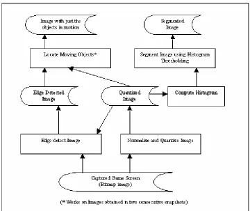
Figure 11 shows the control flow within the generic core. The operations such as edge
detection could either work directly on the captured image or the normalized and
quantized image. Normalization and quantization is always performed on the captured
image. Histogram is computed from the normalized and quantized image. This histogram
is subsequently used by the segmentation algorithm to determine the threshold based on
which it segments the normalized and quantized image. For locating moving objects,
Figure 11. Control flow Diagram of Generic Core
The following operations are currently supported in our core vision system.
Normalize and Quantize Image.
Usually the captured image contains a level of detail (in terms of number of values in
the R, G and B streams in the image) not needed to serve the model's purpose of
controlling the game effectively. This function normalizes the number of color levels
Quantization is specified in terms of the number of levels desired in each stream. A
value of x for each level means x Red levels, x Green levels and x Blue levels,
resulting in a total of x^3 colors. It has been found that with three quantization levels,
most of the necessary information is maintained.
It should be noted that knowledge of the domain influences the choosing of certain
parameters (such as number of quantization levels or the shape of object to look for)
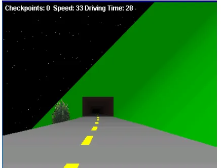
used during the first two phases. Figure 13 shows the effect of applying this operation
to a snapshot of the 3D-Driver game.
For each pixel in the image - Read the pixel color value
- Get the R, G and B components of the color value
Split the range 0-1 into a number of intervals equal to the number of levels desired minus one
For each interval, find the mid-value of that interval. Thus, a level will represent all the values that lie between the mid-value belonging to the previous interval and the mid-value belonging to the next interval
Accordingly, determine which level in 0-1 do normalized R, G and B values computed earlier belong.
Scale the normalized value back to the desired level in range 0-1
Determine the value of resultant R, G and B values in the range 0-maximum value that R, G and B can have
Combine the quantized R, G and B values to get the resultant pixel value
Figure 12. Driving environment without any image processing
Figure 13. Driving environment after normalization and quantization
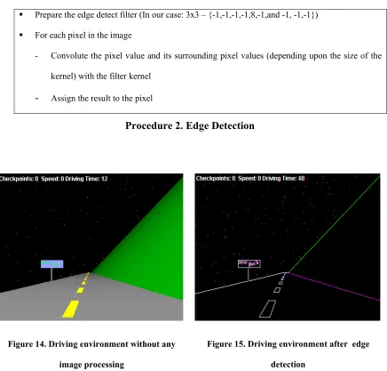
Edge Detect Image.
This function highlights changes in color intensity values in the image. Laplacian 3x3
edge detection kernel is used for convolution. This kernel, shown below is
non-directional. − − − − − − − − 1 1 1 1 8 1 1 1 1
A convolution operation of the image pixel values is performed with the kernel.
Figure 15 shows the effect of applying this operation to a snapshot of the 3D-Driver
Prepare the edge detect filter (In our case: 3x3 – {-1,-1,-1,-1,8,-1,and -1, -1,-1})
For each pixel in the image
- Convolute the pixel value and its surrounding pixel values (depending upon the size of the kernel) with the filter kernel
- Assign the result to the pixel
Procedure 2. Edge Detection
Figure 14. Driving environment without any image processing
Figure 15. Driving environment after edge detection
Compute Histogram.
This function computers the histogram of the normalized and quantized image. The
histogram is used for the selection of a threshold in the subsequent segmentation
Create a hash table which uses color intensity value as the key
Scan the image from left to right and top to bottom
At each location, get pixel color value
If pixel value already a key in hash table
- Increment the count associated with that key
Else
- Create a new entry in hash table with the pixel value as the key - Initialize count to 1
Find the key with the maximum count in the hash table. This key represents the peak in the histogram and corresponds to the color intensity occurring most frequently in the image.
Procedure 3. Compute Histogram
Segment Image using Histogram Thresholding.
This function segments the image using the threshold value computed using the
histogram. It basically separates the foreground objects from the background.
Use the computed histogram and determine the peak pixel value corresponding to the background intensity using the peak finding test. Put thresholds on either side of this peak.
Scan the image from left to right and top to bottom
At each location, get pixel color value
- If pixel value within the two thresholds, it represents a background pixel - Mark this value zero
Locate Moving Objects.
This function detects moving objects in successive game screen snapshots. It
assumes that the background remains static and the only change in the environment is
due to moving objects. The two edge detected images (say image1 and image2)
obtained during the earlier processing step are ORed with each other which yields an
image that shows the new position of the object superimposed on the image1. The
rationale behind using OR operation is that except for the moving objects, everything
else in the two consecutive images would remain same. Subtracting image1 from this
ORed image will give the object that is moving.
Capture two snaps of the environment. Call them image 1 and image 2
Edge detect image1 and image2 using Procedure 2
OR image1 and image2
Subtract image 1 from the resultant image2
Procedure 5. Locate Moving Objects
4.2 Mars Rover
Figure 17 shows one snapshot of the environment in Mars Rover game. The game
environment is relatively static, predictable, simple (classification of objects based on
color and motion) and crowded. Usually, the environment changes only upon the some
action from the model. However, for some time after that, the environment keeps on
changing by itself, after which it again becomes static. The number of objects (here rover
and rocks) can be large and hence it is crowded.
Figure 16. Screen capture of Mars Rover
4.2.1 Cognitive Model Requirements
To achieve the objective of this game, the information that a cognitive model needs is
information about the current position of the rover (relative to some axes), position of the
rocks and the position of the creatures that are released upon collision with a rock.
4.2.2 Approach
A two-stage segmentation approach has been used. The first stage performs a coarse
segmentation based on histogram thresholding as described in section 3.2.2.2. The