ABSTRACT
BAKIR, ILKE. Linear Programming Formulations for Production Planning Problems with
Alternative Routings. (Under the direction of Dr. Reha Uzsoy).
Linear programming (LP) is a common tool for solving production planning
problems. However, LP formulations tend to get very large, when used for modeling
large and complex production systems, such as production systems with alternative
routings. In this thesis, we define production planning problems with alternative
routings, investigate different modeling approaches to such problems, and propose a
solution method.
We first present the “Path Based Formulation”, which grows rapidly in terms of
number of variables. Then we propose a Column Generation formulation to solve the
path-based problem more efficiently, without generating all variables corresponding to
the alternative routings. We also present some compact LP formulations, which are
used for modeling production planning problems with alternative routings, from
existing literature; namely “Direct Product Mix Formulation” of Leachman and Carmon
(1992) and “Capacity Partition Approach” of Hung and Cheng (2001).
Linear Programming Formulations for Production Planning
Problems with Alternative Routings
by
İlke Bakır
A thesis submitted to the Graduate Faculty of
North Carolina State University
in partial fulfillment of the
requirements for the Degree of
Master of Science
Industrial Engineering
Raleigh, North Carolina
2011
APPROVED BY:
_______________________________
______________________________
Dr. Reha Uzsoy
Dr. Thom J. Hodgson
Committee Chair
_______________________________
DEDICATION
BIOGRAPHY
ACKNOWLEDGMENTS
I would like to sincerely thank my advisor, Dr. Reha Uzsoy, a million times for
making this thesis possible by guiding me through my research, constantly supporting
me in all the problems I face, and patiently tolerating my reactions to tough situations,
especially towards the end. He has been not only an academic advisor, but also a
mentor and a counselor to me. I also would like to thank the members of my advisory
committee, Dr. Thom J. Hodgson and Dr. Brian Denton for taking the time to serve in my
committee, review and critique my thesis.
I am grateful to the faculty and staff of Edward P. Fitts Department of Industrial
Engineering for giving me the opportunity to initiate my graduate studies, providing me
with an academic “home” for my research activities, and give me the knowledge basis
necessary to continue my studies.
TABLE OF CONTENTS
LIST OF TABLES _______________________________________________________________________________ vi
LIST OF FIGURES _____________________________________________________________________________ vii
1.
Introduction _________________________________________________________________________________ 1
2.
Problem Definition and Formulations ____________________________________________________ 7
A.
Problem Definition ____________________________________________________________________ 7
B.
Path-Based Formulation ______________________________________________________________ 8
C.
Column Generation Formulation for Path-Based Model _________________________ 11
D. Direct Product Mix Formulation ___________________________________________________ 19
E.
Capacity Partition Approach ________________________________________________________ 25
3.
Design of Experiments ___________________________________________________________________ 31
4.
Computational Results ___________________________________________________________________ 33
A.
Proportion of Generated and Used Columns ______________________________________ 33
B.
Solution Times of CG, and Comparison with PB __________________________________ 36
C.
The Effect of Process Time Variability, Lead Time Variability, and Machine
LIST OF TABLES
Table 2.1: Data for CSGP Example ___________________________________________________________ 21
Table 2.2: Outcome of CSGP Example _______________________________________________________ 21
Table 2.3: Data for CPGP Example ___________________________________________________________ 27
Table 2.4: Outcome of CPGP Example _______________________________________________________ 27
Table 3.1: Design of Experiments with Different Values of Parameters _________________ 32
Table 4.1: Proportion of Generated Columns vs. Number of Possible Paths _____________ 34
Table 4.2: Proportion of Used Columns vs. Number of Possible Paths ___________________ 35
Table 4.3: Hypothesis Testing for the Difference of Means (Low Process Time Variability
vs. High Process Time Variability) __________________________________________________ 43
Table 4.4: Hypothesis Testing for the Difference of Means (Lead Time Variability vs. No
Lead Time Variability) _______________________________________________________________ 45
Table 4.5: Hypothesis Testing for the Difference of Means (Low Machine Utilization vs.
LIST OF FIGURES
Figure 1.1: Path-Based Formulation of Alternative Resources _____________________________ 2
Figure 2.1: Representation of Two Nodes and an Arc in the Subproblem Network _____ 17
Figure 2.2: The Directed Graph G=(N,A) Defining the Column Generation Subproblem
_________________________________________________________________________________________ 18
Figure 2.3: Network Representation for Capacity Constraints of Direct Product Mix
Formulation ___________________________________________________________________________ 24
Figure 2.4: Capacity Partitions for CPGP Example _________________________________________ 27
Figure 4.1: Proportion of Generated Columns with Changing Problem Size _____________ 33
Figure 4.2: Proportion of Generated Columns with Changing Number of Possible Paths
1.
Introduction
Linear programming (LP) is widely used for solving a wide range of production planning problems. However, LP formulations can get very large, especially with large and complex production systems such as those encountered in semiconductor manufacturing; hence the challenge has always been finding the most compact model possible while still achieving the desired level of accuracy. In particular, production planning problems where products can be produced using different combinations of flexible resources have proven particularly difficult to model.
There are many different production planning models available in the literature; both for deterministic and stochastic demand structures (Johnson and Montgomery, 1974). This thesis focuses on deterministic production planning problems with alternative machine types. The production planning models considered in this research aim at determining an optimal, capacity-feasible product mix for each planning period over some planning horizon in a production facility with following characteristics:
- Multiple production stages
- Alternative machine types, i.e. machine types that are functionally different but capable of performing the same manufacturing operation, at each stage, perhaps at different quality levels and with different processing times
- Discrete time periods - Single commodity
The particular production system we will consider within the scope of this thesis has multiple stages and multiple machines at each stage. All the machines at each stage are capable of performing the same operation on the product. It can thus be classified as a flexible flow shop structure. Although the models we develop can be extended to more complex production systems, such as those with reentrant product flows, we focus on the flexible flow shop environment due to the ease of controlling the number of alternative paths through the system, which simplifies the design of our computational experiments.
sequences of operations that can produce a product, grows exponentially with increasing number of stages. These formulations provide detailed information on the workload assigned to each machine or the proportion of jobs that use a particular machine type in each planning period. The purpose of the planning process, however, is finding a capacity-feasible job release schedule that specifies the amounts of the product to be released into the production system in each time period while satisfying the demand constraints.
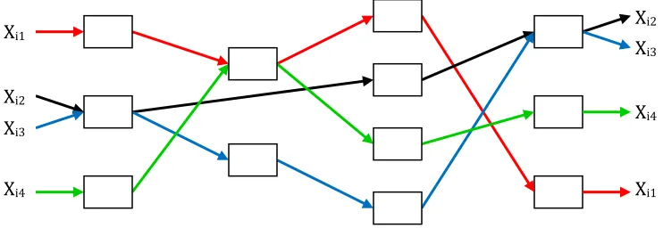
Path-based formulations are mathematical models that keep track of how much work is allocated to each possible sequence of operations. These are called Path-Based formulations, since we are explicitly specifying the amount of each product that will be launched on each possible path through the production system in each period. Such a formulation is depicted in Figure 1.1, which represents a production system with four stages with a number of alternative machines at each stage, represented by the boxes. Path-Based formulations, referred to as Process Selection Models by Johnson and Montgomery (1974), have been known for quite some time, but have the obvious drawback that in a production system of any complexity, the number of possible paths through the system that a product can follow, and hence the number of decision variables in a time period, grows exponentially in the number of alternatives at each stage and the number of stages. It is a fact that Path-Based formulations can be very flexible in the sense that they can be used to model almost any production environment; but their flexibility comes at a cost of significant computational complexity resulting from the necessity to generate all possible paths in advance and assign a variable to each path for each period.
Figure 1.1: Path-Based Formulation of Alternative Resources
The concept of the path-based formulation immediately suggests an approach where paths are generated as they are needed, and do not all have to be generated a priori resulting in an exponentially large LP formulation. Column generation approaches based on Dantzig-Wolfe decomposition (Bertsimas and Tsitsiklis, 1997) and similar approaches have been used to solve
Xi1
Xi2
Xi3
Xi4
Xi2
Xi3
Xi4
large problems in many areas. One of the early examples of the method is the method used by Ford and Fulkerson (1958) in their paper on maximal flow problems on multi-commodity networks. They state that solving such problems by Simplex Method would not be possible with available machine capacity, so they suggest performing the “pricing” operation of Simplex Method (i.e. the determination of a vector to enter the basis) implicitly. They show that finding the entering variable that would improve objective value the most is equivalent to solving a shortest chain problem. They also show that the shortest chain problem can be reduced to a standard transshipment problem, which may be solved in various simple ways.
Tomlin (1966), in his paper on minimum cost multi-commodity network flows, shows that such problems can be solved by a technique similar to the method proposed by Ford and Fulkerson (1958); i.e. determining the entering variable by solving a subproblem that obtains the column whose introduction to the basis would improve the objective value the most, while satisfying the feasibility constraints. In this case, subproblems have the form of a minimum cost flow problem in an uncapacitated network, and such problems can easily be solved using one of the efficient shortest chain algorithms (Ahuja, 1956 and Bazaara, 2010).
The column generation approach of Ford and Fulkerson (1958) has been extended and used for solving multi-commodity network flow problems by Folie and Tiffin (1976), Farvolden, Powell, and Lustig (1993), Barnhart et al. (1995), Desaulniers et al. (1997), Venkatadri et al. (2006), and Alvelos and Carvalho (2007).
The paper by Alvelos and Carvalho (2007) extends the type of work pioneered by Ford and Fulkerson (1958) by defining a new model and proposing a column generation approach to the minimal cost multi-commodity flow problem. Their extended model incorporates some additional variables, converts some simple constraints into ranged constraints, and requires an additional procedure to give an optimal solution to the original problem. Even though their extended model has more variables and more complex constraints, it has the advantage of reducing the number of iterations it takes for the column generation approach to solve the problem, and their experimentation show that the column generation approach implemented on the extended model improves the solution times greatly.
a production environment with continuous processes. Jain and Palekar (2005) indicate that their Configuration-Based model, which considers process and setup times of each machine configuration, i.e. path, separately allows them to overcome the limitations of Resource-Based models, which represent the workload on machines independently from the process path being used. Even though the Configuration-Based model increases accuracy significantly, it also increases the problem size in terms of number of variables and number of constraints. The authors also present some heuristics to limit the number of variables and show that they are effective in solving real-life problems.
Along with Path-Based approaches, there are also alternative formulations for the production planning problem. A number of authors have proposed more compact formulations of the problem with reduced numbers of decision variables and constraints. Leachman and Carmon (1992) propose three alternative production planning formulations that are often, although not always, more compact than conventional path-based models that accommodate alternative machine types. These models aggregate the capacity constraints to eliminate unnecessary details, and consequently reduce the solution time significantly. In particular, these models omit the representation of work flow within the system.
Among the three formulations of Leachman and Carmon (1992), the formulation of particular interest to this thesis is the Direct Product Mix Formulation. The Direct Product Mix Formulation, unlike most production planning models, does not use any allocation variables. It accomplishes this by introducing capacity constraints for specific sets of alternative machine types, identified by an algorithm called the Capacity Set Generation Procedure. The structure of those sets depends on the machine usage patterns appearing in the problem data. The authors prove that this formulation is exact by formulating the problem in a single period as a bipartite network flow problem and examining the optimality conditions.
Under uniformity assumption, processing times and capacities for the machine types may be scaled in terms of some “standard” machine type to achieve identical processing times and hence eliminate the machine index from variables. The uniformity assumption can be an obstacle for real-life planners, since not all production systems satisfy this assumption. An example of this situation is given by Bermon and Hood (1999), who conclude that an accurate model is worth the high model complexity and solution time because the Direct Product Mix Formulation erroneously calculated that additional capacity, which would cost millions of dollars, was needed to meet demand.
The Capacity Set Generation Procedure and the main logic of the Direct Product Mix Formulation were later extended by Hung and Wang (1997), and applied to the bin allocation planning problem (also called the alternative material allocation planning problem) in semiconductor manufacturing. This application of the set generation procedure is a bit different than the Direct Product Mix Formulation, because it addresses alternative materials instead of alternative equipment. Even though the Acceptable Material Set Generation Procedure of Hung and Wang (1997) reduces the number of constraints by approximately one-third when compared to conventional bin allocation planning models, the main limitation of Direct Product Mix Formulation, i.e. uniformity assumption, remains effective in this formulation.
The restriction caused by uniformity assumption of Direct Product Mix Formulation was later overcome by the modified formulation proposed by Hung and Cheng (2002). They relax the uniformity assumption by dividing the capacity of machines that belong to two or more machine sets into partitions and assigning each partition to its corresponding machine set. They provide an algorithm to generate the appropriate machine set partitions. Their formulation relaxes the uniformity assumption, and hence ensures model accuracy, at the expense of about 15% increase in solution time.
We will discuss the Direct Product Mix Formulation of Leachman and Carmon (1992), and its extension proposed by Hung and Cheng (2002) in detail in Chapter 2, along with our Path-Based formulation and the Column Generation approach built on it. Also, the methodology and implementation tools will be presented in the same section.
2.
Problem Definition and Formulations
A.
Problem Definition
As stated in the introduction, the main purpose of this thesis is the examination of production planning models for solving production planning problems with alternative routings. The models of particular interest are the Direct Product Mix Formulation of Leachman and Carmon (1992), the Partitioning formulation of Hung and Cheng (1992), and our Column Generation formulation, which is inspired by the approach of Ford and Fulkerson (1958), based on the Path-Based model.
This topic is of interest to us because real-life planning generally requires quick response to unexpected events at the shop floor level, and solving detailed mathematical models may be computationally cumbersome, preventing the planners from responding quickly. Therefore, we will present several mathematical modeling approaches to production planning problem that provide the planners with a certain level of accuracy, while keeping the problem size relatively small and manageable, and allowing solution in modest CPU times. In production planning models, high levels of detail and accuracy come at a cost of computational complexity. The converse statement is also true most of the time: Small formulations that provide quick results come at a cost of loss of generality, which imposes the necessity to meet certain assumptions, rendering them valid for only certain types of production systems.
The analysis will focus mainly on comparing the performances of the aforementioned models based on both experimentation and information provided by the authors who proposed the models in their papers.
The models of Leachman and Carmon (1992) and Hung and Cheng (2002) are presented in detail in the upcoming section. Their sizes in terms of number of variables and constraints will be studied; along with best and worst case solution time performances and their limitations.
columns into the mathematical model. The Column Generation formulation is developed to generate only the paths that will be used as they are needed during the solution process. In the upcoming chapters, we will experiment with production systems of different sizes and characteristics to observe what proportion of the possible columns are actually being used for production. We will also compare the size of the Column Generation formulation to those of the full Path-Based formulation and the models of Leachman and Carmon (1992) and Hung and Cheng (2002).
B.
Path-Based Formulation
The Path-Based approach is the most detailed and accurate formulation among all the approaches that will be presented here, and requires fewer assumptions. The only assumptions that are required to hold is that total cost of a path must be the sum of costs at each stage, and costs at each stage must be independent from the previous stages.
The accuracy of this formulation comes at a cost of computational complexity. This formulation requires the planner to generate all possible paths for each product through the production system and assign a decision variable to each path in each time period, specifying the number of products to be released on that path in that period. All the costs and revenues associated with that particular path must also be computed a priori. Naturally, this increases the problem size and computational complexity of this formulation, resulting in the size of the formulation growing exponentially with the number of alternative machines.
The main decision variables of the Path-Based formulation represent the number of job releases onto each path in each time period. There are also variables representing the backorder quantities in each time period. The path-based formulation consists of capacity and inventory balance constraints, and an objective function that aims at maximizing the net profit. The notation and the model formulation are presented below.
Indices:
: Product type
: Path (process route)
: Machine
Parameters:
: Overall lead time (from start to finish) of product when it is produced using path
: Lead time up to initiation of the operation at machine when product is produced using path
: Time capacity consumption at machine by one unit of product released at time to path in period t
: Available capacity (machine hours) at machine in time period : Demand for product in period
: Initial inventory of product at the beginning of the planning horizon
: The revenue obtained by producing and selling one unit of product in time period t : The production cost of one unit of product released to path in period
: The cost of holding one unit of product in time period : The backorder cost of product in time period
Decision variables:
: Amount of product to be produced in period using path : The inventory of product at the end of period
: The backorder quantity of product at the end of period
The LP formulation can now be stated as follows:
∑ ∑ [∑( )
]
∑ ∑ ∑
∑ ∑
∑
The objective function is to minimize net profit, minus inventory holding and backorder costs, which is written as
∑ ∑ [∑ ( ) ]
Since ∑ ∑
∑ for all time periods , upon substitution the objective function becomes
∑ ∑ [∑ ( ) ( ∑ ∑
∑ ) ]
In the Path-Based formulation, the objective is to maximize profit, and the constraint set consists of capacity, inventory balance, and non-negativity constraints. The first constraint is the capacity constraint, stating that the total processing time of a machine in a period cannot be greater than the available capacity of that machine. The second constraint is the inventory balance constraint, which states that the total input into the system must equal the total outcome of the system. The third and fourth constraints are the non-negativity constraints related to the production and backorder variables. Please note in this formulation that because all machines have fixed lead times, it is possible to off-line compute the time at which a particular job order will consume capacity.
The number of production variables in this formulation is , the number of paths times the number of time periods. The number of paths, , is determined by number of production stages, and number of alternative machines in each stage. Let be number of stages, and be the number of machines at stage . Then total number of paths can be calculated as ∏ . Here, we assume that all machines in a stage can perform the same operation, and it does not matter which machine performs the operation. The calculation of number of paths is valid only when this assumption is satisfied.
The number of capacity constraints is , the number of machines times the number of time periods, and the number of inventory balance constraints is . Thus the total number of constraints is .
formulation. The comparison between these two formulations in terms of solution time will be performed by designed experiments in Chapter 3.
C.
Column Generation Formulation for Path-Based Model
The Path-Based formulation presented in the previous section has the advantage of being the most accurate formulation compared to the other formulations considered in this thesis. However, for large problems the Path-Based formulation may not be solved in a short time, since the number of paths increases exponentially as number of stages increases. Therefore, we seek an approach that has the accuracy level of the Path-Based Formulation, while still having a manageable problem size. Since we hypothesize that only a small fraction of production paths are actually assigned nonzero production in the optimal solution of the Path-Based formulation, introducing the most profitable production paths into the mathematical model one-by-one can improve solution time. Therefore, we propose here a column generation approach to the Path-Based Formulation.
The purpose of our Column Generation approach is to generate only the path variables corresponding to the most preferable paths, and ignoring the rest. By not incorporating the path variables for unfavorable paths into the formulation, this model prevents the number of variables from increasing exponentially. This means keeping the advantages of the Path-Based Formulation, while eliminating its main disadvantage of exponentially increasing problem size.
Column Generation is defined as an algorithm that generates the columns when simplex method needs them, instead of tabulating all the columns at the beginning (Lasdon, 1970). It does so by iteratively solving a set of independent subproblems and a restricted master problem. The subproblems receive simplex multipliers (dual variables) from the restricted master problem, and send their solutions back to the master problem, which integrates the input from the subproblems to the original restricted master problem and computes new simplex multipliers. This process continues until the optimality test is passed.
problem, even though it can easily be generalized for multiple commodity production environments. Hence, for the sake of simplicity, all the modeling aspects of our Column Generation approach will be developed for single commodity environments from this point on, and we will consider each column to represent a variable, instead of a variable. This means that each column corresponds to a (path, period) pair.
In light of this basic information, the restricted master model of our Column Generation formulation is presented below. Also, the model parameters and decision variables, which are defined differently from the Path-Based model, are presented.
Indices and Sets: : Column index
: The set of all columns that were introduced into the restricted master problem
Parameters:
̂ : Net profit associated with column , calculated using all revenues and costs. (The calculation of this parameter will be discussed later in detail)
: The backorder cost for one unit of product in time period : The path associated with column
: The period associated with column
: Overall lead time (from start to finish) of a product when it is produced using path associated with column
: Lead time up to initiation of the operation at machine , when product is released from the path associated with column in time period associated with column
: The amount of machine capacity consumed in period by one unit of product released on the path associated with column in time period associated with column
Decision Variables:
: Release quantity assigned to the path associated with column in time period associated with column
: The backorder quantity at the end of period
∑
∑
∑
In order to select an entering column in a column generation approach, one needs to find a column associated with a nonbasic variable that would improve the objective value, if made basic. Since the objective is to maximize net profit in our Path-Based formulation, the entering variable needs to have positive reduced cost, so that the objective value increases when that variable enters the basis. In column generation formulations, the convention is to select the column that would improve the objective function the most. Therefore, we will look for the column that has the maximum positive reduced cost.
The calculation of reduced cost, denoted as , is shown for a linear programming problem in standard form is as follows:
The following formulation defines the standard form of LP problems:
defines the coefficient matrix, defines the right-hand side vector, defines the objective function cost vector, defines the vector of decision variables, and defines the vector of dual variables corresponding to this specific LP model.
Therefore, the reduced cost vector can be calculated as:
To determine the reduced cost of a column, one needs the objective function coefficient, and the corresponding column of the constraint matrix. As it can be seen in the previous section, the objective function in the Path-Based Formulation is not organized to have a specific coefficient corresponding to each variable. Therefore, it is necessary to reorganize the terms in the objective function to bring into the following form:
∑ ∑ ̂
∑
For that purpose, the objective function of the Path-Based model is transformed as demonstrated in the following example. The example consists of one product type and three production paths and four time periods. Let the lead times of paths be . The objective function of the Path-Based Formulation for this example can be written as:
∑ [∑( )
( ∑ ∑
∑
) ]
[ ]
[ ]
[
] [
]
∑ ∑ ( ∑
)
∑
When this condensed version of the objective function is generalized for one product type, it becomes
∑ ∑ ( ∑
)
∑
given the cost data and dual variables from the master problem. We define the following additional notation:
: Value of the dual variable associated with the capacity constraint belonging to machine in period
: Value of the dual variable corresponding to the inventory balance constraint of period : Unit production cost incurred when an operation is performed on machine
: Capacity consumption when an operation is performed on machine
: The set of machines that perform operations on the path associated with column
̂ ∑ ∑ ∑ ∑ ∑ ∑ ∑ ∑ ∑ ∑ ∑ ∑ (∑ ∑ ) ∑ (∑ ∑ ) ∑ ∑ ∑ ∑ ∑ ∑ ( ∑ ∑ ) ∑ ∑ ∑ ∑
Since the production stages consist of non-overlapping machine sets, and all the machines in a particular stage perform the same operation with same quality, the problem of selecting the column with largest reduced cost can be modeled as a Longest Path Problem with no cycles. This way, the four cost components of the objective function can be distributed between the arcs that define the production paths.
After solving the restricted master problem and obtaining the values of dual variables, we solve a series of subproblems. At each iteration of the restricted master problem, a subproblem is solved for each time period, in order to generate multiple columns at once and speed up the solution process. (If we were interested in the multi-commodity problem, one subproblem for each product in each time period would be solved at each iteration.)
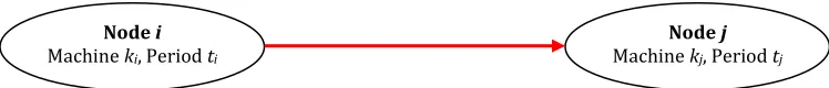
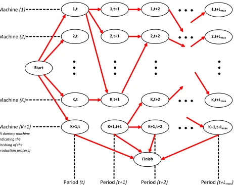
The network structure of the Column Generation subproblem is shown in Figure 2.2. The network consists of nodes that correspond to specific machines in specific time periods, and arcs that correspond to transfer of products from one machine to another while passing from one production stage to another. According to this structure, an arc exists from node ( to node only if there is a production path suggesting that the product should be processed at machine in period , and at machine in period . Other arcs in the network are artificial, and they have a zero arc weight, so that they wouldn’t have any effect in the selection of the longest path.
The arc costs for the longest path network should be determined so that the existing production paths have total arc weight ∑ ∑ ∑ ∑ , as this expression constitutes the objective value of the subproblem that needs to be maximized. For this purpose, the first and the third components are partitioned into machines; while the second and the fourth components are partitioned into time periods. When this logic is generalized, the arc costs between two nodes are determined as follows:
Figure 2.1: Representation of Two Nodes and an Arc in the Subproblem Network Node i
Machine ki, Period ti
{
∑
∑
∑
∑
where denotes the set of node pairs where a product can be processed at machine in period , and at machin in period .
Machine (1)
Machine (2)
Machine (K)
Machine (K+1)
(A dummy machine indicating the finishing of the production process)
Period (t) Period (t+1) Period (t+2) Period (t+Lmax)
Start
1,t+1
2,t+1
K,t+1
K+1,t+1 1,t
2,t
K,t
K+1,t
1,t+2
K,t+2
K+1,t+2 2,t+2
1,t+Lmax
K,t+Lmax
K+1,t+Lmax
2,t+Lmax
The Longest Path Problem for a graph with source node and sink node can be formulated as follows:
Indices:
denote the nodes in the network
denotes the arcs in the network
Parameters:
: Weight of arc , determined by the method explained above, so that the optimal solution of the subproblem corresponds to the column with maximum reduced cost in the master problem
Decision Variables:
{
∑
∑
∑
{
The master problem and subproblems of our Column Generation approach are built and solved using IBM Optimization Programming Language (OPL) (IBM, 2011). It is also noticeable that there are relatively efficient algorithms that solve the Longest Path Problem; but we solve it using linear programming, which is probably less efficient in terms of solution time.
D.
Direct Product Mix Formulation
machines. It does not use any allocation variables and its capacity constraints, which are defined for very specific sets of alternative machine types, only contain variables indicating the release quantities of each product type in each period.
Leachman and Carmon (1992) present a systematic Capacity Set Generation Procedure (CSGP) for generating alternative machine sets, and formulate capacity constraints for each of these generated sets. The design of such capacity constraints requires defining two sets: a set of machine types whose capacities are summed to form the right hand side of the constraint, and a set of operations (product-steps) whose capacity usages are summed to form the left-hand side of the constraint.
The CSGP is defined with the following three steps:
Step 1. List all alternative machine types capable of performing one or more operations (product-steps). The set of operations should include all operations that load the identified set of machine types or any proper subset.
Step 2. For all machine sets identified in Step 1 that have elements in common, form unions of these machine sets and unions of the corresponding operations. Here, larger sets are formed.
Step 3. Continue forming unions of intersecting machine sets so as to combine sets created in Step 2 with each other of with sets identified in Step 1. Terminate when no new machine sets can be generated.
The worst-case complexity of CSGP is shown to be , where is the maximal cardinality of the alternative machine sets, K the number of machine nodes of the maximal connected component of the bipartite graph of product-steps and machine types, and
N the number of product-steps in the problem data. Although the procedure is exponential, it is said to be practically useful since , the maximal number of machine types in a connected component of the bipartite graph, is typically relatively small, especially in semiconductor manufacturing settings.
Table 2.1: Data for CSGP Example
Operation Machines
A 1, 2
B 1, 3
C 1
D 2
E 1, 2, 3
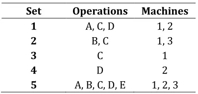
Table 2.2: Outcome of CSGP Example
Set Operations Machines
1 A, C, D 1, 2
2 B, C 1, 3
3 C 1
4 D 2
5 A, B, C, D, E 1, 2, 3
The CSGP works with the following logic for this example:
- Operation A can be performed by machines 1 and 2, operation C can be performed by machine 1, and operation D can be performed by machine 2. Since the machine sets {1,2}, {1}, and {2} have elements in common, we can form a union to get operation set {A, C, D} and machine set {1,2}.
- Operation B can be performed by machines 1 and 3. The machines that can perform operation C (namely machine 1) is a subset of machine set {1, 3}. Therefore we can form a union set containing operations {B, C} and machines {1, 3}.
- The set containing operation {C} and machine {1}, and the set containing operation {D} and machine {2} must also considered as sets by themselves (along with the union sets containing them).
- When we add the first two union sets, namely {A, C, D, 1, 2} and {B, C, 1, 3}, together; we must also add operation E, since it can be performed by all the machines in machine set {1, 2, 3}. Therefore, the set generated by the union of the union sets becomes {A, B, C, D, E, 1, 2, 3}.
All the sets generated by CSGP for this example are given in Table 2.2.
Let machine 1 with available capacity of 100 minutes perform operation A in 2 minutes, and operation B in 4 minutes; and machine 2 with available capacity of 900 minutes perform operation A in 6 minutes, and operation B in 12 minutes. If we set machine 1 to be the “standard machine”, then the corrected process times of machine 2 would be 2 minutes for operation A, and 4 minutes for operation B; and the corrected capacity of machine 2 would be
minutes. (Here, it must be noted that the uniformity assumption holds, since .) Since machine 1 is the standard machine, its process time and available capacity values are not corrected and they remain the same.
Once the alternative machine sets are generated and the aforementioned parameters are appropriately scales, the LP model presented below can be solved using the capacity constraints corresponding to the identified capacity sets.
Indices:
: Product type
: Time period
: Process step of product type , where and
Parameters:
: Average flow time of product from start to finish of its entire production process (“lead time” for the process)
: Average flow time for product from the start of its production process until initiation of step (“lead time” up to step )
: Estimated net discounted cash flow from producing and selling one unit of product in period
: Estimated cost of holding one unit of inventory of product at time
: Time required to process one unit of product in step (This parameter is corrected for different machine types, with regard to the “uniformity assumption”)
: The available capacity (in time units) of machine type in period (This parameter is also corrected with regard to the “uniformity assumption”)
: Production orders released to the system in period for product : Inventory of product at the end of period
∑( )
∑
∑
∑
∑
The number of variables appearing in capacity constraints each time period is equal to , the number of product types; so the total number of variables is , number of product types times number of time periods. The number of capacity constraints per period is the number of generated sets if machine types, which depends on the usage patterns appearing in the problem data. The cardinality of set can be as small as in the best case or as large as
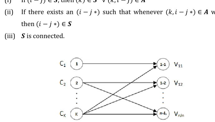
in the worst case. But Leachman and Carmon (1992) discuss that it is close the number of machine types for most practical cases, and the Direct Product Mix Formulation is usually only slightly larger than the standard production planning formulation that does not admit alternative machine types.
operations are satisfied, all capacity constraints for subsets of that machine set and its operation set are also satisfied. In order for a set to be considered a dominant cutset, it needs to satisfy the following three characteristics:
(i) If , then
(ii) If there exists an such that whenever we have , then
(iii) is connected.
Figure 2.3: Network Representation for Capacity Constraints of Direct Product Mix Formulation
Leachman and Carmon (1992) show that the dominant cutsets are the cutsets that correspond to the required capacity constraints in Direct Product Mix Formulation. They use Gale’s Flow Feasibility Theorem for Transshipment Networks (Gale, 1960) to show that cutsets for which one or more of the conditions above are violated are dominated by the cutsets that satisfy all the conditions above. Hence, the outcomes of CSGP (and equivalently, the dominant cutsets) generate the minimum number of capacity constraints that ensure capacity feasibility.
Even though the Direct Product Mix Formulation seems to be a good way of representing a multi-stage production system with alternative resources, it has a number of limitations that originate from the following assumptions:
(i) The set of machine types suitable for performing a particular processing step is independent of the machine types selected to perform other steps on the same product.
(ii) For each product there are exactly J process-steps (operations) loading one or more of the K machine types.
(iii) Production cost is independent of the product’s processing route.
assumption, within a particular machine set, the allocated machine hours of each machine type are scaled into “standard” machine hours according to a “standard” machine type.
The most limiting assumption of this formulation is the uniformity assumption, which may not always be satisfied in some production systems. The other three planning models presented in this chapter are not limited by this assumption; while the first two assumptions have to hold in all the formulations presented within the scope of this thesis. Path-Based model and the Column Generation approach require only assumptions (i) and (ii), while the Capacity Partition Approach also requires assumption (iii).
E.
Capacity Partition Approach
Hung and Cheng (2002) discuss two possible shortcomings of the Direct Product Mix Formulation, and suggested a solution approach to overcome them, called “Partition Approach”. The first and most important of these shortcomings is the uniformity assumption, and the second one is the union operation of two machine sets used in CSGP.
As mentioned earlier, uniformity assumption can cause serious inaccuracies in real life production planning problems. The method Hung and Cheng (2002) propose to relax the uniformity assumption is the Partition Approach, which divides the capacity of machines that can perform multiple jobs into partitions, and allocating each partition to a machine set in a manner similar to the Workload Allocation formulation of Leachman and Carmon (1992). This approach requires additional variables and constraints: Partition variables to represent each capacity portion for all machines, and equality constraints to enforce the sum of partition variables of a machine type to be equal to its capacity.
Hung and Cheng (2002) introduce the Capacity Partition Generation Procedure (CPGP) for their Partition Approach. CPGP is summarized below:
Step 1. List each operation and the machine set that performs it.
Step 3. Within each partition, perform a union on two machine sets with common machine types, and add the operations that can be performed by these machine sets.
Step 4. For each machine set in each partition, perform union operations until there is no more possible union within a partition.
Step 5. Designate a standard machine for each partition, and scale the available capacities and processing times according to the standard machine.
Step 6. Form the capacity constraint for each machines set of each partition and the capacity conservation constraint for each machine type.
CSGP, which is the set generation procedure that needs to be performed before solving the mathematical model in the Direct Product Mix Formulation, requires generating some machine sets initially and then forming unions of these machine sets to obtain new machine sets. As the number of machine sets increases, the number of capacity constraints increases, which can cause the size of the formulation to grow considerably. Hung and Cheng (2002) argue that the number of rows in an LP matrix usually affects solution time more than the number of columns, so a large number of capacity constraints can cause the Direct Product Mix Formulation to perform badly in terms of solution time. They show that the Partition Approach eliminates the union operation, and sometimes results in fewer capacity constraints. However, they conclude, after a series of experiments, that the LP models based on the union operation of CSGP do not require significantly more CPU time than the Partition Approach. Therefore, the Partition Approach ensures accuracy when uniformity assumption is not satisfied, but it does not provide an advantage in terms of solution time by eliminating the union operation.
An example for the CPGP is presented below.
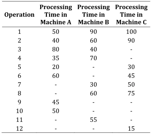
Table 2.3 shows the operation and processing time data for a production system with three machines: Machine A, Machine B, and Machine C. The distribution of operations on the machines is shown in Figure 2.4.
particular example, operation sets {5, 6}, {7, 8}, and {9, 10} can be performed on same machines; so the unions are formed. The resulting partitions can be observed in Table 2.4. The next step of the CPGP is building the capacity constraints corresponding to these partitions. In this example, there will be nine capacity constraints for each partition, and three constraints (one for each machine) to ensure that the sum of partition capacities equals available machine capacity.
Table 2.3: Data for CPGP Example
Operation Processing Time in Machine A
Processing Time in Machine B
Processing Time in Machine C
1 50 90 100
2 40 60 90
3 80 40 -
4 35 70 -
5 20 - 30
6 60 - 45
7 - 30 50
8 - 60 75
9 45 - -
10 50 - -
11 - 55 -
12 - - 15
Figure 2.4: Capacity Partitions for CPGP Example
Table 2.4: Outcome of CPGP Example
Partition Index Partition
1 {A, B, C, 1} 2 {A, B, C, 2}
3 {A, B, 3}
4 {A, B, 4}
5 {A, C, 5, 6} 6 {B, C, 7, 8}
7 {A, 9, 10}
8 {B, 11}
9 {C, 12}
1,2 7,8
9,10
11 12
A
The mathematical model based on the Partition Approach is as follows:
Indices:
: Product type
: Machine type
: Operation
: Partition
: Machine set contained in a partition
Parameters:
̂ : Processing time of operation on product by standard machine ̂ of partition
̂ : The factor used in converting original machine hours of machine to standard machine hours in partition
: Number of machine sets in partition : The nth machine set contained in partition
: The set of operations that can be performed by machine set of partition : The set of partitions that contain machine
: The flow time of product from the start of its production until operation : The flow time of product for its entire production route
: Available capacity (machine hours) of machine in time period
: The maximum cumulative quantity of product that can be sold by the end of period : The minimum cumulative quantity of product that can be sold by the end of period : The net profit from producing and selling one unit of product in time period : The backorder cost of product in time period
: The cost of holding one unit of product in time period
Decision Variables:
: Machine hours of machine type allocated to partition in period : The quantity of product that will be released in period
∑ ∑( )
∑ ̂
∑ ̂
∑
∑
∑
The number of production variables is the same as Direct Product Mix Formulation, which is , number of product types times number of time periods. However, there are also partition variables in this formulation, different than the previous one; and the number of partition variables is , where is the number of machine types, the number of partitions, and the number of time periods.
There is one capacity constraint for each machine set in each partition, so the number of capacity constraints is equal to the total number of machine sets. In addition to capacity constraints, there are also constraints that ensure that sum of partition capacities is equal to the available machine capacity. The number of such constraints is .
As mentioned earlier, the number of partition variables and capacity constraints depends on the machine usage pattern appearing in the problem data. As Hung and Cheng (2002) point out, there will be partitions in the best case; hence there will be a total of
Partition Approach will behave the same as Direct Product Mix Formulation; hence total number of constraints regarding capacity will be – .
3.
Design of Experiments
The purpose of our computational experimentation is to observe how our Column Generation formulation performs, and whether or not our claims about the approach were valid. Our hypothesis regarding the CG approach is that it would work efficiently in large problems, because the LP solution would assign nonzero production variables to a very small fraction of the possible process paths in a production environment with alternative process paths. This premise motivated us towards experimenting on different production environments to see what proportion of paths are being assigned nonzero production variables. We also wish to compare the computational performance of the CG approach to the performance of PB formulation, in terms of solution time. For this purpose, some time measures related to these two approaches are compared. These time measures will be discussed in detail in Chapter 4.
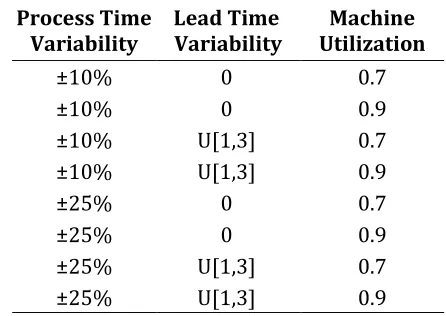
We hypothesized that the two main factors that would affect the performance of our Column Generation approach would be problem size, as expressed by the number of alternative production paths, and level of distinction between different paths. If some paths are markedly better than others in terms of cost and lead time, we would expect an optimal solution to use these paths predominantly. If, on the other hand, the cost differences between different paths tend to be very small, we would expect a great many slightly different paths to appear in an optimal solution. For observing the effects of these factors, the data sets are generated to examine the effect of different values of five key parameters: number of stages, number of machines at each stage, process time variability, lead time variability and machine utilization.
Number of Stages: This parameter denotes the number of process stages in the production system, which is one of the two determinants of problem size. It takes three values: 2, 4, and 6.
Number of Machines at Each Stage: This parameter denotes the number of alternative machines at each stage, which is the other factor determining the problem size. It takes three values: 2, 4, and 6.
Process Time Variability: This parameter is defined as the difference between process times of machines that perform the same operation. In other words, it determines how much the machines at a particular stage differ from each other. It takes two values: ±10%, and ±25%.
and , where denotes the process time variability and the mean processing time for that stage.
Lead Time Variability: This parameter shows whether or not lead time differs from one machine to another within a given stage. It takes two values: 0 or U[1,3]; which means either there is no lead time variability and all lead time values are set to 1, or there is lead time variability and the lead time values are randomly generated to be an integer between 1 and 3.
Machine Utilization: This parameter is defined as the target machine utilization, and it determines what proportion of the available machine capacity will be used on the average. It takes two values: 0.7, which demonstrates an average utilization level, and 0.9, which demonstrates a high utilization level.
The Column Generation approach is tested with 360 different problems, with 72 different settings and five replications in each setting. The different settings are generated by combining all possible values of the five parameters described above. As it can be seen on Table 3.1, there are nine possible problem sizes, and eight possible combinations of other production environment parameter levels.
Data sets are generated and managed using VBA in Microsoft Excel. Detailed information on data generation, including the parameter values that are the same for all production settings and how each mathematical model input is calculated, can be found in Appendix A.
Table 3.1: Design of Experiments with Different Values of Parameters
Number of Stages Number of Machines
at Each Stage Process Time Variability Lead Time Variability Utilization Machine
2 2 ±10% 0 0.7
2 4 ±10% 0 0.9
2 6 ±10% U[1,3] 0.7
4 2 ±10% U[1,3] 0.9
4 4 ±25% 0 0.7
4 6 ±25% 0 0.9
6 2 ±25% U[1,3] 0.7
6 4 ±25% U[1,3] 0.9
6 6
4.
Computational Results
A.
Proportion of Generated and Used Columns
While suggesting the solution approach and designing the experiments, we predicted that only a small proportion of possible columns would actually be generated by the Column Generation (CG) approach and assigned a non-zero production quantity, even though the number of all possible paths is very large. To verify this hypothesis, we consider the following two performance measures in our computational experiments:
Proportion of Generated Columns: This measure is given by the number of generated columns divided by the number of all possible columns, which is given by the number of possible production paths times the number of time periods. Recall that in a production system with stages and alternative machines at each stage, the total number of possible columns, i.e., the number of decision variables in the path-based model described in Chapter 2, is given by
.
Proportion of Used Columns: This measure is defined as the number of columns whose associated decision variable is positive, representing the number of paths actually used in production in some period, divided by the number of all possible columns.
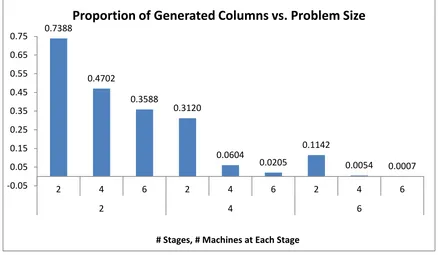
Figure 4.1: Proportion of Generated Columns with Changing Problem Size
0.7388
0.4702
0.3588
0.3120
0.0604
0.0205
0.1142
0.0054 0.0007
-0.05 0.05 0.15 0.25 0.35 0.45 0.55 0.65 0.75
2 4 6 2 4 6 2 4 6
2 4 6
# Stages, # Machines at Each Stage
Our results show that the Column Generation approach gets more and more efficient as problem size increases. Figure 4.1shows the proportion of generated columns as a function of the problem size, defined by the number of production stages and the number of machines in each stage. The proportion of generated columns decreases as problem size increases, and gets as small as 0.0007 on the average.
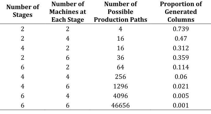
Table 4.1: Proportion of Generated Columns vs. Number of Possible Paths
Number of Stages Number of Machines at Each Stage Number of Possible Production Paths Proportion of Generated Columns
2 2 4 0.739
2 4 16 0.47
4 2 16 0.312
2 6 36 0.359
6 2 64 0.114
4 4 256 0.06
4 6 1296 0.021
6 4 4096 0.005
6 6 46656 0.001
Figure 4.2: Proportion of Generated Columns with Changing Number of Possible Paths
0 0.05 0.1 0.15 0.2 0.25 0.3 0.35 0.4
36 536 1036 1536 2036 2536
(# Ge n e rate d Co lu m n s) / (# A ll Possi b le Colum n s)
# Possible Paths
Table 4.1 shows the proportion of generated columns for different values of problem size, expressed as the number of possible production paths. Figure 4.2 shows how the proportion of generated columns changes with the number of possible paths. The proportion of generated columns decreases exponentially with increasing number of paths.
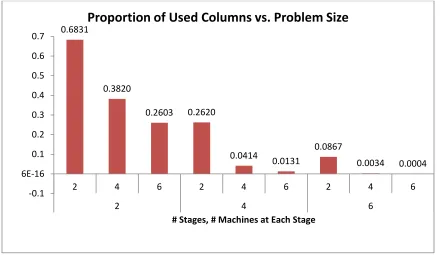
Figure 4.3: Proportion of Used Columns with Changing Problem Size
Table 4.2: Proportion of Used Columns vs. Number of Possible Paths
Number of Stages
Number of Machines at
Each Stage
Number of Possible Production Paths
Proportion of Used Columns
2 2 4 0.683
2 4 16 0.382
4 2 16 0.262
2 6 36 0.260
6 2 64 0.087
4 4 256 0.041
4 6 1296 0.013
6 4 4096 0.003
6 6 46656 0.0004
The proportion of used columns changes with changing problem size in a similar way to the proportion of generated columns. As seen in Figure 4.3, the proportion of used columns
0.6831
0.3820
0.2603 0.2620
0.0414 0.0131 0.0867
0.0034 0.0004
-0.1 6E-16 0.1 0.2 0.3 0.4 0.5 0.6 0.7
2 4 6 2 4 6 2 4 6
2 4 6
# Stages, # Machines at Each Stage
decreases with increasing problem size. Table 4.2 and Figure 4.4 suggest that the decrease in the proportion of used columns seems to be exponential.
Figure 4.4: Proportion of Used Columns with Changing Number of Possible Paths
B.
Solution Times of CG, and Comparison with PB
In this section we shall examine the computation times of the Path-Based and CG formulations. It is important to note that our CG implementation cannot be expected to compete with the Path-Based formulation in terms of solution time for several reasons. First of all, the CG method involves considerable overhead in terms of reading data files and constructing subproblem instances as well as the control logic for the CG approach that are not needed in the Path-Based model. Secondly, we have made no attempt to engineer our implementation of the CG method for efficiency. Several steps that could be taken in that direction include efficient implementation of the shortest path algorithm used to solve the subproblems, instead of solving as a linear program; restarting the master problem at each iteration from the final basis of the previous iteration, as opposed to restarting the solution of the master problem from scratch; and improving the efficiency of reading and outputting data through a more sophisticated OPL implementation. All these issues can be addressed directly if the CG method is implemented in a programming language like C++. However, our intention in this thesis is to explore the potential
0 0.1 0.2 0.3
36 536 1036 1536 2036 2536
(# Us
e
d
C
o
lu
m
n
s) /
(
# Al
l Possi
b
le
Co
lu
m
n
s)
# Possible Paths
Proportion of UsedColumns vs.
of the CG method for large problems with many alternative routings, by examining the number of columns actually generated and used.
We define the following performance measures:
Solve Time: The time, expressed in milliseconds, it takes to actually solve the mathematical models, both in the Column Generation approach and the Path-Based approach. This measure of time excludes all types of initialization, data reading, data modification, model building, or result interpretation processes. It only measures the time it takes for the LP solving algorithm to find the optimal solutions to the LP problems. For Column Generation (CG) approach, this time measure is the total time it takes to solve all the master problems and subproblems, since this approach iteratively solves these problems multiple times. For Path-Based (PB) approach, this time measure only denotes the time to solve the Path-Path-Based model once.
Data Time: The time, expressed in milliseconds, it takes to manage the data. This includes the time required to read initial data from Excel files, organize and modify the data into the format that the mathematical model requires, make necessary calculations to build the mathematical models, and transform the model outcomes into the necessary format. Most of these actions are required for CG approach, but still, data time is measured for PB approach as well.
Figure 4.5: Solution Time Outcomes for CG Approach
0 1000000 2000000 3000000 4000000 5000000 6000000 7000000 8000000 9000000
2 4 6 2 4 6 2 4 6
2 4 6
Ti m e ( m ill isec o n d s)
# Stages, # Machines at Each Stage
![2 Bromo 5 tert butyl N methyl N [2 (methylamino)phenyl] 3 (1 methyl 1H benzimidazol 2 yl)benzamide](data:image/gif;base64,R0lGODlhAQABAIAAAP///wAAACH5BAEAAAAALAAAAAABAAEAAAICRAEAOw==)