Generalized Sensitivity Analysis for Delay Differential Equations
H. T. Banks, Danielle Robbins and Karyn L. Sutton Center for Research in Scientific Computation Center for Quantitative Science in Biomedicine
North Carolina State University Raleigh, NC 27695-8212
March 8, 2012
Abstract
We present theoretical foundations for traditional sensitivity and generalized sensitivity func-tions for a general class of nonlinear delay differential equafunc-tions. Included are theoretical results for sensitivity with respect to the delays. A brief summary of previous results along with several illustrative computational examples are also given.
1
Introduction
Delay differential equations (DDEs) have been used for a number of years to model biological, phys-ical, and sociological processes, as well as other naturally occurring oscillatory systems. Minorsky [59] in 1942 was among the first to introduce the idea of hystero-differential equations, using these type of equations to explain self-excited oscillations arising in dynamic stabilization systems. He proposed [59, 60, 61] that some natural phenomena such as self-oscillations may be effected by the previous history of a motion or action as described by a retarded dynamical system. A retarded dynamical system is a system that describes an action that has delayed time dependence. The simplest of these physical systems are usually classified into systems with retarded damping given by
¨
x(t) +Kx˙(t−τ) +bx(t) =g(t), (1.1) or those with retarded restoring force described by
¨
x(t) +Kx˙(t) +bx(t−τ) =g(t), (1.2) wheregis some external force. Specifically, Minorsky used models such as (1.1) and (1.2) to study stabilization systems in ships. It is has been well understood for many years [30] that the infinite degree of the corresponding characteristic equation for a DDE such as (1.1) or (1.2) allows for an infinite number of eigenvalues for even a scalar DDE. This can promote dramatically different (from an ordinary differential equation) solution behavior such as self-excited oscillations in the solution [61]. This property of the DDE along with the widespread presence of delays in many physical and biological systems makes DDEs very important in modeling and control in these systems. Minorsky also provided insight as to the use of a nonlinear DDE to model a system with self-excited oscillations, as a linear DDE is unable to capture all of the properties of the self-excitation. Thus Minorsky lays a foundation for modeling oscillatory phenomena in general systems.
equation, to describe the dynamics of circular causal systems. A circular causal system is any causal system (one with current solution values depending only on current or past inputs) where changes to one part of the system effects another part of the system at a different rate so that the system does not go extinct. Parasite-host interaction is an example of an ecological circular causal system; if a parasite can complete its life cycle without killing the host or drastically altering the growth of the host population, the host population will continue to exist [50, 55]. The delay in this model can represent various naturally occurring phenomena such as the gestation period in a growing population, the life cycle of a parasite, cell cycle delays, etc. Hutchinson’s equation (to be used in the numerical illustrations below), its variations and other delay systems have also been used to model physiological control systems as well as numerous other biological processes [1, 23, 24, 26, 34, 35, 36, 37, 39, 40, 43, 44, 46, 47, 49, 53, 55, 56, 66]. This wide spread use of delay equations in applications has continued since the early contributions of Minorsky and Hutchinson. In the 1970’s and 80’s much work was done on foundations of delay systems, in contributions both theoretical and qualitative [30, 38, 39, 48] as well as computational (see [4, 5, 6, 7, 8, 9, 20, 52, 54] and the references therein) in nature. In some of these early efforts, parameter estimation and control system questions led to the investigation oftraditional sensitivity functions (TSFs)for delay systems. These TSFs and a more general concept ofgeneralized sensitivity functions (GSFs)
are the focus of our investigations in this paper. In one early paper [12], Banks, Burns and Cliff observed difficulty when estimating the delay and they suggested that this could be due to the fact that solutions of DDEs may not always be differentiable with respect to the delays; this makes estimation methods such as least squares and maximum likelihood challenging if derivative-based optimization routines are used. These authors also suggested the need for a formal theory regarding the existence of sensitivity functions with respect to the delay. Gibson and Clark [45] and Brewer [31] were among the first to treat theoretical questions of sensitivity for linear DDEs. In both contributions, these authors reformulated the delay system (as was done in the early semigroup approximation efforts of Banks, Burns and Kappel [8, 9, 20]) as an abstract system
˙
z(t) = A(q)z(t) +Bu(t), t≥0
z(0) = z0 = (η, ϕ), (1.3) where (η, ϕ) ∈Z ≡Rn×L2(−r,0;Rn),q ∈Q and the infinitesimal generatorA(q) is defined such that
A(q)(ϕ(0), ϕ) = (L(q)ϕ,ϕ˙). Then givent≥0,S(t;q) :Z →Z is defined such that
S(t;q)(η, ϕ) = (x(t;q), xt(q))
where S(t;q) is a strongly continuous semigroup and xt(ξ) = x(t+ξ), −r ≤ξ ≤ 0. By defining
As a result of the existence of the Frech`et derivatives, he is able to carefully and rigorously define sensitivity equations with respect to the parametersincluding the delay for the abstract system.
In a more recent report [2], Baker and Rihan formally derive sensitivity equations for delay differential equation models, as well as the equations for the sensitivity of parameter estimates with respect to observations (these latter sensitivities are what we shall discuss below as Generalized Sensitivity Functions (GSFs)). They consider a general nonlinear system of parameter dependent delay differential equations with parameterp∈RL given by
˙
x(t, p) = f(t, x(t), x(t−τ), p), t≥0, (1.4) x(t, p) = ψ(t, p), t≤0,
and investigate methods for sensitivity functions with respect to the parametersp and delayτ. Baker and Rihan offer an outline on how to numerically compute both TSFs and GSFs for retarded delay differential equations (as well as for neutral delay differential equations which are not discussed here in any generality). While their focus is on computational methods, they also list issues that arise when carrying out parameter estimation in DDEs. As we have already noted earlier, these include difficulty in establishing existence of the derivatives of the solution with respect to the parameters and the delays, as well as difficulty in establishing well-posedness for the derived sensitivity equations. Some of these issues are dealt with in a rigorous manner below.
Banks and Bortz [11] were among the first to consider sensitivity with respect to distributional delays. They used sensitivity analysis to show how changes in distributed parameters will effect the solutions of their nonlinear delay differential equation model for HIV progression at the cellular level where intracellular processing delays are distributed across cell populations. The models are validated with what is calledaggregate data [7].
When deriving the sensitivity equations Banks and Bortz obtain a system of DDEs, which are assumed to be well-posed. In their discussion of well-posedness for these sensitivity equations they assume the delay distributions are differentiable and parameterizable by a mean and standard deviation. In [11] they use theoretical steps (i.e., successive approximations, fixed point theory, Lipschitz continuity, etc.) employed in [10] to prove existence and uniqueness of the resulting sensitivities and sensitivity equations. Motivated by the efforts in [11], Banks and Nguyen [25] develop a rigorous theoretical framework for sensitivity functions for general nonlinear dynamical systems in a Banach space X where the parametersµ are themselves members of another Banach space M. In this setting they consider the sensitivity of solutionsx with respect to parameters µ in the following type of abstract nonlinear ordinary differential equations
˙
x(t) = f(t, x(t), µ), t≥t0 (1.5)
x(t0) = x0,
where f : R+×X × M → X and M and X are complex Banach spaces. They establish well-posedness for (1.5), and existence of Frech`et derivatives of the solution x(t) with respect to the parameters µ. As a result, there is a unique solution to the corresponding sensitivity equation
˙
y(t) = fx(t, x(t, t0, x0, µ), µ)y(t) +fµ(t, x(t, t0, x0, µ), µ), t≥t0 (1.6)
y(t0) = 0,
is developed for sensitivity theory using directional derivatives where the parameter space M is taken as the convex metric space of probability measures (including discrete, continuous or convex combinations thereof) taken with the Prohorov metric topology [7]. Below we give new results for sensitivity with respect to discrete delays. The proofs, given in [27], while quite tedious, continue with an adaption of the well known ideas for existence and uniqueness of the Frech`et derivative with respect to the delay in nonlinear DDE as employed in [11, 18, 25]. Very recent efforts, especially in areas of biology, demonstrate the continuing interest and importance of sensitivity equations in the sciences. For example Burns, Cliff, and Doughty [34] explain the use of continuous sensitivity equations for DDE models arising in a model for Chlamydia Trachomatis, while Kappel [53] discusses generalized sensitivities in dynamics of threshold-driven infections.
2
Solutions and their approximation
We first summarize some fundamental well-posedness and approximation results that have been recently developed elsewhere [7, 64]. We consider nonlinear nonautonomous dynamical systems involving delays of the general form
˙
x(t) =G(t, x(t), xt, x(t−τ1), . . . , x(t−τm), θ) +G2(t), 0≤t≤T, (2.1)
x(ξ) =ϕ(ξ), −r ≤ξ≤0,
where G=G(t, η, ψ, y1, . . . , ym, θ) : [0, T]×X×Rnm×Rp → Rn. Here X =Rn×L2(−r,0;Rn), 0 < τ1 < . . . < τm = r, xt denotes the usual function xt(ξ) = x(t+ξ), −r ≤ ξ ≤ 0, and
ϕ∈H1(−r,0).
The theoretical results in this manuscript will be illustrated computationally, and therefore, the solutions will need to be approximated. In order to approximate solutions, one may first convert them to an abstract evolution equation and then approximate in a space spanned by piecewise linear (or even higher order) splines (i.e., in a Galerkin approach, which is equivalent to a linear finite element approximation in partial differential equations). One is then able to numerically calculate the generalized Fourier coefficients of approximate solutions relative to the splines, and with these coefficients, recover an approximation to the solutions of (2.1).
We turn to the mathematical aspects of these nonlinear functional differential equations (FDE) systems and present an outline of the necessary mathematical and numerical foundations. First we describe the conversion of the nonlinear FDE system to an abstract evolution equation (AEE) as well as provide existence and uniqueness results for a solution to the FDE. One can use the ideas of the linear semigroup framework, in which approximation of linear delay systems has been developed, as a basis for a wide class of nonlinear delay system approximations. Details in this direction can be found in the early work [5, 6, 52] which is a direct extension of the results in [8, 9, 20] to nonlinear delay systems. We then provide a fundamental approximation framework including convergence results.
We shall make use of the following hypotheses throughout our presentation. (H1) The function Gsatisfies a global Lipschitz condition:
|G(t, η, ψ, y1, . . . , ym, θ)−G(t,η,˜ ψ, w˜ 1, . . . , wm, θ)|
≤K
(
|η−η˜|+|ψ−ψ˜|+
m
∑
i=1
|yi−wi|
)
for some fixed constantK and all (η, ψ, y1, . . . , ym), (˜η,ψ, w˜ 1, . . . , wm) inX×Rnm uniformly
(H2) The function G: [0, T]×X×Rnm×Rp→Rn is differentiable.
Remark 1. If we define the function g : [0, T]×Rn×C(−r,0;Rn)×Rp ⊂[0, T]×X×Rp → Rn given by
g(t, x, θ) =g(t, η, ψ, θ) =G(t, η, ψ, ψ(−τ1), . . . , ψ(−τm), θ), (2.2)
we observe that even though G satisfies (H1), g will not satisfy a continuity hypothesis on its domain in theX norm.
Letting z(t) = (x(t), xt)∈X, where the Hilbert space X has the inner product
⟨(η, ϕ),(ζ, ψ)⟩X =⟨η, ζ⟩Rn+
∫ 0
−r
⟨ϕ(ξ), ψ(ξ)⟩Rndξ, (2.3)
we define the nonlinear operatorA(t, θ) :D(A)⊂X→X by
D(A)≡ {(ψ(0), ψ)|ψ∈H1(−r,0)}
A(t, θ)(ψ(0), ψ) = (g(t, ψ(0), ψ, θ), Dψ) where here Dψ=ψ′. Then the FDE (2.1) can be formulated as
˙
z(t) = Az(t) +G2(t)
z(0) = z0, (2.4)
wherez0 = (x0, ϕ) is the initial condition andA=A(t, θ). For notational convenience we suppress the dependence on θin the remainder of this section.
Theorem 2. Assume that (H1) holds and let z(t;ϕ, G2) = (x(t;ϕ, G2), xt(ϕ, G2)), where x is the
solution of (2.1) corresponding to ϕ ∈ H1, G2 ∈ L2. Then for ζ = (ϕ(0), ϕ), z(t;ϕ, G2) is the
unique solution on [0, T]of
z(t) =ζ+ ∫ t
0
[A(σ)z(σ) + (G2(σ),0)]dσ. (2.5)
Furthermore, G2 → z(t;ϕ, G2) is weakly sequentially continuous from L2 (with weak topology) to
X (with strong topology).
These results can be established in one of several ways including fixed point theorem arguments or Picard iteration arguments. Either of these approaches can be used to establish existence, uniqueness and continuous dependence of the solution of (2.5). For existence, uniqueness and continuous dependence of the solution of (2.1), we note that our condition (H1) is a global version of the hypothesis of Kappel and Schappacher in [54], so that in the autonomous case their results also yield immediately the desired result for (2.1).
The uniqueness of solutions to (2.5) follows in the usual manner once we establish that A satisfies a dissipative inequality. Indeed, we define a weighting functionw on [−r,0) by
w(ξ) =j forξ ∈[−τm−j+1,−τm−j), j= 1,2, ..., m.
Then we consider solutions on the space Xw which is topologically equivalent to X, with the
weighted inner product
⟨(η, ϕ),(ζ, ψ)⟩w =⟨η, ζ⟩Rn+
∫ 0
−r
One can show without difficulty that (H1) implies the dissipative inequality (see [29, p. 71]) for the nonlinear operatorA(t)
⟨A(t)x− A(t)y, x−y⟩w ≤ω⟨x−y, x−y⟩w (2.7)
for all x, y∈ D(A) and all t.
The system of functional differential or delay equations described can now be simulated using an algorithm first developed by Banks and Kappel for linear systems [20] and extended in [5, 6]. Solutions are approximated in a space spanned by piecewise linear splines. Thus one can numerically calculate the generalized Fourier coefficients of the approximate solution in the spline basis representation and recover an approximation to the solution of (2.1).
Define XN to be an approximating subspace [20, 21] ofX. In particular, we chooseXN =X1N to be the piecewise linear spline subspaces of X discussed in detail in [20]. We briefly outline the results for the piecewise linear subspacesX1N (see Section 4 of [20]) given by
X1N ={(ϕ(0), ϕ)| ϕis a continuous first-order spline function with knots attNj =−jr/N, j= 0,1, . . . , N}.
A careful study of the arguments behind our presentation reveals that the approximation results given here hold for more general spline approximations. For example, if one were to treat cubic spline approximations (X3N of [20]), one would use the appropriate approximation analogues of Theorem 2.5 of [69] and Theorem 21 of [70] (e.g., see Theorem 4.5 of [69]). Hereafter when we write XN the reader should understand that we mean X1N of [20].
LetPN be the orthogonal projection in⟨·,·⟩wofX =XwontoXN. We define the approximating
operatorAN(t) =PNA(t)PN and consider the approximating equations in XN given by
zN(t) =PNζ+ ∫ t
0
[AN(σ)xN(σ) +PN(G2(σ),0)]dσ. (2.8)
These are equivalent to ˙
zN(t) =AN(t)zN(t) +PN(G2(t),0), zN(0) =PNζ, (2.9) the finite dimensional system inXN.
Define αN(t) so thatxN(t) = ˆβNαN(t) for any xN ∈XN. Here ˆ
βN = (βN(0), βN) whereβN = (eN0 , eN1 , . . . , eNN). The basis elements eN
j ’s are piecewise linear splines defined by the Kronecker symbol δij, so
eNj (ti) =δij fori, j= 0,1, . . . , N .
Then solving for zN(t) in the finite dimensional system (2.9) is equivalent to solving for αN(t) in the vector system
˙
αN(t) = ANαN(t) +PNG2(t)
αN(0) = αN0 , (2.10)
where ˆβNαN0 =PNz0 and AN is the matrix representation forAN. We note that having obtained
αN(t), the product ˆβNαN(t) converges uniformly intto the solutionz(t) = (x(t), xt) of (2.4) if we
can argue the convergencezN(t)→z(t). To do this for linear systems, one can use the Trotter-Kato
From (2.7) and the definition of AN in terms of the self-adjoint projections PN, we have at once that under (H1) the sequence {AN} satisfies onX a uniform dissipative inequality
⟨AN(t)x− AN(t)y, x−y⟩
w ≤ω⟨x−y, x−y⟩w (2.11)
for all x, y ∈ D(A) and all t. Uniqueness of solutions of (2.8) then follows immediately from this inequality. Upon recognition that (2.9) is equivalent to a nonlinear ordinary differential equation in Euclidean space with the right-hand side satisfying a global Lipschitz condition, one can easily argue existence of solutions for (2.9) and hence for (2.8) on any finite interval [0, T]. The next theorem, which ensures that solutions of (2.9) converge to those of (2.5), along with its proof is contained in [26].
Theorem 3. Assume (H1), (H2). Let ζ = (ϕ(0), ϕ), ϕ∈H1 and G2∈L2(0, T) be given, with zN
and z the corresponding solutions on [0, T] of (2.9) and (2.5), respectively. Then zN(t)→ z(t) = (x(t;ϕ, G2), xt(ϕ, G2)), asN → ∞, uniformly in ton [0, T].
Remark 4. One can actually obtain slightly stronger results than those given in Theorem 3. One can consider solutions of (2.5) and (2.9) corresponding to initial dataz0 = (x0, ϕ) =ζ withx0 ∈Rn,
ϕ∈L2 (i.e., ζ ∈X) and argue that the results of Theorem 3 hold also in this case.
The convergence given in Theorem 3 yields state approximation techniques for nonlinear FDE systems based on the spline methods developed in [20]. These results can be applied directly to control and identification problems, which are discussed in [5, 6].
3
Continuous dependence and differentiability
To establish continuous dependence in parameters and differentiability with respect to model pa-rameters, initial conditions, and discrete time delays (not previously done elsewhere for general nonlinear systems to the authors’ knowledge), we focus on a restricted case with nonlinear au-tonomous systems with one discrete delay of the form
dx(t)
dt =G(x(t), x(t−τ), θ), t >0 (3.1) x(ξ) =
{
ϕ(ξ), −τ ≤ξ <0 x0, ξ = 0
(3.2)
where x(t) ∈ Rn, x0 ∈ Rn, and θ ∈ Rp. While we consider here the case of finite dimensional model parameters the results also hold in a more general case when parameters are distributed, and hence infinite dimensional, as presented in [17, 18]. Once established, these results allow us to study the traditional and generalized sensitivity functions, where sensitivity is considered with respect to these three quantities. We begin by considering continuous dependence of solutionsx(t) on model parameters θ. We note that we focus on these quantities as they are often unknown in practice and may need to be estimated from observed or experimental data. The use of sensitivity functions can aid in that endeavor.
Lemma 5. Let G:Rn×Rn×Rp →Rn and for θ=θ0, letx(t, x0, ϕ, τ, θ0) be a solution of (3.1)
-(3.2)for t∈[0, T]. Assume that
lim
θ→θ0
uniformly in x and x˜. For (x1,x˜1, θ),(x2,x˜2, θ)∈Rn×Rn×Rp assume that
|G(x1,x˜1, θ)−G(x2,x˜2, θ)| ≤C1|x1−x2|+C2|x˜1−x˜2| (3.4)
where Cj > 0 is a constant for j = 1,2. Then the initial value problem (3.1)-(3.2) has a unique
solution x(t, x0, ϕ, τ, θ) that satisfies lim
θ→θ0
x(t, x0, ϕ, τ, θ) =x(t, x0, ϕ, τ, θ0), t∈[0, T].
Next, we turn to differentiability of the general system (3.1)-(3.2) with respect to model pa-rameters in the following theorem. The proof is excluded but can be found in [27, 64]. Also, the proof of Theorem 8 can easily be followed to give that of Theorem 6. Without further discussion, we then state Theorem 7, in which we establish differentiability of the model system with respect to the initial conditions, which is also proven in [27].
Theorem 6. Suppose thatG(x,x, θ˜ )has continuous Frech`et derivativesGθ, Gx, Gx˜such that|Gx| ≤
M0,|Gx˜| ≤M1, and|Gθ| ≤M2. Then the Frech`et derivativey1(t) = ∂x∂θ(t) ∈Rn×p exists and is the
unique solution for
˙
y1(t) =Gx(x(t), x(t−τ), θ)y1(t) +Gx˜(x(t), x(t−τ), θ)y1(t−τ) +Gθ(x(t), x(t−τ), θ),
y1(t) =0, −τ ≤t <0
Theorem 7. Suppose the functionG(x,x, θ˜ )of (3.1)has continuous Frech`et derivativesGx(x,x, θ˜ ),
Gx˜(x,x, θ˜ ), with respect to x and x˜, with |Gx| ≤ M0, |Gx˜| ≤ M1. Then the Frech`et derivative
y2(t) = ∂z∂0x(t, z0, θ) exists withy2(t)∈ L(Z,Rn) (recallz0 = (x0, ϕ), Z =Rn×L2(−τ,0;Rn)), and
satisfies the equation
˙
y2(t)[h] =Gx(x(t), x(t−τ), θ)y2(t)[h] +G˜x(x(t), x(t−τ), θ)y2(t−τ)[h], t >0 (3.5)
y2(ξ) =I −τ ≤ξ≤0,
where I ∈ L(Z,Rn) is the identity.
Finally we state results for derivatives with respect to the discrete delays with proofs being given in [27].
Theorem 8. Suppose that G(x,x, θ˜ ) has continuous Frech`et derivatives Gx, Gx˜ such that |Gx| ≤
M0, and |Gx˜| ≤M1 and suppose that the solution x of (3.1)-(3.2)satisfies
x∈H1,∞(−τ, T;Rn), for0< τ < r for fixedr >0. Then the Frech`et derivativey3(t) = ∂x∂τ(t) ∈Rn
exists and is the unique solution for
˙
y3(t) =Gx(x(t), x(t−τ), θ)y3(t) +Gx˜(x(t), x(t−τ), θ)[y3(t−τ)−x˙(t−τ)] (3.6)
y3(ξ) = 0, −τ ≤ξ≤0. (3.7)
4
Sensitivity functions
Given the above results, especially differentiability in the quantitiesθ, z0 = (x0, ϕ) andτ, we are now able to use the powerful sensitivity analytic techniques in delay systems. For further simplification in the remainder of our discussions we restrict our considerations to constant function initial conditions so in z0 = (x0, ϕ) we assume ϕ(ξ) = x0, −r ≤ ξ ≤ 0. Traditionally, sensitivity analysis is the quantification of the effect changes in parameters have on model solutions. Traditional sensitivity functions (TSFs), which are given by,
y1k(t) = ∂x
∂θk k= 1, ..., p
y2m(t) = ∂x
∂xl0 l= 1, ..., n y3(t) =
∂x
∂τ, (4.1)
are local in nature as they are defined by locally evaluated partial derivatives, i.e., ∂x∂θ(t,θ,¯ x¯0,τ¯), which gives information over specified time intervals, and at values of parameters, initial conditions and delays. Even with this limitation, these functions have been used to improve sampling in an experimental setting; specifically they can be used to guide the time at which measurements should be taken to best inform the estimation of unknown parameters [15, 16]. That is, sampling might be advisable in time intervals where, for example,yk1(t) is large, as it indicates that the model solution x(t) is sensitive to changes in the parameterθk. Similarly, insensitivity to a certain parameter (or
unknown quantity), indicated by small or zero values of the TSF, imply that observations can not be profitably taken in that region if the goal is estimation of the parameter.
TSFs may be approximated by forward differences, but are typically found by solving the system of sensitivity equations
d dt
∂x(t)
∂θ =
∂G ∂x
∂x ∂θ(t) +
∂G ∂x˜
∂x
∂θ(t−τ) + ∂G
∂θ(t) (4.2) for the corresponding system
dx(t)
dt = G(x(t), x(t−τ), θ), t >0
x(ξ) = x0, −r≤ξ≤0, (4.3) where the ∂θ∂ and dtd operators have been interchanged, due to the continuity assumptions made on G and x. We note that sensitivity analysis is most efficiently carried out in two steps. Once a solution x(t) corresponding to (¯θ,x¯0,τ¯) of the above (original delay) equation (4.3) is obtained, one uses this solution to evaluate the coefficients in system (4.2). This decoupling of the original equation and the sensitivity equation has implications when considering the sensitivity with respect to the time delay τ in one of the examples discussed below, which if solved in a coupled manner would result in a so-called neutral delay system.
inverse problem framework, not only to put our discussion in context, but also to define quantities in the definition of the GSFs.
Given a model solution x(t), the sensitivity of the solution to an estimated quantityqk (where
q= (θ, x0, τ)T) is
sk(t, q) =
∂f ∂qk
(t, q)∈Rm,
wheref(t, q) =h(t, x(t), x(t−τ), θ) are the model quantities corresponding to the observed data. Observations are typically available at discrete times, which we denote by t1, ..., tnd. The model
representation of the data is then
f(tj, q) =h(tj, x(tj), x(tj−τ), θ), j= 1, . . . , nd.
In general, the data are not exactly f(tj, q), due to uncertainty in the measurement process, and
also due to small fluctuations not explicitly included in the model. Therefore we represent the observation processYj at time tj by the statistical model
Yj =f(tj, q0) +Ej, j= 1, . . . , nd, (4.4)
where f(tj, q) = h(tj, x(tj), x(tj −τ), θ), q = (θ, x0, τ), for q ∈ Q = Rp ×Rn × R1. Here
q0 = (θ0, x00, τ0)T represents the ‘true values’ of the parameters that generates the observations
{Yj}nj=1d . The existence of q0 is commonly assumed [13], implying that (3.1) describes the biologi-cal, sociologibiologi-cal, or physical process essentially precisely.
The observation errors Ej are random variables, each with unknown but assumed independent
and identical probability distributions of mean zero, and constant variance σ2. Each data set
{yj}nj=1d is one realization of the random variable {Yj}nj=1d , and the corresponding errors are also a
realization of theEj. Estimating unknown quantities via the minimization between the model and
data assuming the statistical model (4.4) gives rise to the commonly used ordinary least squares (OLS) estimator
qOLS = arg min q∈Q
nd
∑
j=1
|Yj−f(tj, q)|2, (4.5)
where the objective functional is minimized over an admissible parameter spaceQ. Another com-mon formulation is a weighted least squares procedure, in which the error is assumed to be pro-portional to the model quantityf(tj;q), i.e., relative error. For a more complete discussion of the
underlying assumptions and related formulations, see [13].
The varianceσ2of the observation error is used in the computation of standard errors, confidence intervals, etc. and also in the generalized sensitivity functions. For a given set of data,{yj}nj=1d and parameter estimates ˆq, the (bias-adjusted) variance is estimated as
ˆ
σ2 = 1 n−np
nd
∑
j=1
|yj−f(tj,qˆ)|2 (4.6)
fornp=p+n+ 1 estimated parameters, where np =dim(Q).
The generalized sensitivity functions [16, 19, 72] are defined by
gs(t) =
∫ t
0 [
F(T)−1 1
σ2(s)∇qf(s, q 0)
]
for varianceσ2(t) that may possibly be time-dependent, true parametersq0, some general measure P that embodies the observations, and the Fisher information matrix (FIM)F which is defined by
F(T) = ∫ T
0 1
σ(t)∇qf(t, q 0)∇
qf(t, q0)TdP(t). (4.8)
We note that the definition of the measure P affects the FIM, and it can be chosen in such a way as to optimize the information from data concerning the estimated parameters. The GSFs are cumulative functions, such that at time tj, only the contributions of measurements up to and
including those at timetj are relevant. By the definition in (4.7), it is readily seen that the GSFs are
one at the final time gs(tnd) = 1. As discussed in [16, 72], regions over which the sharpest change
(either increase or decrease) of the GSFs indicate regions of high information content. Decreases in the GSF corresponding to a given parameter indicate correlation between that parameter and at least one other estimated parameter. In this case, it can be seen [16] that computing the GSF for one of the correlated parameters and holding the other(s) fixed, will result in a monotonically increasing GSF. Therefore, regions over which the GSF decreases indicate that the data in that region indeed contains information concerning that parameter, but it is correlated with at least one other parameter, and simultaneous identifiability of all parameters may be difficult.
As observations are typically available at discrete time points and our discussions are in the context of parameter estimation from observed or measured data, we have included here also the definitions for the GSFs and FIM for a discrete measure P =∑nd
j=1∆tj. In the discrete case, the
generalized sensitivity functions are
gs(tj) =
j
∑
i=1 1 σ2(t
j)
[
F−1× ∇qf(ti, q0)
]
· ∇qf(ti, q0), (4.9)
for observation times tj wherej= 1, ..., nd. In the above definition, the discrete FIM is given by
F =
nd
∑
j=1 1 σ2(t
j)∇
qf(tj, q0)∇qf(tj, q0)T, (4.10)
which measures the information content of the data corresponding to the parameters. In both (4.7) and (4.9), the estimate for the variance of the observation error is used up to and including the timetj of the observation, given by
σ2(tj) = j
∑
i=1
|yi−f(ti,qˆ)|2. (4.11)
If the variance is assumed constant (σ2(t) ≡ σ2), one would simply calculate the estimate as in (4.6), and use that in (4.7) or (4.9).
5
Illustrative computations
saturation is possible, but the death rate is proportional to previous population levels. The stan-dard logistic example (without delay) has been effectively used to illustrate with simulated data the ideas of traditional and sensitivity functions and how these techniques may improve data sampling for the purpose of parameter estimation [15, 16]. Therefore, it is natural to turn to the delayed logistic equation now that we are able to study sensitivity functions in systems involving a discrete delay. Here we will also numerically generate simulated data with a known delay, and demonstrate that the estimation can be improved using insights gained from the sensitivity function solutions.
The second example we use is also an ubiquitous model, the delayed harmonic oscillator of Minorsky discussed in the Introduction. As noted there, this example arises in many physical applications where oscillatory phenomena are important.
5.1 Hutchinson equation example
In his seminal paper [50] and book [51], Hutchinson arrived at a version of the logistic equation that incorporated a delay in the carrying or death rate term,
dx(t)
dt =rx(t) (
1−x(t−τ) K
)
. (5.1)
The model was suggested as a possible explanation of the growth dynamics seen in Daphnia. This population seemed to grow exponentially at low population sizes, but it would oscillate at higher population levels. Hutchinson hypothesized that this growth was like that of the logistic model, only that the population seemed to be able to exceed its carrying capacity and perhaps it was this value that the population level was oscillating around.
The traditional sensitivity functions with respect to the model parametersr, K, initial condition x0, and delay τ are given by
∂ ∂r
dx(t) dt =r
[
1−x(t−τ) K
] ∂x(t)
∂r −
rx(t) K
∂x(t−τ) ∂r +x(t)
[
1−x(t−τ) K
]
∂ ∂K
dx(t) dt =r
[
1−x(t−τ) K
] ∂x(t)
∂K −
rx(t) K
∂x(t−τ)
∂K +rx(t) [
x(t−τ) K2
]
∂ ∂x0
dx(t) dt =r
[
1−x(t−τ) K
] ∂x(t)
∂x0 −
rx(t) K
∂x(t−τ) ∂x0
∂ ∂τ
dx(t) dt =r
[
1−x(t−τ) K
] ∂x(t)
∂τ −
rx(t) K
[
∂x(t−τ)
∂τ −x˙(t−τ) ]
.
By changing the order of integration, and letting s1(t) = ∂x∂r(t), s2(t) = ∂x∂K(t), s3(t) = ∂x∂x(0t), and
s4(t) = ∂x∂τ(t), we have the system
∂s1(t)
∂t =r [
1− x(t−τ) K
]
s1(t)−
rx(t)
K s1(t−τ) +x(t) [
1−x(t−τ) K
]
(5.2) ∂s2(t)
∂t =r [
1− x(t−τ) K
]
s2(t)−
rx(t)
K s2(t−τ) +rx(t) [
x(t−τ) K2
]
(5.3) ∂s3(t)
∂t =r [
1− x(t−τ) K
]
s3(t)−
rx(t)
K s3(t−τ) (5.4) ∂s4(t)
∂t =r [
1− x(t−τ) K
]
s4(t)−
rx(t)
0 10 20 30 40 50 0
5 10 15 20
t
x (t)
(a) solutionx(t)
0 10 20 30 40 50
−20 0 20 40 60
t
ts (t)
r K x 0
(b) traditional sensitivity functionts(t)
0 10 20 30 40 50
−2 −1 0 1 2 3
t
gs (t)
r K x 0
(c) generalized sensitivity functiongs(t)
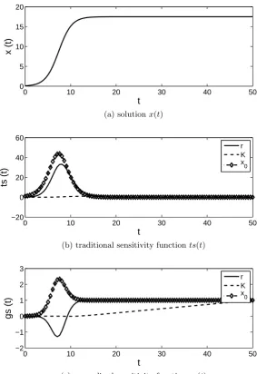
Figure 1: The numerical approximation to the solutions (a) for the Hutchinson equation, and the corresponding traditional (b) and generalized (c) sensitivity functions with respect to the model parameters r and K, and the constant initial value x0 are provided here for the values ¯r = 0.7,
¯
K = 17.5, and ¯x0 = 0.1.The generalized sensitivity functions were computed with constant variance
σ2= 0.1.
As noted earlier, we consider only the case of constant initial data, and thus we do not discuss here the Frech`et derivative y2(t) = ∂z∂0x(t, z0, θ) where z0 = (x0, ϕ), Z =Rn×L2(τ,0;Rn); the results of Theorem 7 still ensure the existence and uniqueness of the solution ∂x∂x(t)
0 10 20 30 40 50 0
5 10 15 20
t
x (t)
(a) solutionx(t)
0 10 20 30 40 50
−20 0 20 40 60 80
t
ts (t)
r K x 0 τ
(b) traditional sensitivity functionsts(t)
0 10 20 30 40 50
−2 −1 0 1 2 3
t
gs (t)
r K x 0 τ
(c) generalized sensitivity functionsgs(t)
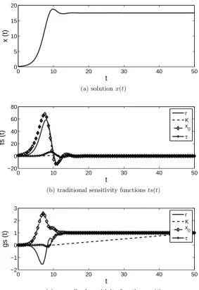
Figure 2: The numerical approximation for the solutions (a) to the Hutchinson equation with delay τ = 1, and corresponding traditional (b) and generalized (c) sensitivity functions with respect to growth rate r, carrying capacity K, constant initial state x0, and delay τ, each evaluated at (¯r,K,¯ x¯0,τ¯) = (.7,17.5, .1,1). The generalized sensitivity functions were computed with constant varianceσ2 = 0.1.
not unknown quantities but rather an input in the traditional sensitivity functions above.
0 10 20 30 40 50 0
10 20 30 40
t
x (t)
(a) solutionx(t)
0 10 20 30 40 50
−200 −100 0 100 200
t
ts (t)
r K x 0 τ
(b) traditional sensitivity functionsts(t)
0 10 20 30 40 50
−0.5 0 0.5 1 1.5
t
gs (t)
r K x 0 τ
(c) generalized sensitivity functionsgs(t)
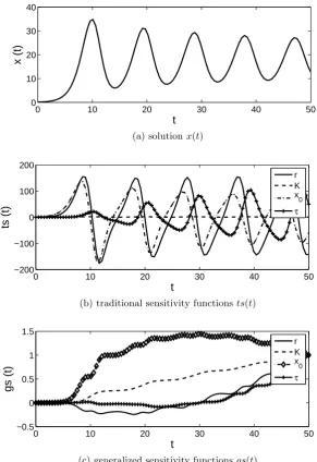
Figure 3: The numerical approximation for the solutions (a) to the Hutchinson equation with delay τ = 2πr ≈2.244, and corresponding traditional (b) and generalized (c) sensitivity functions with respect to growth rate r, carrying capacity K, constant initial state x0, and delay τ each evaluated at (¯r,K,¯ x¯0,¯τ) = (.7,17.5, .1,2¯πr). The generalized sensitivity functions were computed with constant varianceσ2 = 0.1.
initial conditionx0 and the growth rater simultaneously from data corresponding to this interval is likely problematic. As one would expect the solution appears to be sensitive to the carrying capacity essentially once it is approached. It is easier to see this in panel 1(c) than in 1(b), as the magnitude of the sensitivity to the other parameters (r and x0) is significantly greater. The definition of the generalized sensitivity functions is such that their magnitude is not as varied even with respect to different quantities.
Table 1: Estimation of delay τ
ˆ
τ RSS
tunif 0.9561 16.204
tGSF 1.032 6.575
carrying capacity but the effect is not sufficient for the oscillations to continue, and the solution approaches its carrying capacity x(t) → K around t = 14. It is around the time of the solution first exceeding and then decreasing to less than the carrying capacity (approximately, the interval t∈[8,11]), which can be interpreted as the effect of the delay, that the sensitivity function solutions can be interpreted to mean that the model solutionx(t) is sensitive to this delayτ. The solutions of the traditional and generalized sensitivity functions with respect to x0 and r together suggest that the beginning time interval of the solution is most sensitive to these quantities but that they are strongly correlated.
With a larger delay,τ = 2πr ≈2.244, the results given in Figure 3 reveal that many more oscilla-tions in the solutionx(t) occur, although they do dampen slightly. The traditional and generalized sensitivity functions for the unknown quantities q = (r, K, x0, τ) then indicate which parts of the oscillatory solution are most sensitive to the respective parameter qi. Regions of decreasing GSF
indicate correlation among parameters, as with the growth rater and initial conditionx0in Figures 1 and 2.
To illustrate the information gained from the solutions of the TSF and GSF with respect to the delay with a moderate delayτ = 1, we generated simulated data with 10% error and used this to estimate the delay τ, while holding the other parameters fixed. As seen in [16], any parameter correlation issues would be irrelevant and estimates should be improved if data is concentrated in any regions of enhanced information content (regions of greatest change in GSF or TSF).
0 2 4 6 8 10 12 14 16 18 20
−5 0 5 10 15 20
x(t,τ) data yj
(a) model solution: with ˆτ usingtunif
0 2 4 6 8 10 12 14 16 18 20
−5 0 5 10 15 20
x(t,τ) data yj
(b) model solution: with ˆτ usingtGSF
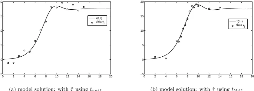
Figure 4: The solutions to the delay logistic equation with estimated delay ˆτ from data as shown in each graph: (a) ˆτ with data corresponding to tunif, (b) ˆτ with data corresponding to tGSF.
the delay is evident in that the estimated value for ˆτ = 1.032 is closer to the true valueτ0 = 1 than that ˆτ = 0.9561 when uniform data is used. Additionally the resulting residual sum of squares
RSS=
1 ∑
j=1
5|yj−f(tj,τˆ)|2
is less (i.e., a better fit to data) in the estimation with data concentrated in [8,11]. Model solutions corresponding to the estimated ˆτ’s overlayed with the data are shown in Figure 4(a) for simulated uniform data and with data concentrated in [8,11] in Figure 4(b).
5.2 Harmonic Oscillator
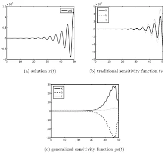
We turn finally to illustrating the use of the TSF and GSF for the Minorsky harmonic oscillators with delays as given in the Introduction. We recall that the equation with delayed damping has the form
d2x(t) dt2 +K
dx(t−τ)
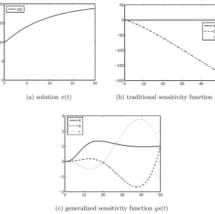
dt +bx(t) =g(t), (5.6) while the system with delayed restoring force is given by
d2x(t) dt2 +K
dx
dt +bx(t−τ) =g(t). (5.7) We use traditional and generalized sensitivity functions with equations (5.6) and (5.7) and illustrate their application in determining regions of sensitivity for model parametersK, band time delay τ. As before, we take the derivative of equation (5.6) with respect to each parameter qi,
whereq = (K, b, τ)T to obtain the TSF corresponding to that parameterqi. First, lettingx=x1(t) and x2(t) = ˙x(t), and rewriting equation (5.6) as a first order system we have
dx1(t)
dt =x2(t) dx2(t)
dt =g(t) =bx1(t)−Kx2(t−τ). (5.8) The traditional sensitivity functions are then solutions of
ds1(t)
dt =s4(t) ds2(t)
dt =s5(t) ds3(t)
dt =s6(t) ds4(t)
dt =−bs1(t)−Ks4(t−τ)−x2(t−τ) ds5(t)
dt =−bs2(t)−Ks5(t−τ)−x1(t) ds6(t)
dt =−bs3(t)−Ks6(t−τ) +Kx˙2(t−τ),
0 10 20 30 40 50 −1
−0.5 0 0.5 1 1.5x 10
5
y(t)
(a) solutionx(t)
0 10 20 30 40 50
−8 −6 −4 −2 0 2 4 6x 10
6
K b
τ
(b) traditional sensitivity functionts(t)
0 10 20 30 40 50
−30 −20 −10 0 10 20 30
K b
τ
(c) generalized sensitivity functiongs(t)
Figure 5: Depicted above are (a) the solution to the harmonic oscillator with delayed damping K =.5, b= 2,τ = 1, andg(t) = 10, (b) the traditional sensitivity functions and (c) the generalized sensitivity functions with respect to K, b, τ.
generalized sensitivity functions with respect to q = (K, b, τ)T. The solutions of the TSFs imply that the solution is sensitive to all three parameters, with the sensitivities varying in phase with each other, and beginning when the solution itself begins oscillating. This would suggest that there may be some correlation between these three parameters, since their regions of sensitivity are identical. The solutions to the generalized sensitivity functions, however, clarify this point, and indicate that it is the parameters K and b that are correlated and the delayτ is uncorrelated with the other two over its regions of sensitivity. Therefore, if one were to estimate parameters with this model, one should not expect to estimate both K and b simultaneously, but estimating either K or b does not affect one’s ability to estimate the delay τ. The solution is not sensitive to any of the parameters until the oscillations grow, indicating that data taken in the beginning time intervals should not be expected to contain much information about any of the parameters. It is not immediately obvious that two parameters K and τ appearing in the same term would be uncorrelated and therefore, both potentially are identifiable from data.
0 5 10 15 20 0
5 10 15 20
x(t)
(a) solutionx(t)
0 10 20 30 40 50
−200 −150 −100 −50 0 50
K b
τ
(b) traditional sensitivity functionts(t)
0 10 20 30 40 50
−2 −1 0 1 2 3
K b
τ
(c) generalized sensitivity functiongs(t)
is disproportionately sensitive to the restoring coefficient b as compared with K and τ. However, the generalized sensitivity functions provide additional insight in that the solution appears to be sensitive toK early on and while there are regions of increased information content relative to the delay τ, that the parameterb is, not surprisingly, correlated withτ, and one should not expect to identify both simultaneously with data sampled from those intermediate and later regions.
Concluding Remarks
After giving a brief survey of previous contributions on theoretical and computational aspects of traditional sensitivity functions for delay differential equation systems, we presented a summary of new theoretical results (proofs for which are given in [27]) for differentiation of solutions with respect to parameters, initial data and delays in general nonlinear delay differential equations. These results provide a theoretical foundation for the rigorous formulation of both traditional and generalized sensitivities for delay systems. We illustrate the ideas in the context of Hutchinson’s delayed logistic equation and the classical Minorsky harmonic oscillators with delayed damping or delayed restoring forces.
Acknowledgements
This research was supported in part by Grant Number NIAID R01AI071915-09 from the National Institute of Allergy and Infectious Disease, in part by the U.S. Air Force Office of Scientific Research under grant number FA9550-09-1-0226 and in part by the National Institute on Alcohol Abuse and Alcoholism under a subcontract from the Research Foundation for Mental Hygiene.
References
[1] J. Arino, L. Wang and G. Wolkowicz, An alternative formulation for a delayed logistic equation,
J. Theo. Bio.,241 (2006), 109–118.
[2] C. Baker and F. Rihan, Sensitivity analysis of parameters in modelling with delay-differential equations,MCCM Tec. Rep.,349(1999), Manchester, ISSN 1360-1725.
[3] H.T. Banks, Modeling and Control in the Biomedical Sciences, Lecture Notes in Biomath., Vol. 6, Springer-Verlag, Berlin, Heidelberg, New York, 1975.
[4] H.T. Banks, Delay systems in biological models: approximation techniques,Nonlinear Systems and Applications(V. Lakshmikantham, ed.), Academic Press, New York, 1977, 21–38.
[5] H. T. Banks, Approximation of nonlinear functional differential equation control systems, J. Optimiz. Theory Appl.,29 (1979), 383–408.
[6] H. T. Banks, Identification of nonlinear delay systems using spline methods, in: V. Lak-shmikantham (Ed.), Nonlinear Phenomena in Mathematical Sciences, Academic Press, New York, NY, 1982, 47–55.
[8] H.T. Banks and J.A. Burns, An abstract framework for approximate solutions to optimal control problems governed by hereditary systems, International Conference on Differential Equations(H. Antosiewicz, Ed.), Academic Press (1975), 10–25.
[9] H.T. Banks and J.A. Burns, Hereditary control problems: numerical methods based on aver-aging approximations,SIAM J. Control & Opt.,16(1978), 169–208.
[10] H.T. Banks, Identification of nonlinear delay systems using spline methods. InNonlinear Phe-nomena in Mathematical Sciences,V. Lakshmikanitham, Ed. Academic Press, Inc., New York, NY, 1982, pp. 47-45.
[11] H.T. Banks and D. M. Bortz, A parameter sensitivity methodology in the context of HIV delay equation models,Journal of Mathematical Biology,50(6) (2005), 607-625.
[12] H.T. Banks, J.A. Burns and E.M. Cliff, Parameter estimation and identification for systems with delays,SIAM J. Control and Optimization,19(1981), 791–828.
[13] H.T. Banks, M. Davidian, J.R. Samuels, Jr. and Karyn L. Sutton, An inverse problem sta-tistical methodology summary, CRSC-TR08-01, January, 2008; Chapter 11 in Mathematical and Statistical Estimation Approaches in Epidemiology, (edited by Gerardo Chowell, et al.), Springer, Berlin Heidelberg New York, 2009, pp. 249–302.
[14] H.T. Banks, J.E. Banks and S.L. Joyner, Estimation in time-delay modeling of insecticide-induced mortality, CRSC-TR08-15, October, 2008; J. Inverse and Ill-posed Problems, 17 (2009), 101–125.
[15] H. T. Banks, S. Dediu and S. L. Ernstberger, Sensitivity functions and their uses in inverse problems, CRSC-TR07-12, July, 2007; Journal of Inverse and Ill-Posed Problems,15 (2007), 683–708.
[16] H.T. Banks, S. Dediu, S. Ernstberger and F. Kappel, Generalized sensitivities and optimal ex-perimental design, CRSC-TR08-12 (Revised), November, 2009;J. Inverse and Ill-posed Prob-lems,18 (2010), 25–83.
[17] H.T. Banks, S. Dediu and H.K.Nguyen, Time delay systems with distribution dependent dy-namics, CRSC-TR06-15, May, 2006;IFAC Annual Reviews in Control,31(2007), 17–26. [18] H.T. Banks, S. Dediu and H. K. Nguyen, Sensitivity of dynamical systems to parameters in a
convex susbset of a topological vector space, CRSC-TR06-25, November, 2006;Mathematical Biosciences and Engineering,4 (2007), 403–430.
[19] H.T. Banks, K. Holm and F. Kappel, Comparison of optimal design methods in inverse prob-lems, CRSC-TR10-11, July, 2010;Inverse Problems,27(2011) 075002(31pp).
[20] H. T. Banks and F. Kappel, Spline approximations for functional differential equations, J. Differential Equations,34(1979), 496–522.
[21] H.T. Banks and K. Kunisch, Estimation Techniques for Distributed Parameter Systems, Birkhausen, Bosten, 1989.
[23] H.T. Banks and J.M. Mahaffy, Global asymptotic stability of certain models for protein syn-thesis and repression,Quart. Applied Math.,36(1978), 209–221.
[24] H.T. Banks and J.M. Mahaffy, Stability of cyclic gene models for systems involving repression,
J. Theoretical Biology,74 (1978), 323–334.
[25] H.T. Banks and H. Nguyen, Sensitivity of dynamical systems to Banach space parameters, CRSC-TR05-13, February, 2005;J. Math. Analysis and Applications,323 (2006), 146–161. [26] H.T. Banks, K. Rehm and K. Sutton, Inverse problems for nonlinear delay systems,
CRSC-TR10-17, N.C. State University, November, 2010; Methods and Applications of Analysis, 17 (2010), 331-356.
[27] H.T. Banks, D. Robbins and K. Sutton, Theoretical foundations for traditional and generalized sensitivity functions for nonlinear delay differential equations, to appear.
[28] H.T. Banks and I.G. Rosen, Spline approximations for linear nonautonomous delay systems, ICASE Rep. No. 81-33, NASA Langley Res. Center, Oct., 1981; J. Math. Anal. Appl., 96 (1983), 226–268.
[29] V. Barbu, Nonlinear Semigroups and Differential Equations in Banach Spaces, Noordhoff, Leyden, 1976.
[30] R. Bellman and K. L. Cooke,Differential-Difference Equations, Vol.6, Mathematics in Science and Engineering, Academic Press, New York, NY, 1963.
[31] D. Brewer, The differentiability with respect to a parameter of the solution of a linear abstract Cauchy problem,SIAM J. Math. Anal.,13 (1982), 607–620.
[32] D. Brewer, J.A. Burns, and E. M. Cliff, Parameter Identification for An Abstract Cauchy Problem by Quazilinearization, ICASE Rep. No. 89-75, NASA Langley Res. Center, Oct., 1989.
[33] M.D. Buhmann and A. Iserles, On the dynamics of a discretized neutral equation, IMA J. of Numerical Analysis,12 (1992), 339–363.
[34] J.A. Burns, E.M. Cliff and S.E. Doughty, Sensitivity analysis and parameter estimation for a model of Chlamydia Trachomatis infection,J. Inverse Ill-Posed Problems,15(2007), 19–32. [35] S.N. Busenberg and K.L. Cooke, eds., Differential Equations and Applications in Ecology,
Epidemics, and Population Problems, Academic Press, New York, 1981.
[36] V. Capasso, E. Grosso and S.L. Paveri-Fontana, eds., Mathematics in Biology and Medicine, Lecture Notes in Biomath., Vol. 57, Springer-Verlag, Berlin, Heidelberg, New York, 1985. [37] J. Caperon, Time lag in population growth response ofIsochrysis Galbanato a variable nitrate
environment,Ecology,50(1969), 188–192.
[38] S. Choi and N. Koo, Oscillation theory for delay and neutral differential equations, Tends in Mathematics,2 (1999), 170–176.
[39] K.L. Cooke, Functional differential equations: Some models and perturbation problems, in
[40] J.M. Cushing, Integrodifferential Equations and Delay Models in Population Dynamics, Lec. Notes in Biomath., Vol. 20, Springer-Verlag, Berlin and New York, 1977.
[41] C. Elton, Voles, Mice, and Lemmings, Clarendon Press, London, 1942.
[42] P.L. Errington, Predation and vertebrate populations,Quarterly Review of Biology,21(1946), 144–177, 221–245.
[43] U. Forys and A. Marciniak-Czochra, Delay logistic equation with diffusion,Proc 8th Nat. Conf. Mathematics Applied to Biology and Medicine, Lajs (2002), Warsaw, Poland, 37–42
[44] U. Forys and A. Marciniak-Czochra, Logistic equations in tumor growth modelling, Int.J. Appl. Math. Comput. Sci.,13(2003), 317–325.
[45] J.S. Gibson and Clark, Sensitivity analysis for a class of evolution equations,J. Mathematical Analysis and Applications,58(1977), 22-31.
[46] L. Glass and M. C. Mackey, Pathological conditions resulting from instabilities in physiological control systems,Ann. N. Y. Acad. Sci. 316(1979), 214–235.
[47] K. P. Hadeler, Delay equations in biology, inFunctional differential equations and approxima-tion of fixed points,730Springer-Verlag Berlin, 1978, 136–156.
[48] J. K. Hale,Theory of Functional Differential Equations, Springer-Verlag, New York, 1977. [49] F.C. Hoppensteadt, ed., Mathematical Aspects of Physiology, Lectures in Applied Math, Vol.
19, American Mathematical Society, Providence, 1981.
[50] G.E. Hutchinson, Circular causal systems in ecology,Ann. N.Y. Acad. Sci.,50(1948) 221–246. [51] G. E. Hutchinson, An Introduction to Population Ecology, Yale University, New Haven, 1978. [52] F. Kappel, An approximation scheme for delay equations, in V. Lakshmikantham (Ed.), Non-linear Phenomena in Mathematical Sciences, Academic Press, New York, NY, 1982, 585–595. [53] F. Kappel, Generalized sensitivity analysis in a delay system, Proc. Appl. Math. Mech., 7
(2007), 1061001–1061002.
[54] F. Kappel and W. Schappacher, Autonomous nonlinear functional differential equations and averaging approximations,J. Nonlinear Analysis,2 (1978), 391–422.
[55] Y. Kuang,Delay Differential Equations: with Applications in Population Dynamics, Academic Press, Inc., San Diego, 1993.
[56] N. MacDonald, Time lag in a model of a biochemical reaction sequence with end-product inhibition,J. Theor. Biol.,67(1977), 727–734.
[57] M. Martelli, K.L. Cooke, E. Cumberbatch, B. Tang and H. Thieme, eds.,Differential Equations and Applications to Biology and to Industry, World Scientific, Singapore. 1996.
[58] J.A.J. Metz and O. Diekmann, eds., The Dynamics of Physiologically Structured Populations, Lecture Notes in Biomath., Vol. 68, Springer-Verlag, Berlin, Heidelberg, New York, 1986. [59] N. Minorsky, Self-excited oscillations in dynamical systems possessing retarded actions, J.
[60] N. Minorsky, On non-linear phenomenon of self-rolling, Proc. National Academy of Sciences, 31(1945), 346–349.
[61] N. Minorsky,Nonlinear Oscillations, Van Nostrand, New York, 1962.
[62] A. Pazy, Semigroups of Linear Operators and Applications to Partial Differential Equations,
Springer-Verlag, New York, 1983.
[63] D.M. Pratt, Analysis of population development inDaphniaat different temperatures,Biology Bulletin,22(1943), 345–365.
[64] D. Robbins, Sensitivity Functions for Delay Differential Equation Models, Ph D Dissertation, North Carolina State University, Raleigh, September, 2011.
[65] K. Schmitt, ed.,Delay and Functional Differental Equations and Their Applications, Academic Press, New York, 1972.
[66] R. Schuster and H. Schuster, Reconstruction models for the Ehrlich Ascites Tumor of the mouse, in Mathematical Population Dynamics, Vol. 2 (edited by O. Arino, D Axelrod, M. Kimmel), Wuertz, Winnipeg, 1995, 335–348.
[67] L.F. Shampine and S. Thompson,Delay Differential Equations With dde23,(2000), SMU/RU. [68] F. R. Sharpe and A. J. Lotka, Contribution to the analysis of malaria epidemiology IV: In-cubation lag, supplement toAmer. J. Hygiene3 (1923), 96–112. (reprinted in [71] Scudo and Ziegler (1978) -).
[69] M.H. Schultz,Spline Analysis, Prentice- Hall, Englewood Cliffs, N.J., 1973. [70] M.H. Schultz and R.S. Varga, L-splines,Num. Math.,10(1967), 345–369.
[71] F. M. Scudo and J. R. Ziegler,The Golden Age of Theoretical Ecology, Springer, Berlin 1978. [72] K. Thomseth and C. Cobelli, Generalized sensitivity functions in physiological system
identi-fication,Ann. Biomed. Engr.,27 (1999), 606–616.