Comparing the Statistical Fate of Paralogous and Orthologous Sequences

HIGHLIGHTED ARTICLE | INVESTIGATION

Comparing the Statistical Fate of Paralogous and

Orthologous Sequences

Florian Massip,*,†,‡,1_{Michael Sheinman,}§_{Sophie Schbath,* and Peter F. Arndt}†

*MaIAGE, Institut National de la Recherche Agronomique, Université Paris-Saclay, 78350 Jouy-en-Josas, France,†Max Planck Institute for Molecular Genetics, Berlin, Germany,‡Laboratoire Biométrie et Biologie Évolutive, Centre National de la Recherche Scientifique, Unité Mixte de Recherche 5558, Université de Lyon, Université Lyon 1, Villeurbanne, France, and§_{Department of}

Biology, Faculty of Science, Utrecht University, Utrecht, The Netherlands ORCID ID: 0000-0003-1762-9836 (P.F.A.)

ABSTRACTFor several decades, sequence alignment has been a widely used tool in bioinformatics. For instance,finding homologous sequences with a known function in large databases is used to get insight into the function of nonannotated genomic regions. Very efficient tools like BLAST have been developed to identify and rank possible homologous sequences. To estimate the significance of the homology, the ranking of alignment scores takes a background model for random sequences into account. Using this model we can estimate the probability tofind two exactly matching subsequences by chance in two unrelated sequences. For two homologous sequences, the corresponding probability is much higher, which allows us to identify them. Here we focus on the distribution of lengths of exact sequence matches between protein-coding regions of pairs of evolutionarily distant genomes. We show that this distribution exhibits a power-law tail with an exponenta¼ 25:Developing a simple model of sequence evolution by substitutions and segmental duplications, we show analytically and computationally that paralogous and orthologous gene pairs contribute differently to this distribution. Our model explains the differences observed in the comparison of coding and noncoding parts of genomes, thus providing a better understanding of statistical properties of genomic sequences and their evolution.

KEYWORDScomparative genomics; statistical genomics; DNA duplications; genome evolution

O

NE of thefirst and most celebrated bioinformatic tools is sequence alignment (Needleman and Wunsch 1970; Smith and Waterman 1981; Altschulet al.1990), and algo-rithms to search for similarity between sequences in a huge database are still actively studied.

For this matter, we need to be able to distinguish sequence alignments that are due to a biological relatedness of two sequences from those that occur randomly. Let us, for simplicity, disregard mismatching nucleotides and insertions and deletions (indels or gaps) in an alignment and consider only so-called maximal exact matches,i.e., sequences that are 100% identical and cannot be extended on both ends. In this case, the length

distribution of matches is equivalent to the score distribution and can easily be calculated for an alignment of two random sequences where each nucleotide represents an i.i.d. random variable. We expect the number of matches to be distributed according to a geometric distribution, such that the number, MðrÞ;of exact maximal matches of lengthris given by

MðrÞ¼prð12pÞ2LALB; (1)

whereLAandLBare the lengths of the two genomes,pr_{is the} probability thatrnucleotides match, andð12pÞ2is the prob-ability that a match is flanked by two mismatches. Here p¼P_afAðaÞfBðaÞ;wherefXðaÞis the frequency of nucleo-tideain the genome of speciesXand the sum is taken over all nucleotides. Thus, the number of matches for a given lengthr is expected to decrease very fast as the lengthrincreases, and for generic random genomes of hundreds of megabase pairs, we do not expect any match.25 bp.

For long matches, real genomes strongly violate the pre-diction of Equation 1 due to the evolutionary relationships between and within genomes (Salernoet al.2006). Comparing

Copyright © 2016 by the Genetics Society of America doi: 10.1534/genetics.116.193912

Manuscript received June 1, 2016; accepted for publication July 26, 2016; published Early Online July 28, 2016.

Supplemental material is available online atwww.genetics.org/lookup/suppl/doi:10. 1534/genetics.116.193912/-/DC1.

1_{Corresponding author: Laboratoire Biométrie et Biologie Évolutive, Centre National de}

the genomes of recently diverged species, wefind regions in the two genomes that have not acquired even a single substitution. In the following, substitution refers to any genomic change that would disrupt a 100% identical match (for instance, a nucleo-tide exchange, an insertion, or a deletion). As the divergence time between the two species increases, such matches will get smaller very fast and most remaining long matches will be found either in exons or in ultraconserved elements (Bejerano et al. 2004) that both evolve under purifying selection.

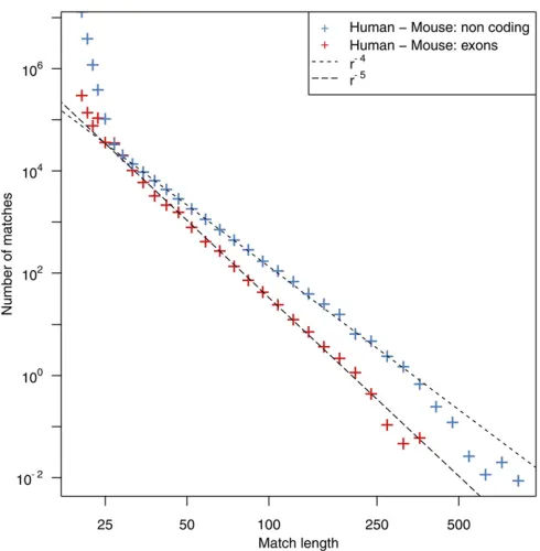
Computing the match length distribution (MLD) from the comparison of human and mouse genomes, we thus expect to observe much longer exact matches than in a comparison of two random sequences of the same lengths. The observed MLD for exons and noncoding sequences in the human and mouse RepeatMasked genomes is shown in Figure 1. At the left end of the distribution,i.e., forr,25 bp, the distribution is dominated by random matches, as described by Equation 1. As expected, this MLD deviates from the random model for matches.25 bp.

Interestingly, in this asymptotic regime, the MLD exhibits a power-law tail MðrÞ ra_{. In the comparison of exonic}

se-quences, the exponent ais close to –5, in contrast to the MLD of noncoding sequences, where the exponentais close to–4 (Gao and Miller 2011, 2014; Massipet al.2015). This property appears to be impressively reproducible in the com-parison of various pairs of species (see Supplemental Mate-rial, File S1, Figure S1). In all cases, the value of a was calculated using the maximum-likelihood estimator. To as-sess the robustness of this estimator, we also performed a bootstrap analysis that showed good agreement with the es-timated value ofa; seeMaterials and Methods. Note also that discrepancies of the power-law behavior can be observed for very long matches, since such matches are scarce and random noise distorts the distributions.

It is tempting to speculate that this peculiar behavior of exonic sequences is a direct consequence of their coding function. However, we demonstrate in the following that this distribution can be accounted for by a simple evolutionary model that takes into account the generation of paralogous sequences (due to segmental duplications) and orthologous sequences (due to speciation) (Fitch 2000). Further, we as-sume that paralogous and orthologous exact matches are subsequently broken down by random substitutions. These dynamics can be modeled by a well-known stick-breaking process (Kuhn 1930; Ziff and McGrady 1985) introduced below. Since our model describes the existence of long match-ing sequence segments in two genomes, it also has to include selection. However, we model selection in a minimal way, since we assume only that regional substitution rates are distributed, such that there are regions that evolve very slowly. Our model can therefore be viewed as a minimal model for evolution of functional sequences, which repro-duces certain statistical features of their score distributions. In the next section, we describe the main methods and the data analyzed in this article.

Materials and Methods

Computational and statistical analysis

Computing MLDs:Tofind all identical matches (both in the case of self and comparative alignments), we used the mummer pipeline (Kurtzet al.2004) (version 3.0), which allows us to find all maximal exact matches between a“query”and a refer-ence sequrefer-ence using a computationally efficient suffix tree ap-proach. For our analyses, we used the following options: -maxmatch such that mummer searches for all matches regard-less of their uniqueness; -n that states that only9A9,9T9,9C9, and

9G9can match; -b such that mummer searches for matches on both strands; and -l 20 tofilter out matches,20 bp.

The number of matches expected for a random i.i.d. se-quence grows quadratically with L. For instance, we expect 3.531016_{matches of length 2 in a comparison of two} se-quences of lengthL= 109_{bp (see Equation 1). For this} rea-son, we have to define a threshold for the length of matches that mummer should output especially when comparing en-tire eukaryotic genomes.

Logarithmic binning: Power laws appear in the tail of dis-tributions, meaning that they are associated to rare events, which are thus subject to strongfluctuations. The high impact of noise in the tail of the distribution can make the assessment of the exponent of the distribution difficult. A way to resolve

this issue is to increase the size of the bins with the value of the horizontal axes and normalize the data accordingly. Namely, the observed values for each bin are divided by the size of the bin. The most common choice to do this is known as the logarithmic binning procedure, which consists of increasing the size of the bin by a constant factor. Note that by doing so, we dramatically reduce the number of data points and some in-formation is lost as we aggregate different data points together in the same bin. Therefore it is often useful to consider both representations, with and without the logarithmic binning. See Newman (2005) for more details on the logarithmic binning procedure and on power-law distributions.

Estimating the value of the power-law exponent: To esti-mate the value of the exponent of the power-lawa, we com-pute the maximum-likelihood estimator. The estimatora^ is simply the value ofathat maximizes the log-likelihoodL,

L ¼Xn

i¼1

lnða21Þ2lnðxminÞaln

xi xmin

; (2)

such that

^

a¼ 212n

" Xn

i¼1 ln

xi xmin

#21

; (3)

while the value of xminhas to be determined visually. This estimator is also sometimes referred to as the Hill estimator (Hillet al.1975).

To estimate the robustness of the value of the exponents found using this method, we proceeded to bootstrap exper-iments on the human to mouse exome comparison. For each bootstrap, we sampled 5% of the mouse exons and compared them to all human exons. In each experiment, we calculated the exponent of the MLD, using the maximum-likelihood estimator as described in Newman (2005). We repeated this procedure 100 times. Values ofawere all in the range [–4.7,

–5.2] and the mean value for the exponent wasa=–4.9. Data availability

All genomes and their specific annotations (such as repeat elements and exons) were downloaded from the ensembl website (Cunninghamet al.2015), using the Perl API (version 80); the corresponding release of the human genome is GRCh38. In all cases, we downloaded the RepeatMasked ver-sions of genomes publicly available in the ensembl databases. Perl, R, and C++ scripts used to simulate the data and compute the match lentgh distributions are available athttps://

github.com/Flomass/MaLenDi. The MUMmer pipeline is freely

available online (http://mummer.sourceforge.net/).

Results

Theory

The stick-breaking model: Before we turn to the detailed description of our model, let us shortly introduce some relevant

results on random stick breaking. Consider a stick of lengthKat timet¼0;which will be sequentially broken at random posi-tions into a collection of smaller sticks. Breaks occur with ratem per unit length. The distribution of stick lengths at time t, denoted bymðr;tÞ;follows the integro-differential equation

@

@tmðr;tÞ ¼ 2m r mðr;tÞ þ2m

Z _N

r

mðs;tÞds (4) (Ziff and McGrady 1985; Massip and Arndt 2013), where thefirst term on the right-hand side represents the loss of sticks of lengthr due to any break in the given stick and the second term represents the gain of sticks of lengthrfrom the disruption of longer sticks. Note that for any stick of lengths.r;there are two possible positions at which a break would generate a stick of lengthr.

The initial state is one unbroken stick of length K; i.e., mðr;0Þ ¼dðK;rÞ:The corresponding time-dependent solution is

mðr;tÞ ¼

8 < :

2tþt2ðK2rÞexpð2trÞ for 0,r,K; expð2trÞ for r¼K;

0 otherwise

(5)

(Ziff and McGrady 1985), where we define the rescaled time t¼mt:Apart from the singularity atr=K, which accounts for the possibility that the stick is not even broken once, the distribution is dominated by an exponential function; i.e., there are far more small sticks than long ones. The average stick length is given bymðtÞ ¼K=t:

The match length distribution of evolving sequences:The above stick-breaking process can be used to describe the breakdown of a long DNA match into several smaller ones

by substitutions in either one of the two copies of the match. In a comparison of two species,AandB, long iden-tical segments are the signature of homology relation-ships between the two sequences. These homologous sequences either result from the copy of the genetic ma-terial during the time of speciation and are then ortholo-gous sequences (see the blue dashed line in Figure 2) or are due to segmental duplications in the ancestral ge-nome,i.e., paralogous sequences (see the red dashed line in Figure 2) (Fitch 2000).

The MLD is then given by the integral

MðrÞ ¼

Z _N

0

NðtÞmðr;tÞdt; (6) where NðtÞ is the number of homologous sequences with divergence t and mðr;tÞ is given in Equation 5; see also Massip et al.(2015). The divergence between a pair of orthologous sequences is the sum of two contributions t¼mA;i tspþmB_;i tsp;wheretspis the time since the two spe-cies diverged andiis an index for regions in the genomes. The regional mutation rates mA;iandmB;i in the two species are themselves distributed and assumed to be independent from each other. We therefore defineNABas

NABðtÞ ¼

Z _t

0

NAðtAÞNBðt2tAÞdtA; (7)

whereNAðtÞ[resp.NBðtÞ] is the number of sequences with divergence t from the last common ancestor Iin species A (resp. B). However, if the two regions are paralogous, the divergence t is a sum of three independent contributions t¼mA;itspþ ðmI_;iþmI;jÞtdupþmB_;jtsp; where tdup represents the time elapsed between the segmental duplication and the split of the two species. There are NAIBðtÞ paralogous sequences with divergencet;with

NAIBðtÞ ¼

Z _t

0 Z _t2tA

0

NAðtAÞNIðt2tA2tBÞNBðtBÞdtBdtA:

(8)

For our purposes we are not interested in the full functional form of the distributions in Equations 7 and 8 but have to consider only their behavior for small t/0; because long matches [and thus the tail of the distribution of the match length distributionM(r)] stem from homologous exons that exhibit a small divergence t. A more general discussion about the functional form of the distribution of pairwise distances can be found in Sheinmanet al.(2015). We there-fore take the Taylor expansion of the distributions N(t) aroundt¼0:Using Leibniz’s formula to take the derivative under the integral sign (Flanders 1973), wefind for orthol-ogous exons

NABðtÞ ¼NAð0ÞNBð0Þtþ O

t2 (9)

(see details in File S1) and subsequently the match length distribution

MABðrÞ ¼

Z _N

0

NABðtÞmðr;tÞdt

¼NAð0ÞNBð0Þ6K22r r4

NAð0ÞNBð0Þ

6K r4

(10)

(Massipet al.2015), asKr. In contrast, expanding Equa-tion 8 aroundt¼0finds

NAIBðtÞ ¼

1

2 NAð0ÞNIð0ÞNBð0Þt

2_{þ Ot}3 ₍₁₁₎

(see details inFile S1). Thus, for paralogous pairs, the num-ber of regions with divergencetincreases ast2in the smallt limit. Therefore the match length distribution exhibits a power-law tail with exponenta¼ 25;

MAIBðrÞ ¼

Z _N

0

NAIBðtÞmðr;tÞdt

¼NAð0ÞNIð0ÞNBð0Þ12K26r r5

NAð0ÞNIð0ÞNBð0Þ12K r5 ;

(12)

asKr.

Depending on the number of orthologous sequencesQortholog and paralogous sequencesQparalog;we will be able to distin-guish two regimes: one where the MLD follows ana¼ 24 power law and one where it follows ana¼ 25 power law. From Equations 10 and 12, it is straightforward tofind that the crossover pointrcbetween those regimes (see Figure 3) is at

rc¼2NIð0Þ: (13)

Recall thatNIð0Þis defined as the number of paralogous seg-ments that have not mutated even a single time since the duplication event at the time of the split. Thus, this term is proportional to the ratio of the duplication rate over the mutation rate. If NIð0Þ 10; there are significantly more

paralogous sequences compared to orthologous ones and the crossover value, rc; is large. Then, only the a¼ 25 power-law tail will be observed. On the other hand, if NIð0Þ 10; then the crossing point rc is expected to be ,20 such that the a¼ 25 power law holds only for lengths where the distribution is already dominated by ran-dom matches. In contrast to previous models (Massipet al. 2015), this model does take into account the contribution of paralogous sequences and can explain both power-law be-haviors and therefore predicts the crossing point between the two regimes.

Numerical validation

Our theoretical considerations predict a complex behavior of the match length distribution under the described evolution-ary dynamics. The key ingredients are segmental duplications, generating paralogous sequences in an ancestral genome, and point mutations that break identical pairs of homologous sequences of the two genomes into smaller pieces. To illustrate our theoretical predictions concerning the two power laws, as well as the existence of the crossover pointrc;we simu-lated the evolution of sequences according to the discussed scenario.

We describe the evolution of a genome of lengthL accord-ing to two simple processes, point mutations and segmental duplications. Point mutations exchange one base pair by an-other one and occur with ratemper base pair and unit of time. To mimic the existence of regions under different degrees of selective pressure, we allow for regional differences of the point mutation rates. Segmental duplications copy a contig-uous segment of Knucleotides to a new position where it replaces the same amount of nucleotides, such that the total

length of the genome stays constant. Segmental duplications occur with ratelper base pair.

Our simulation has two stages (see Figure 2). At timet= 0, we generate a random i.i.d. sequenceS:During a timet0;this sequence evolves according to the two described processes. In thisfirst stage, the mutation rate is the same for all posi-tions. At the end of this stage, the sequence represents the common ancestral genome of two species. At the beginning of the second stage, we copy the entire sequence of the common ancestor to generate the genomes of the two speciesAandB. These sequences are then subdivided intoMcontinuous re-gions of equal length. In each such regionj, the point muta-tion ratesmA;jðresp:mB;jÞare the same for all sitesiand are drawn from an exponential distribution with meanm(i.e., the point mutation rate during the first stage). We chose the exponential distribution because it stipulates the least infor-mation under the given constraints. For more details about the simulation procedure, seeFile S1, Appendix A.

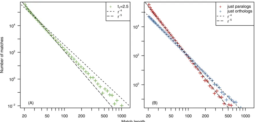
We show the result of the comparison of simulated se-quences in Figure 4, left. We obtain a power-law tail in the match length distribution, which for match length 20,r,100 has an exponent a¼ 25 and an exponent a¼ 24 for longer matches r.100: For simulated se-quences, we can easily classify homologous sequences into orthologous and paralogous sequences (while for natural se-quences, paralogs and orthologs are not easily distinguish-able due to genomic rearrangements). We show the MLD obtained from the comparison of paralogs and the MLD obtained from the comparison of orthologs for simulated sequences in Figure 4, right. We can clearly observe that orthologous sequences generate ana¼ 24 power-law dis-tribution while paralogous matches generate an a¼ 25

power-law distribution. We can further easily identify the crossing pointrcas the value ofrfor which we obtain more matches from the comparison of orthologs than from the comparison of paralogs.

In the previous section the value of this crossing point between the two regimes was predicted to be rc¼2NIð0Þ (see Equation 13), whereNIð0Þis the number of paralogous segments with a divergence t¼0 just before the species split. In our simulation procedure,NIð0Þis simply the num-ber of sequences that have been duplicated but that have not been mutated yet at the splitting timet¼t0:This num-ber is known to beNIð0Þ ¼lL=mΚ(Massip and Arndt 2013). In our simulations,l¼0:05;m¼1;K¼1000;andL¼107 and therefore we predictrc¼100;which is in good agree-ment with our observations in Figure 4. The results of our simulations are thus in good agreement with our analytical predictions.

Discussion

We developed a simple model that accounts for power-law tails in the length distribution of exact matches between two genomes. Our model assumes regional differences of the selective pressure such that the substitution rates in a region are drawn from a certain distribution. However, for naturally evolving exons the selective pressure varies also on shorter length scales. For instance, some nucleotides for many codons can be synonymously substituted by another one, mostly at third codon positions. Therefore,

these substitutions at third codon positions occur with a higher rate than nonsynonymous ones. Hence, exons are expected to break preferentially at positions 3n, withn2ℕ; such that the matches with 100% identity would have lengths 3nþ2 with integern:Classifying genomic matches according to the remainder that is left when dividing their length by 3, we observe an almost 10-fold overrepresen-tation of matches with length 3nþ2 over matches of lengths 3n and 3nþ1; see Figure 5. This suggests that the match-breaking process is dominated by the synony-mous mutation rate

Using the presented model, the puzzling observation of an a¼ 24 power-law tail in the MLD in the comparison of the human and mouse genomes and a corresponding a¼ 25 power-law tail in the comparison of their exomes can be explained. Although the sequences stem from the same spe-cies, the relative amount of paralogous to orthologous se-quence segments is different in the two data sets, which subsequently leads to different crossover points rc:Because of the selective pressure on coding exons, the number of non-mutated paralogous sequences at the time of species diver-genceNIð0Þis higher (relative to the number of orthologous sequences) in the exonic data set than in the noncoding data set. Thus, the crossover point in exomesrcis larger than the longest observed match and only thea¼ 25 power law can be observed.

The opposite is true for matches in the alignment of noncoding sequences. Quantitatively, in this set, paralogous sequences play a lesser role and therefore only thea¼ 24 power law is observed (see Figure 1). This is surprising, as the duplication rate is thought to be roughly the same in the coding and noncoding parts of genomes. To confirm this paradoxical observation, we classified matches according to the uniqueness of their sequences in both genomes. As-suming that unique matches are more likely to be ortholo-gous, this gives us a rough classification of homologs into orthologs and paralogs, although matches unique in both sequences can be paralogs. After the classification of all matches, our analysis made apparent that matches unique in both genomes dominate the MLD in the comparison of the noncoding parts of the genomes, while matches with several occurrences in either (or both) of the genomes dom-inate the distribution in the case of the comparison of exomes (see File S1, Figure S2). Moreover, we computed the MLD from the set of nonunique matches of the noncod-ing part of the genomes. In this comparison, the contribu-tion of paralogs is expected to be much higher than in the full set. As expected, this MLD also exhibits an a¼ 25 power law (see File S1, Figure S2), confirming that the relative contribution of orthologs and paralogs is respon-sible for the shape of the MLD. These differences in the proportion of paralogous sequences in the coding and noncoding DNA are likely due to the fact that paralogs are more often retained in the coding part than in the coding part of genomes. Since there are many more non-coding sequences in both genomes, we also observe at least

Figure 5 The MLD computed from the comparison of the human and the mouse exome, represented without logarithmic binning. Three differ-ent colors are used to represdiffer-ent matches of length 3n; 3nþ1; and 3nþ2:Dashed lines represent power-law distribution with exponents

10 times more matches in the comparison of noncoding sequences than in the comparison of exomes.

The presented model does not account for changes in the divergence rates after a duplication, a phenomenon that is well documented following a gene duplication (Scannell and Wolfe 2008; Han et al. 2009; Panchin et al. 2010; Pegueroleset al. 2013). To assess the impact of this phe-nomenon on the MLD, we performed simulations where the two paralogous segments are assigned different and independent mutation rates. Interestingly, these simula-tions yield results qualitatively similar to those of the sim-pler model introduced above (seeFile S1, Figure S3). This new condition does not affect the value of the number of paralogous sequences that have not diverged at the time of the split [i.e., the value ofNj(0)] and thus the shape of the distribution.

The model we present is very simple, and more realistic models of genome evolution include many more evolutionary processes (Dalquen et al.2012). For instance, we could in-clude a transition/transversion bias in the mutational pro-cess, variations of mutation rates in time, a codon usage bias, or different rates of duplication within and between chromosomes. Since in the end we consider just identical matching sequences and want to explain the power-law tail in the MLD, all these additional model details are not expected to affect the results.

In this article, we demonstrate that on the genome-wide scale, the length distribution of identical homologous se-quence segments in a comparative alignment is nontrivial and exhibits a power-law tail, and we propose a simple model able to explain such distributions. While paralogous se-quences, which had been duplicated before the species di-verged, generate a power-law tail with exponenta¼ 25; orthologous sequences generate a power-law tail with expo-nenta¼ 24:Depending on the relative amount of paralo-gous to ortholoparalo-gous sequences there is a crossover between these two law regimes. The exponent of the power-law tail in the comparative MLD can therefore be a litmus test for the abundance of paralogous relative to orthologous se-quences, while it is usually difficult to distinguish between orthologous and paralogous sequences using classical bio-informatic methods (Studer and Robinson-Rechavi 2009; Dalquenet al.2013; Gabaldón and Koonin 2013). If paralo-gous sequences dominate, the crossover occurs for a large value ofrand the apparent exponent is equal to25; other-wise it is equal to24:

Our method is very easy to apply. In particular, it does not require that genomes are fully assembled as long as the continuous sequences are.1 kbp, comparable to the longest matches one expects. A natural extension of our method would be to apply it to sequences from metagenomic samples to assess relative amounts of paralogous and orthologous sequences. However, we would also have to consider hori-zontal gene transfer, which is common among prokaryotes and generates homologous sequence segments even between unrelated genomes. Our computational model can easily be

extended to take into account these and other more complex biological processes, using, for instance, already developed tools (Dalquenet al.2012). This would allow us to assess their impact on our results and will be the subject of future work.

This study shows that even very simple models can often successfully be applied to seemingly very complex phenomena in biology. We were able to present a minimal model for the evolution of homologous sequences that includes effects due to segmental duplications and evolution under selective constraints—the two processes that are responsible for a power-law tail in the length distribution of identical match-ing sequences.

Literature Cited

Altschul, S. F., W. Gish, W. Miller, E. W. Myers, and D. J. Lipman,

1990 Basic local alignment search tool. J. Mol. Biol. 215: 403–

410.

Bejerano, G., M. Pheasant, I. Makunin, S. Stephen, W. J. Kentet al.,

2004 Ultraconserved elements in the human genome. Science

304: 1321–1325.

Cunningham, F., M. R. Amode, D. Barrell, K. Beal, K. Billiset al.,

2015 Ensembl 2015. Nucleic Acids Res. 43: D662–D669.

Dalquen, D. A., M. Anisimova, G. H. Gonnet, and C. Dessimoz,

2012 Alf—a simulation framework for genome evolution.

Mol. Biol. Evol. 29: 1115–1123.

Dalquen, D. A., A. M. Altenhoff, G. H. Gonnet, and C. Dessimoz,

2013 The impact of gene duplication, insertion, deletion,

lat-eral gene transfer and sequencing error on orthology inference: a simulation study. PLoS One 8: e56925.

Fitch, W. M., 2000 Homology: a personal view on some of the

problems. Trends Genet. 16: 227_–231.

Flanders, H., 1973 Differentiation under the integral sign. Am.

Math. Mon. 80: 615_–627.

Gabaldón, T., and E. V. Koonin, 2013 Functional and evolutionary

implications of gene orthology. Nat. Rev. Genet. 14: 360–366.

Gao, K., and J. Miller, 2011 Algebraic distribution of segmental

duplication lengths in whole-genome sequence self-alignments. PLoS One 6: e18464.

Gao, K., and J. Miller, 2014 Human–chimpanzee alignment:

or-tholog exponentials and paralog power laws. Comput. Biol.

Chem. 53: 59–70.

Han, M. V., J. P. Demuth, C. L. McGrath, C. Casola, and M. W.

Hahn, 2009 Adaptive evolution of young gene duplicates in

mammals. Genome Res. 19: 859_–867.

Hill, B. M., 1975 A simple general approach to inference about

the tail of a distribution. Ann. Stat. 3: 1163_–1174.

Kuhn, W., 1930 Über die Kinetik des Abbaues hochmolekularer

Ketten. Ber. Dtsch. Chem. Ges. 63: 1502_–1509.

Kurtz, S., A. Phillippy, A. L. Delcher, M. Smoot, M. Shumwayet al.,

2004 Versatile and open software for comparing large

ge-nomes. Genome Biol. 5: R12.

Massip, F., and P. F. Arndt, 2013 Neutral evolution of duplicated

DNA: an evolutionary stick-breaking process causes scale-invariant behavior. Phys. Rev. Lett. 110: 148101.

Massip, F., M. Sheinman, S. Schbath, and P. F. Arndt, 2015 How

evolution of genomes is reflected in exact DNA sequence match

statistics. Mol. Biol. Evol. 32: 524–535.

Needleman, S. B., and C. D. Wunsch, 1970 A general method

applicable to the search for similarities in the amino acid

se-quence of two proteins. J. Mol. Biol. 48: 443_–453.

Newman, M. E., 2005 Power laws, pareto distributions and zipf_’s

Panchin, A. Y., M. S. Gelfand, V. E. Ramensky, and I. I. Artamonova,

2010 Asymmetric and non-uniform evolution of recently

du-plicated human genes. Biol. Direct 5: 54.

Pegueroles, C., S. Laurie, and M. M. Albà, 2013 Accelerated

evo-lution after gene duplication: a time-dependent process

affect-ing just one copy. Mol. Biol. Evol. 30: 1830–1842.

Salerno, W., P. Havlak, and J. Miller, 2006 Scale-invariant

struc-ture of strongly conserved sequence in genomic intersections

and alignments. Proc. Natl. Acad. Sci. USA 103: 13121–13125.

Scannell, D. R., and K. H. Wolfe, 2008 A burst of protein sequence

evolution and a prolonged period of asymmetric evolution

fol-low gene duplication in yeast. Genome Res. 18: 137_–147.

Sheinman, M., F. Massip, and P. F. Arndt, 2015 Statistical

prop-erties of pairwise distances between leaves on a random yule tree. PLoS One 10: e0120206.

Smith, T. F., and M. S. Waterman, 1981 Identi_fication of common

molecular subsequences. J. Mol. Biol. 147: 195–197.

Studer, R. A., and M. Robinson-Rechavi, 2009 How confident can

we be that orthologs are similar, but paralogs differ? Trends

Genet. 25: 210–216.

Ziff, R. M., and E. D. McGrady, 1985 The kinetics of cluster

frag-mentation and depolymerisation. J. Phys. Math. Gen. 18: 3027.

Appendix A: Simulating the Evolution of DNA Sequences

397

To simulate our evolutionary models, we proceeded as follows. A sequence of nucleotides

398

S

= (

s

1

, . . . , s

L

)

of length

L

with

s

i

∈ {

A

,

C

,

G

,

T

}

is evolved through time in small time

399

intervals

∆

t

. The time intervals

∆

t

are small enough such that for all considered evolutionary

400

processes

E

of our model, which are assumed to occur with rate

ρ

E

, we have

ρ

E

L

∆

t

1

.

401

At each step, random numbers

u

E

i

for all positions

i

and possible evolutionary processes

E

402

are drawn from a uniform distribution. The event

E

then occurs at position

i

if

u

E

i

< ρ

E

∆

t

.

403

These steps are repeated until the desired time

t

has elapsed.

404

Sequences evolve according to two simple processes, point mutations and segmental

du-405

plications. Point mutations exchange one nucleotide by another and occur with rate

µ

per

406

bp and unit of time. Note that to mimic the existence of regions under different degrees of

407

selective pressure we allow for regional differences of the point mutation rates. Segmental

408

duplications copy a contiguous segment of

K

nucleotides starting at position

c

and paste

409

them to a different position

v

, such that the

K

nucleotides at positions

v

to

v

+

K

−

1

are

410

replaced by the ones from position

c

to

c

+

K

−

1

. As a consequence, the total length of

411

the sequence

L

stays constant in time. The segmental duplication process occurs with rate

412

λ

per bp and per unit of time.

413

The evolutionary scenario of our simulation has two stages, as shown in Fig. 2. At time

414

t

= 0

, we start with a random iid sequence

S

with equal proportions of all 4 nucleotides.

415

During a time interval of length

t

0

, this sequence evolves according to the two described

416

processes. In this first stage, the mutation rate is the same for all positions. At the end of

417

this stage, the sequence represents the common ancestor of the two species.

418

At the beginning of the second stage, we duplicate the entire sequence of the common

419

ancestor to generate the genomes of the two species

A

and

B

. These sequences are then

420

subdivided into

M

continuous regions of equal lengths. The point mutation rates

µ

A,j

(resp.

421

µ

B,j

) are the same for all sites in a given region

j

and are independently drawn from the

422

same exponential distribution of mean

µ

, i.e. the point mutation rate during the first stage.

423

For simplicity, the length of the

M

continuous regions is set to

M

=

K

and the segmental

424

duplication rates in both species

λ

during the second stage are set to zero. Both species then

425

evolve independently for a divergence time

t

sp

, and we compute the MLD from a comparison

426

of the sequences of the two species

A

and

B

. Note that even when we chose finite duplication

rates after the split (i.e.

λ >

0

in the second stage), we obtained qualitatively similar MLDs.

428

To control for the potential impact of our choice to keep the genome size constant on our

429

results, we also simulated the evolution of sequences where duplicated segments where added

430

to the sequences (thus generating growing genomes). In that case, duplicates were added

431

at the very end of the sequence, such that duplicates do not disrupt pre-existing matches.

432

This control experiment yields qualitative similar results, in agreement with our theoretical

433

considerations (data not shown).

434

Appendix B: Calculation of the derivative of

N

AIB 435

In this section we describe the Taylor expansion that leads to Eq. (11) from the main

436

text. The Taylor expansion for

N

AIB

in the neighborhood of

τ

= 0

results in

437

N

AIB

=

N

AIB

(0) +

N

AIB0

(0)

τ

+

N

00 AIB

(0)

τ

2

2

+

N

000 AIB

(0)

τ

3

6

+

O

(

τ

4

₎

_.

(S1)

From Eq. (8) in the main text, it follows that the first term always vanishes. Using

438

Leibniz formula to take the derivative under the integral sign in Eq. (8), we find for the first

439

derivative

440

N

_AIB0

(

τ

) =

ˆ

τ

0

ˆ

τ2

0

N

B

(

τ

B

)

N

A

(

τ

2

−

τ

B

)

N

I0

(

τ

−

τ

2

)

dτ

B

dτ

2

+

ˆ

τ

0

N

I

(0)

N

B

(

τ

B

)

N

A

(

τ

−

τ

B

)

dτ

B

.

(S2)

It follows that the first derivative of

N

AIB

(

τ

)

at

τ

= 0

vanishes. For the next term, we get

441

N

_AIB00

(

τ

) =

N

A

(0)

N

I

(0)

N

B

(

τ

)

(S3)

+

ˆ

τ

0

N

I

(0)

N

B

(

τ

B

)

N

A0

(

τ

−

τ

B

)

dτ

B

+

ˆ

τ

0

ˆ

τ2

0

N

B

(

τ

B

)

N

A

(

τ

2

−

τ

B

)

N

I00

(

τ

−

τ

2

)

dτ

B

dτ

2

+

ˆ

τ

0

N

B

(

τ

B

)

N

I0

(0)

N

A

(

τ

−

τ

B

)

dτ

B

+

N

A

(0)

N

I

(0)

N

B

(

τ

)

.

(S4)

Here, all terms but the first one vanish for

τ

= 0

. Similarly, we can calculate the third

442

derivative of

N

(

τ

)

, and we find that for

τ

= 0

443

such that Eq. (S1) finally takes the form

444

N

AIB

(

τ

) =

1

2

N

A

(0)

N

B

(0)

N

I

(0)

τ

2

+

1

6

(

N

0

A

(0)

N

B

(0)

N

I

(0) +

N

A

(0)

N

B0

(0)

N

I

(0) +

N

A

(0)

N

B

(0)

N

I0

(0))

τ

3

+

O

(

τ

4

)

.

(S6)

Therefore, as long as

445

τ

3

N

A

(0)

N

B

(0)

N

I

(0)

N

_A0

(0)

N

B

(0)

N

I

(0) +

N

A

(0)

N

_B0

(0)

N

I

(0) +

N

A

(0)

N

B

(0)

N

_I0

(0)

,

(S7)

N

AIB

(

τ

)

is expected to scale as

τ

2

and subsequently

M

(

r

)

∼

r

−5

.

+

+

++

++

++

₊

++

₊₊

+++

++++++

₊₊₊₊₊

++++

₊₊₊

+++

++

+

Match length

Number of matches

25 50 100 200 500

102 104

+ Human Chimp r−4

r−5

(A)

+

+++

+++

+++

₊₊

++

+++

₊

++

+++

+++

+++

++

+

++

25 50 100 200

100 102 104

+ Mouse Rabbit r−4

r−5

(B)

25 50 100 200

100 102 104

+

+

++

++

+

+++

++

++

++

++

+++

++

++

+++

+

+ Human Turkey

r−4 r−5

(C)

25 50 100 200

100 102 104

+

+

++

+

+

+

+

+

+

++

+

+

+

+

++

+

+ Human Zebrafish r−4

r−5

(D)

Figure S1. MLDs computed from the comparison of the exome of several species. In all four

panels, dashed lines represent power-law distribution with exponent

α

=

−4

and

α

=

−5

, and

empirical data are represented using logarithmic binning. MLDs represented are computed from

the comparison of the exomes of (A) Human and Chimp, (B) Mouse and Rabbit (C) Human and

+

+

+

+

+

+

+

+

+

+

+

+

+

+

+

+

+

+

+ +

+

+

+

+

+

+

+

+

+

+

+

+

+

+

+

+

+

+

+

+

+

+

+

+

+

+

+

+

+

+

+ +

+

+

+ +

Match length

Number of matches

20 50 100 200

100 102 104 106

+

+

Multiple matches Unique Matches r−4

r−5

Figure S2. MLD computed from the comparison of subsets of the non-coding part of Human and

Mouse genomes. Also the non-coding part of these genomes contains paralogous sequence segments

from segmental duplications before the species split. To enrich for such sequences we partitioned

the genomes into two subsets. Using self-alignments of the two species, we first created two libraries

containing the sequences of all exact matches within their non-coding part. This library is thus be

enriched for sequences duplicated before and after the speciation. Subsequently the two libraries are

compared and their MLD (multiple matches, red data points) shows the expected

−5

power-law.

As a control, the complements of the two libraries show an

−4

power-law (unique matches, blue

+++

₊₊₊₊

+++

₊₊

++

++

₊₊

++

++

++

++

++

++

₊₊

++

₊₊

+

++

+++

++

++++

Match length

Number of matches

20 50 100 200 500 1000 2000

100

102

104

+ t1=2.5

r−4 r−5

(A)

++

+++++

+++

₊₊

++

++

++

++

++

++

++

++

+++

++

++

+

++

₊

++

+

₊

++++++

₊₊₊₊

+++

+++

+++

₊₊

++

+++

₊₊

++

+++

+++

₊

++

+++++

+

+++

20 50 100 200 500 1000

10−2

100

102

104

+

+

just paralogs just orthologs r−4

r−5

(B)

Figure S3. The MLD computed from

1000

simulated sequences according to the procedure described

in the main text, but in this case, after any duplication event, the two copies are randomly assigned

a new mutation rate, drawn from the mutation rate distribution (i.e. an exponential distribution

of mean

1

). Data are represented using the logarithmic binning. On the left panel, we show the

MLD generated computed from all possible matches, while on the right panel, we represent two

different MLDs: one computed from paralogous matches only (red), and one computed from the

orthologous matches only (blue). One can see that the results of these simulations hold qualitatively