REED, JAMES ALLEN. A Low Rank Approach to Computing Derivatives Using Automatic Differentiation. (Under the direction of Hany S. Abdel-Khalik).
This manuscript outlines a new approach for increasing the efficiency of applying automatic
differentiation (AD) to large scale computational models. By using the principles of the
Efficient Subspace Method (ESM), low rank approximations of the derivatives for first and
higher orders can be calculated using minimized computational resources. The output
obtained from nuclear reactor calculations typically has a much smaller numerical rank
compared to the number of inputs and outputs. This rank deficiency can be exploited to
reduce the number of derivatives that need to be calculated using AD. The effective rank can
be determined according to ESM by computing derivatives with AD at random inputs.
Reduced or pseudo variables are then defined and new derivatives are calculated with respect
to the pseudo variables. Two different AD packages are used: OpenAD and Rapsodia.
OpenAD is used to determine the effective rank and the subspace that contains the
derivatives. Rapsodia is then used to calculate derivatives with respect to the pseudo
variables for the desired order. The overall approach is applied to a few simple mathematical
© Copyright 2012 by James Allen Reed
by
James Allen Reed
A thesis submitted to the Graduate Faculty of North Carolina State University
in partial fulfillment of the requirements for the degree of
Master of Science
Nuclear Engineering
Raleigh, North Carolina
2012
APPROVED BY:
_______________________________ ______________________________
Steven Campbell Paul Hovland
BIOGRAPHY
James A. Reed was born on October 18th 1987 in Beaver, Pennsylvania. He attended Penn State University in State College, PA from 2006 to 2010 where he obtained Bachelor of
Science degrees in Nuclear and Mechanical Engineering with honors in Nuclear Engineering.
Upon graduation from Penn State, he continued his studies in Nuclear Engineering at North
Carolina State University in Raleigh. While at NCSU, he started working on using automatic
differentiation as a means to calculate derivatives from nuclear reactor codes for use in
sensitivity analysis and uncertainty quantification. He collaborated with the Mathematics
and Computer Science Division at Argonne National Laboratory and the work performed is
ACKNOWLEDGMENTS
I would first like to thank my parents for their support. Without them, I would not
have any chance to be in the position that I am today. I would also like to thank Dr.
Abdel-Khalik for his guidance and for allowing me the opportunity to work under him at North
Carolina State University. I must also thank Paul Hovland for sponsoring me during the
summer at Argonne National Laboratory where essential work for this project was
completed. I very grateful for the assistance I received from Jean Utke while at Argonne.
Without his work on OpenAD and Rapsodia, none of this would be possible. Last but
certainly not least, I am dearly thankful for the love and support from Casandra Niebel, who
TABLE OF CONTENTS
LIST OF TABLES ... vi
LIST OF FIGURES ... vii
CHAPTER 1 Introduction ... 1
1.1 Applications of Automatic Differentiation ... 1
1.2 Uses of Derivatives ... 1
1.3 Problem Reduction via the Efficient Subspace Method ... 4
1.4 Multi-scale Phenomena Modeling ... 5
1.5 Thesis Contents ... 6
CHAPTER 2 Computational Methods ... 8
2.1 AD Theory ... 8
2.1.1 Forward Mode ... 12
2.1.2 Reverse Mode ... 14
2.1.3 Active Variables... 15
2.2 OpenAD ... 16
2.3 Rapsodia ... 16
2.4 Efficient Subspace Method ... 18
2.5 General Methodology ... 20
CHAPTER 3 Implementation... 26
3.1 Implementation on a General FORTAN Code ... 26
CHAPTER 4 Examples and Test Cases ... 32
4.1 Two-minute AD Examples ... 32
4.1.1 OpenAD/F Example... 32
4.1.2 Rapsodia Example ... 36
4.2 Matrix-Vector Product Example ... 41
4.3 Scalar-valued Model Example ... 48
4.4 Vector-valued Model Example ... 53
4.5 Important Directions ... 56
4.6 Third Order function Approximated with Second Order derivatives ... 62
5.1 Conclusions ... 72
LIST OF TABLES
Table 2-1: Evaluation Trace for Equation (4) ... 10
Table 2-2: Forward mode evaluation trace ... 13
Table 2-3: Reverse mode evaluation trace ... 17
Table 4-1: Results for the scalar-valued model example ... 52
Table 4-2: Results for the vector-valued model example ... 55
Table 4-3: Error criterion evaluations with random orthogonal inputs ... 61
Table 4-4: Error criterion evaluations with random inputs ... 61
Table 4-5: Surrogate model error evaluation around one point ... 64
LIST OF FIGURES
Figure 2.1: Computation Graph of Table 2-1 ... 11
Figure 4.1: Simple subroutine for ‘Two-minute’ forward OpenAD example ... 33
Figure 4.2: Main program used in the ‘Two-minute’ forward OpenAD example... 33
Figure 4.3: Output for the ‘Two-minute’ forward OpenAD example ... 35
Figure 4.4: Makefile contents for compiling and linking the ‘Two-minute’ forward OpenAD example... 35
Figure 4.5: Example reverse mode main program ... 37
Figure 4.6: Reverse mode example output ... 37
Figure 4.7: Rapsodia prepped subroutine for the ‘Two-minute’ example ... 37
Figure 4.8: Main program for the ‘Two-minute’ Rapsodia example... 39
Figure 4.9: Makefile contents for compiling and linking the ‘Two-minute’ Rapsodia example (first order) ... 40
Figure 4.10: Rapsodia example first order results ... 42
Figure 4.11: Rapsodia example second order results ... 42
Figure 4.12: Rapsodia example third order results ... 43
Figure 4.13: Matrix-vector product code with pseudo response definition ... 45
Figure 4.14: Matrix-vector product code with pseudo input definition ... 45
Figure 4.15: Singular value distribution for the matrix-vector product example ... 47
Figure 4.16: Python script used for the scalar-valued model example ... 50
Figure 4.17: Vector projection onto a plane ... 57
Figure 4.18: Graphical representation of the problem directions with the possible sampling areas indicated ... 60
Figure 4.19: Second order surrogate model plotted with actual function ... 65
Figure 4.20: Fuel temperature for variations of the axial expansion reactivity coefficient .... 67
Figure 4.21: Fuel temperature for variations of the Doppler reactivity coefficient ... 67
Figure 4.22: Fuel temperature for variations of the coolant reactivity coefficient ... 68
Figure 4.23: Fuel temperature for variations of the control rod expansion reactivity coefficient ... 68
CHAPTER 1
Introduction
1.1
Applications of Automatic Differentiation
Because detailed nuclear reactor calculations involve large input and output streams,
calculating derivative information can be a very time consuming task. Derivative
information is required for many aspects of nuclear engineering and analysis, such as
sensitivity analysis, design optimization, code-based uncertainty propagation, and data
assimilation. One tool that can be used to facilitate the calculation of derivatives is automatic
differentiation (AD) software. AD is a technique to reinterpret or completely transform a
computer program implementing a numerical model with the goal to calculate the derivatives
of specified output variables of the model with respect to specified input variables. The
principal method of AD is the application of the chain rule to the given elemental
decomposition of a mathematical function [1]. With continuing advances in computer
power, the application of AD is becoming a more feasible and attractive option for the
calculation of accurate derivatives [2] [3].
1.2
Uses of Derivatives
Derivative information is essential to sensitivity analysis, uncertainty quantification,
quantification can utilize model parameter sensitivities to estimate the potential error in
outputs in order to validate model. Derivatives are used in design optimization problems in
order to effectively tweak design parameters to obtain optimal performance. Data
assimilation uses derivatives for statistical interpolation of given data in order to estimate the
state of a given system. Surrogate modeling requires derivatives in order to build an
approximate model of a system via a truncated Taylor expansion.
The means of obtaining the full derivatives that populate the Jacobian matrix for a
sufficient number of model operating points is a very time and resource consuming task. AD
can be used to obtain the derivative values to within machine precision. Other possible
methods that are used for obtaining derivatives from computer codes of engineering models
involve hand-coding derivatives and using finite differences, but some of the more advanced
methods are the Generalized Perturbation Method and the Adjoint Method [4]. These
methods generally allow the computer code to be run faster than the corresponding AD
versions of the code, but the accuracy is generally lower and there is more room for error.
Therefore, it is desirable to enhance the efficiency of using AD and maintain acceptable
accuracy.
Two software package options for AD are OpenAD (www.mcs.anl.gov/OpenAD) and
Rapsodia (www.mcs.anl.gov/Rapsodia). In OpenAD, the derivative evaluation is performed
by a program resulting from the analysis and transformation of the original program that
implements the mathematical function or model of interest [4]. While OpenAD relies on
overloading as the vehicle of attaching derivative computations to the elementary operations
provided by the programming language such as the arithmetic operators and intrinsic
functions sin(x), exp(x), and so forth [5]. In our context, we use OpenAD with the so-called
reverse mode providing for the efficient computation of gradients with respect to a large
number of inputs. In contrast, Rapsodia implements higher order derivative computation in
forward mode. It is normally efficient for a small number of input variables and the
overloading overhead becomes negligible with higher derivative order. Both approaches are,
in principle, capable of calculating higher order derivatives. Higher-order derivatives with
source transformation by repeated application of the transformation tool increases complexity
of the tool and the program size and has not been shown to yield large benefits when
compared to operator overloading keeping in mind the expected small number of input
variables.
In nuclear engineering, derivatives are mainly used for the purposes of sensitivity
analysis and uncertainty quantification. Computational methods and uncertainties in input
data are the main limitation of the calculations necessary to design nuclear reactor systems.
Sensitivity analysis is often used to analyze the nuclear fuel cycle and the behavior of the
fuel. In analyzing a nuclear fuel rod, the sensitivities of key variables (fuel centerline
temperature, fission gas release, clad stress, etc.) to input parameters are found to be highly
non-intuitive and strongly dependent on the fuel-clad gap status and the history of the fuel
interest could be the neutron flux, fuel temperature, moderator temperature, and void fraction
at thousands of points throughout the reactor. The inputs of interest could be the complete
set of neutron cross sections that quantify the probabilities of different reactions taking place
in each type of material. It is easy to see that as the dimensions and details of the
calculations increase, the number of derivatives increases as well. The increase in the
number of higher order derivatives grows exponentially. For typical nuclear reactor
calculations, the number of inputs n and outputs m are on the orders of 6
10 and 5
10 ,
respectively. The numerical rank r of these problems is often orders of magnitude smaller
than the size of the input and output data streams with r typically around 2
10 [7]. This fact
can be used to reduce the effective dimensions of the problem and lessen the computational
time and storage requirements.
1.3
Problem Reduction via the Efficient Subspace Method
The mathematical theory of efficient subspace methods (ESM) recognizes that the
design and/or analysis of an engineering system is often judged by a few macroscopic
metrics that capture the overall behavior of the system [8]. ESM exploits the ill-conditioning
of the Jacobian matrix to reduce the number of code runs of the forward and reverse modes
of AD to a minimum [7]. ESM utilizes various properties from linear algebra including
orthogonality and the singular value decomposition (SVD) in order to identify the minimum
information necessary to represent the overall response of the system. It can be shown by
contribute much to the overall behavior of the system relative to other inputs. These
variables are deemed to be not as important, and by identifying them through ESM, their
place in the overall analysis can be lessened or ignored in order to focus on the more
important quantities and still capture the overall behavior of the system.
An example that illustrates the ideas behind ESM is in calculus for an integral
quantity such as distance via velocity profiles. The same distance can be obtained by
integrating different velocity profiles. Therefore, the question becomes “how can one
identify the required modeling changes associated with the different physics that will lead to
more accurate estimation of the macroscopic metrics of interest?” rather than “how can one
enhance the accuracy of the different field solutions [8]?”
1.4
Multi-scale Phenomena Modeling
The large rank reduction that can be obtained in some reactor calculations is a result
of the multi-scale phenomena modeling (MSP) strategy on which nuclear reactor calculations
are based. Besides nuclear reactor calculations, many other engineering systems involve
large variations in both time and length scales and are examples of applications of MSP. In
fact, many of today’s important engineering and physical phenomena are modeled via MSP,
e.g. weather forecast, geophysics, materials simulation [7]. To accurately model the large
time and scale variations, MSP utilizes a series of models varying in complexity and
coupled with low resolution (LR) macroscopic models to directly calculate the macroscopic
system behavior, which is often of interest to system designers, operators, and
experimentalists. The coupling between the different models results in a gradual reduction in
problem dimensionality thus creating large degrees of correlations between different data in
the input and output (I/O) data streams. ESM exploits this situation by treating the I/O data
in a collective manner in search of the independent pieces of information. The term ‘Degree
of Freedom’ (DOF), adopted in many other engineering fields, is used to denote an
independent piece of information in the I/O stream. An active DOF denotes a DOF that is
transferred from a higher to a lower resolution model, and an inactive DOF denotes a DOF
that is thrown out. ESM replaces the original I/O data streams by their corresponding active
DOFs. The number of active DOFs can be related to the numerical rank of the Jacobian
matrix.
1.5
Thesis Contents
This manuscript presents a method for using OpenAD and Rapsodia to efficiently
calculate first and higher order derivatives by reducing the size of the input stream according
to the efficient subspace method (ESM). Chapter 2 of this work describes the computational
methods and theory behind AD and the application of ESM. Chapter 3 presents a
generalized description of how this approach can be applied to a computational model.
Chapter 4 presents some simple examples of using the method as well as the results of
combines the SAS4A/SASSYS computer code with a simplified representation of the reactor
CHAPTER 2
Computational Methods
2.1
AD Theory
The quick, easy, intuitive (but inaccurate) way to calculate derivatives is by using a
finite difference or divided difference approach. The first order derivative for a function
is given by:
(1)
This method requires very small values of h in order to obtain useful results. Automatic (or
algorithmic) differentiation instead relies on the exact analytical expressions of the
derivatives for the basic functions ( ) that make up the overall function in
question. The chain rule of differentiation is used in order to follow the differentiation
calculation through the basic functions of the program. Equation (2) gives the chain rule for
a function f that is a function of another function g which is a function of x. Thus, f is
ultimately a function of x itself.
(2)
Equation (3) gives the chain rule in the case when and .
(3)
To show how the chain rule is used in AD, consider the following the example.
(4)
A computer will calculate y from and in much the same way that a human being would
go about doing it by hand. Intermediate values will be calculated for the lowest level
sub-functions (such as in this case), and then the values for these sub-functions will be
used to calculate the values for higher level functions (
). This process is continued until the overall value for the function is computed. Most
AD software packages follow this same control flow that is referred to as an evaluation trace.
An evaluation trace is basically a record of a particular run of a given program, with
particular specified values for the input variables, showing the sequence of floating point
values calculated by a (slightly idealized) processor and the operations that computed them
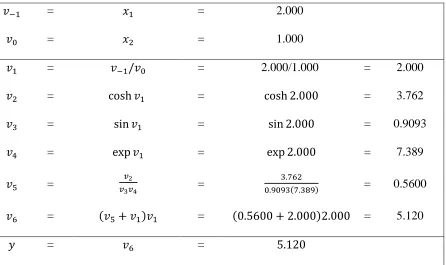
[1]. Table 2-1 shows an evaluation trace for Equation (4).
The intermediate mathematic variables are different from normal program
variables as they can normally not be assigned a value more than once [1]. A real computer
program that models an actual engineering system will contain functions that are much more
complex and have many more intermediates than the one given by Equation (4). To
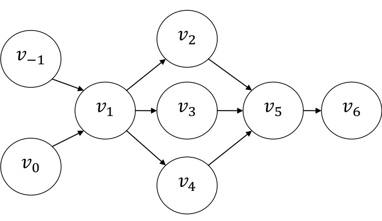
effectively follow variables through a program, a “computational graph” is often used to give
Table 2-1: Evaluation Trace for Equation (4)
= = 2.000
= = 1.000
= = 2.000/1.000 = 2.000
= = = 3.762
= = = 0.9093
= = = 7.389
= =
= 0.5600
= = = 5.120
Figure 2.1: Computation Graph of Table 2-1
2.1.1 Forward Mode
Many AD packages feature two ways to follow the evaluation trace of the program.
The first and most basic way that an AD package can operate is by calculating the derivatives
of the inputs and following the evaluation trace to the outputs, calculating the derivatives of
each intermediate along the way. In the example presented earlier, in order to calculate
derivatives of y with respect to , each intermediate variable must be differentiated with
respect to and evaluated for the desired values of and . This will create new
intermediate derivative variables ( ) that will be associated with each
corresponding intermediate variable. Starting with the first line in Table 2-1 it is easy to see
that and . Moving to gives the following:
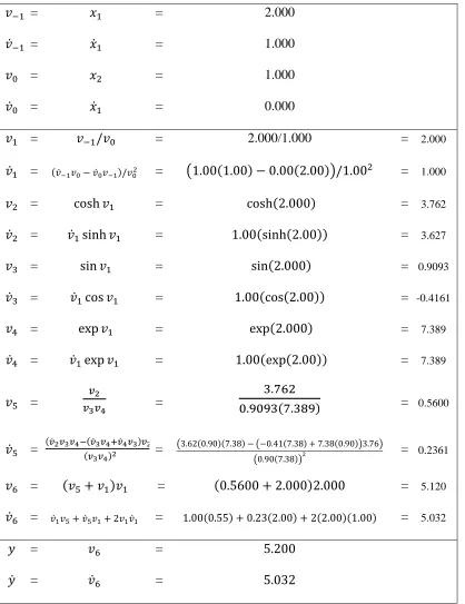
Table 2-2 gives the full evaluation trace for the forward calculation of derivatives. If
derivatives with respect to are desired, the process can be repeated but instead
and . For problems with multiple outputs, the forward mode can be
used to obtain the derivatives of each desired output variable with respect to a single input
variable in one run. This makes the forward mode more desirable to use when the number of
Table 2-2: Forward mode evaluation trace
= = 2.000
= = 1.000
= = 1.000
= = 0.000
= = 2.000/1.000 = 2.000
= = = 1.000
= = = 3.762
= = = 3.627
= = = 0.9093
= = = -0.4161
= = = 7.389
= = = 7.389
=
=
= 0.5600
=
=
= 0.2361
= = = 5.120
= = = 5.032
= =
2.1.2 Reverse Mode
In addition to the forward mode, some AD packages (including OpenAD) feature a
reverse or adjoint mode. Instead of selecting an independent variable and calculating the
derivatives of every intermediate variable with respect to that variable, a dependent variable
is chosen and the derivatives of that variable with respect to each intermediate variable are
calculated [1]. In order to perform an evaluation trace in the reverse mode, new adjoint
variables will be defined. Let
(in a strict sense, actually is defined to be
where
is a new independent variable added to the right-hand side of the equation defining [1]).
The evaluation trace starts from the final steps of the normal evaluation trace and works
backwards, hence reverse mode. The desired dependent adjoint variable will be set to 1.000,
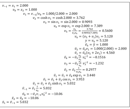
which for this case of a single output means that Table 2-3 gives the normal
evaluation trace followed by the evaluation trace for a reverse mode derivative calculation.
Note that each line in the reverse mode calculation is lined up with the corresponding line of
the model calculation above. The application of the chain rule in reverse mode can be
confusing, so as an example, consider tracing backwards through the model calculation to the
line . Here, depends on and . The adjoint variables corresponding
to this line are and
. Noting that
and
evaluating the current expression for to get the other required derivatives gives
the next step, , and repeat. For variables that appear multiple times in the trace
(such as ), the previously calculated adjoint values are accumulated into the new
calculation (as is shown in the lines and ).
The value
obtained in the reverse mode trace agrees with what was
obtained in the forward trace shown in Table 2-2. Also note that
was calculated in the
reverse mode trace with only a single extra calculation. This makes the reverse mode useful
for models where the number of inputs is greater than the number of outputs. However, the
reverse mode transformation can be difficult to implement due to the fact that the evaluation
trace must be reversible which can be an issue for some model codes.
2.1.3 Active Variables
The concept of an ‘active variable’ is important to AD. An ‘active variable’ is any
variable in the model that comes into contact via assignment to the dependent/independent
variables. For example, in a program that computes from in the following fashion:
and
is the value desired by AD calculation, the active variables are and . The
parameters and are viewed as ‘passive variables’ as they are not assigned values that
variables in OpenAD and Rapsodia require type changes from real, double precision, etc. to
a custom defined active type in order to operate.
2.2
OpenAD
OpenAD uses association by address [5], that is an active type, as the means of
augmenting the original program data to hold the derivative information. The usual activity
analysis would ordinarily trigger the re-declaration of only a subset of common block
variables. Because the access of the common block via the array enforces a uniform type for
all common block variables to maintain proper alignment, all common block variables had to
be activated. Furthermore, because the equivalence construct applied syntactically only to
the first common block variable, the implicit equivalence of all other variables cannot be
automatically deduced and required a change of the analysis logic for OpenAD to maintain
alignment by conservatively overestimating the active variable set. Superficially this may
seem a drawback of the association by address. The association by name [10], used in other
AD source transformation tools will not fare better though. Shortening the corresponding
loop for the name-associated and equivalenced derivative-carrying array is difficult for
interspersed passive data and therefore one will resort to the same alignment requirement.
2.3
Rapsodia
Rapsodia is based on operator overloading for the forward propagation of univariate
Table 2-3: Reverse mode evaluation trace
operators that are hand-coded, operate on Taylor coefficient arrays with variable length in
loops with variable bounds to accommodate the derivative orders and numbers of directions
needed by the application. In contrast, Rapsodia generates on demand a library of
overloaded operators for a specific number of directions and a specific order. Thus, at
compile time, the loops are already represented in (partially) unrolled code along with a fixed
(partially flat) data structure that provides more freedom for compiler optimization. Because
of the overall assumption that r, the reduced input dimension, is much smaller than m the
higher order derivative computation in forward mode is feasible and appropriate.
Because overloaded operators are triggered by using a special (active) type for which
they are declared it now appears as a nice confluence of features that OpenAD for the
gradient computation already does the data augmentation via association by address, i.e. via
an active type, and therefore the assumption could be made that one merely has to change the
OpenAD active type to a Rapsodia active type to use the operator overloading library.
2.4
Efficient Subspace Method
Subspace methods are based on mathematical ideas in linear algebra. The key
components are the vector spaces that exist in matrix representations of the inputs and
outputs of a model in question. The goal of using subspace methods in relation to the method
presented here is to determine a low rank approximation of the model using information
gathered from the first order sensitivity (Jacobian) matrix. The effective rank that is desired
independent piece of information in the input/output stream [8]. An active DOF denotes a
DOF that is transferred from a higher to a lower resolution model, and an inactive DOF
denotes one that is thrown out [8].
A very important tool used in subspace methods is the matrix decomposition.
Examples of common matrix decompositions are the QR factorization and singular value
decomposition (SVD). For an Jacobian matrix with rank ,the SVD
is given by:
(5)
where and are full column rank orthonormal matrices that constitute
orthonormal bases for the vector spaces and , respectively. is a nonsingular
diagonal matrix whose elements correspond to the singular values (usually organized from
largest to smallest) of .
The SVD is a so called ‘rank revealing’ decomposition because the number of
non-zero singular values correspond to the numerical rank of the original matrix. In practice, all
singular values will be non-zero, but the SVD still allows for the ‘effective’ rank to be
determined. Only the largest singular values will count towards the effective rank. The
cutoff criterion that determines which singular values count towards the effective rank can
By determining an effective rank of a matrix which is lower than , a low
rank approximation can be constructed. After determining the effective rank by inspection of
the SVD or by using the rank finding algorithm that will be introduced in the next section, a
number of vectors corresponding to the size of the active subspace can be used in
constructing a low rank approximation.
2.5
General Methodology
To start, a simple example of constructing a low rank approximation to a matrix
operator will be considered. Let the matrix in question in be . The elements of
are not known, but the ability to perform matrix vector products with and is available.
The steps involved in determining a low rank approximation of are as follows:
1. Use k random Gaussian input vectors to compute k matrix vector products:
2. Perform a QR decomposition on the responses:
3. Determine the effective rank
r
using the Rank Finding Algorithm (RFA):a. Choose a small integer k
b. Choose a sequence of k random Gaussian vectors
wi ik14. If rk, continue. Otherwise, add more matrix vector products in step 1 and repeat
steps 2 and 3
5. Calculate pi ATqi for all i
6. Using the pi and qi vectors, a low rank approximation of the form T A USV can
be calculated as shown in the appendix of [9].
It has been shown in other works [12] that the effective rank
r
can be determined with atleast probability when Q satisfies the following criterion:
(6)
where is the user specified error allowance. In real applications, these ideas can be applied
by replacing the matrix operator with a computational model. Let the computational model
of interest be described by a vector valued function:
where and . The goal of this methodology is to compute the entire set of
derivatives for a given order by reducing the dimensions of the problem and thus reducing
single-reference point as follows (without loss of generality, assume that and
in order to simplify the representation):
(7)
where can be any kind of scalar functions. The outer summation over the variable k
goes from 1 to infinity. Each term represents one order of variation, e.g. k 1 represents
the first order term; k 2, the second order terms. For the case of , the th
k term
reduces to the th
k term in a multi-variable Taylor series expansion. The inside summation
for the th
k term consists of k single valued functions that are multiplying each other.
The arguments for the functions are scalar quantities representing the inner products
between the vector and n vectors
which span the parameters space. The
superscript ( )k implies that a different basis is used for each of the k-terms, i.e. one basis is
used for the first-order term, another for the second-order term and so on.
Any input parameter variations that are orthogonal to the range formed by the
collection of the vectors will not produce changes in the output response, i.e. the
value of the derivative of the function will not change. If the vectors span a subspace
from n to r. The mathematical range can be determined by using only the first-order
derivatives.
Differentiating Eq. (7) with respect to x gives:
(8)
where
l l
k T k
l j x j
is the derivative of the term
l
k T
l j x
. Eq. (3) can be reinterpreted
to show that the gradient of the function is a linear combination of the { }
l
k j
vectors:
(9) where (10)
After determining the effective rank, it can be seen that the function only depends on r
effective dimensions and can be reduced to simplify the calculation. The reduced model only
requires the use of the subspace that represents the range of B, of which there are infinite possible bases.
This concept will now be expanded to a multi-response model. The qth response of
the model and its derivative are given by:
(11)
(12)
The active subspace of the overall model must contain the contributions of each individual
response. The matrix B will contain the vectors for all orders and responses. To determine a low rank approximation, a pseudo response will be defined as a
(13)
where q are randomly selected scalar factors. The gradient of the pseudo response is:
(14)
Calculating derivatives of the pseudo response as opposed to each individual response
provides the necessary derivative information while saving considerable computational time
CHAPTER 3
Implementation
3.1
Implementation on a General FORTAN Code
The computational model that is executed in the computer code of interest will be
assumed to be of the following form:
(15)
where y is an m1 vector whose components correspond to the m outputs of interest, x is an
1
n vector whose components correspond to the n inputs of interest, and corresponds to
the unknown operator acting on the inputs to produce output. No previous information of
is needed; only the ability to obtain y from x is necessary for this method to work. The next
step is to define the pseudo response y:
(16)
where yi are the individual components of the response vector y. This will be done with an
invasive definition in the computer code, preferably in the highest level routine. Once the
pseudo response has been defined, the reverse mode of OpenAD will be utilized to obtain
form of the code is created to calculate the n1 vector
, the active subspace of the model
will be found by generating a set of derivative vectors, which span the union of all
single-responses active subspace. The code will be run using a random set of inputs, .
The responses will then be collected into the columns of an n k matrix G:
(17)
Now, the effective rank of G will be found via the Rank Finding Algorithm (RFA).
(18)
where the sub-matrix contains only the first r columns of . The rank is selected
in the RFA to satisfy a user defined error metric such that
(19)
where is the norm. The columns of the matrix will be used to define the pseudo
inputs that will be coded into a version of the code that will be used with Rapsodia to
calculate derivatives of the output responses with respect to the pseudo inputs of a desired
order. The pseudo inputs are defined as:
In order to satisfy the logical order of derivative calculation by means of the chain rule of
differentiation dy dy dx
dx dx dx
, x will be defined in the code in terms of x and the columns of
:
(21)
This line is what must be inserted into the code, preferably in the top level routine. Now
Rapsodia will be used to create an executable version of the code that calculates
1 ( ) ( ) ( ) 1... n O o o n d y dx dx
where O is the desired derivative order and o1 ... on O. For first order calculations, the
full derivatives can be recovered utilizing the following relation that comes from the chain
rule of differentiation:
(22)
The following matrix operation can also be used: where is the matrix of derivatives
with respect to the pseudo variables. From Eq.(20), it can easily be determined that
. For orders greater than 1, the mixed derivatives play a part in the reconstruction. The
following equation shows how the second order derivatives are reconstructed on an element
(23)
The following matrix operation can also be used: where is the matrix of
second order derivatives of response i with respect to the pseudo variables. For example, the
second derivative of output i = 1 with respect to input j = 1 in a problem with an effective
rank of r = 2 would be recovered by
2 2 2 2
2 2
1 1 1
11 11 12 12
2 2 2
1 1 1 2 2
1 2
d y d y d y d y
q q q q
dx dx dx dx dx . Mixed
derivatives would be recovered by:
2 2
,
i i
jk gl k l
j g k l
d y d y q q
dx dx
dx dx (20)In the same case as before (r = 2),
2 2 2 2
1 1 1 1
11 12 11 22 12 21 12 22
2 2
1 1 1 1 2 2
d y d y d y d y
q q q q q q q q
dx dx dx dx dx dx .
It can be inferred that for derivatives of order O, the non mixed derivatives can be recovered
using the following expression:
( ) ( )
( )
, ,... ...
O O
i i
jk jl jz
O
k l o
j k l z
d y d y
q q q
where the total number of different indices k, l,..z is O and each index runs from 0 to n . The
mixed derivatives are:
( ) ( )
, ...
...
... ...
O O
i i
jk gz
k l o
j g k z
d y d y
q q
dx dx
dx dx (22)The algorithm detailed in this section can be summarized as follows:
1. Define the pseudo responses in the top level routine (Eq. 11)
2. Compile an executable using OpenAD to compute dy
dx
3. Run the dy
dx calculation k times and assemble the output into a matrix G (Eq. [12])
4. Determine the effective rank r using the RFA
5. Calculate a QR decomposition of G and keep the first r columns of Q in Qr (Eq.
[15])
6. Define the inputs in terms of the pseudo inputs and Qr in the top level routine (Eq. [17])
7. Reconstruct the full derivatives (Eq.[18])
1. Calcuate the SVD of G: T
G USV
2. Set the smallest singular value to 0 and keep the remaining r singular values: p 0
3. Calculate an approximation of G: GUS Vr T
Repeat steps 2 and 3 until || ||
|| ||
G G
CHAPTER 4
Examples and Test Cases
4.1
Two-minute AD Examples
To quickly introduce the two AD tools used in this method, ‘Two-minute’ examples
will be shown to illustrate the basics of how to use each tool on a subroutine containing an
easily differentiated function. The examples follow the basic style given in the examples
used in the OpenAD/F Manual [10] and Rapsodia Manual [5]. The manuals should be
consulted for a more in depth presentation of the inner workings of each tool.
4.1.1 OpenAD/F Example
A simple subroutine will be used to illustrate the calculation of derivatives using
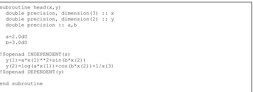
OpenAD. Figure 4.1 shows the subroutine that will be used in this example. The function
that the subroutine models consists of two outputs (y) and three inputs (x). The parameters
a, and b are simply scalar factors used in the calculation. The only additions to this code that
are required by OpenAD are the tags identifying the independent (!$openad INDEPENDENT(x))
and dependent variables (!$openad DEPENDENT(y)). The goal is to calculate the derivatives of
each output with respect to each input. A main program called driver will be used with
subroutine head in order to extract the derivatives. Figure 4.2 shows the main program
Figure 4.1: Simple subroutine for ‘Two-minute’ forward OpenAD example
program driver use OAD_active implicit none external head
type(active) :: x(3), y(2) x(1)%v=1.0D0 x(2)%v=2.0D0 x(3)%v=3.0D0 x(1)%d=1.0D0 x(2)%d=0.0D0 x(3)%d=0.0D0 call head(x,y)
print *, 'driver running for x =',x%v
print *, ' yields y =',y%v,' dy/dx =',y%d
x(1)%d=0.0D0 x(2)%d=1.0D0 x(3)%d=0.0D0 call head(x,y)
print *, 'driver running for x =',x%v
print *, ' yields y =',y%v,' dy/dx =',y%d
x(1)%d=0.0D0 x(2)%d=0.0D0 x(3)%d=1.0D0 call head(x,y)
print *, 'driver running for x =',x%v
print *, ' yields y =',y%v,' dy/dx =',y%d
end program driver subroutine head(x,y)
double precision, dimension(3) :: x double precision, dimension(2) :: y double precision :: a,b
The active type declaration shown in line 5 must be used in this top level routine for
the active variables. The active type will give each active variable two parts, a normal value
(indicated by %v) and a derivative part (%d). Lines 6, 7 and 8 initialized the value parts of
x. Before the subroutine is called, one input will be chosen for derivative calculation. This
variable’s derivative part will be ‘seeded’ with a value of 1 while all others are assigned 0.
For the first call of head, this can be viewed as starting with
and
as is shown in Table 2-2: Forward mode evaluation trace. For subsequent calls of head, the
seed will change to the other inputs. The basic call to invoke the OpenAD tool for a forward
transformation is openad –m f [file name] which will create a new transformed
file. After transforming and compiling all the necessary files for the example given above,
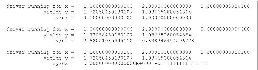
the following output given in Figure 4.3: Output for the ‘Two-minute’ forward OpenAD
example is returned.
The forward mode allows for the calculation of derivatives of each output with
respect to one input at a time. As a quick check, the first set of derivative values given are
and
. The derivatives evaluated for can easily be found analytically:
and .
An example that requires more precision is
When the analytically derived
expression is evaluated in Matlab for , the first 14 digits match exactly.
The Makefile shown in Figure 4.4: Makefile contents for compiling and linking
Figure 4.3: Output for the ‘Two-minute’ forward OpenAD example
Figure 4.4: Makefile contents for compiling and linking the ‘Two-minute’ forward OpenAD example
ifndef F90C F90C=ifort endif
RTSUPP=w2f__types OAD_active
driver: $(addsuffix .o, $(RTSUPP)) driver.o head.prepped.pre.xb.x2w.w2f.post.o ${F90C} -o $@ $^
head.prepped.pre.xb.x2w.w2f.post.f90 $(addsuffix .f90, $(RTSUPP)) : toolChain toolChain : head.prepped.f90
openad -c -m f $< %.o : %.f90
${F90C} -o $@ -c $< clean:
rm -f ad_template* OAD_* w2f__* iaddr*
rm -f head.prepped.pre* *.B *.xaif *.o *.mod driver driverE *~ .PHONY: clean toolChain
# the following include has explicit rules that could replace the openad script include MakeExplRules.inc
driver running for x = 1.00000000000000 2.00000000000000 3.00000000000000 yields y = 1.72058450180107 1.98665080054364
dy/dx = 4.00000000000000 1.00000000000000
driver running for x = 1.00000000000000 2.00000000000000 3.00000000000000 yields y = 1.72058450180107 1.98665080054364
dy/dx = 2.88051085995110 0.838246494596778
driver running for x = 1.00000000000000 2.00000000000000 3.00000000000000 yields y = 1.72058450180107 1.98665080054364
compiling all the necessary files for the example shown above. After running the
Makefile, an executable named ‘driver’ is created. The Fortran compiler used is ifort.
To operate in the reverse mode, the prepped subroutine does not require changes.
The main program driver will require some slight modifications. Figure 4.5 contains the
reverse mode driver.
The main difference between the forward and reverse mode main programs is that the
seeding is done with the outputs in the reverse mode. The derivatives of one output with
respect to all inputs are calculated at once in the reverse mode. The reverse mode flag must
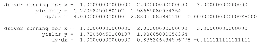
be used when executing the OpenAD tool (openad –m rj [file name]). Figure 4.6
gives the output for the reverse mode example.
The outputs exactly match those given by the forward mode. When using OpenAD
on more complex codes, the same basic methods presented in these examples are used.
4.1.2 Rapsodia Example
Rapsodia will now be used to calculate first, second, and third order derivatives of the
function in the subroutine from the previous example. The subroutine itself does not require
many changes. Rapsodia does not require the tags that OpenAD used, but the active
variables must be changed to the Rapsodia active type in both the subroutine and main
Figure 4.5: Example reverse mode main program
Figure 4.6: Reverse mode example output
subroutine head(x,y) INCLUDE 'RAinclude.i90' TYPE(RARealD) :: x(3),y(2) double precision :: a,b
a=2.0d0 b=3.0d0
y(1)=a*x(1)**2+sin(b*x(2))
y(2)=log(a*x(1))+cos(b*x(2))+1/x(3)
driver running for x = 1.00000000000000 2.00000000000000 3.00000000000000 yields y = 1.72058450180107 1.98665080054364
dy/dx = 4.00000000000000 2.88051085995110 0.000000000000000E+000
driver running for x = 1.00000000000000 2.00000000000000 3.00000000000000 yields y = 1.72058450180107 1.98665080054364
dy/dx = 1.00000000000000 0.838246494596778 -0.111111111111111 program driver
use OAD_active use OAD_rev implicit none external head
type(active) :: x(3), y(2) x(1)%v=1.0D0 x(2)%v=2.0D0 x(3)%v=3.0D0 y(1)%d=1.0D0 y(2)%d=0.0D0 our_rev_mode%tape=.TRUE. call head(x,y)
print *, 'driver running for x =',x%v
print *, ' yields y =',y%v,' dy/dx =',x%d
y(1)%d=0.0D0 y(2)%d=1.0D0
our_rev_mode%tape=.TRUE. call head(x,y)
print *, 'driver running for x =',x%v
print *, ' yields y =',y%v,' dy/dx =',x%d
The main program logic that is required for running Rapsodia on this subroutine is
more involved than OpenAD, but it can mostly be reused easily for any general subroutine or
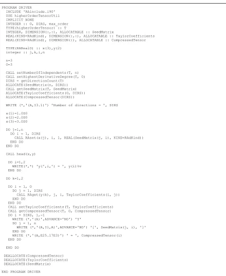
program. Figure 4.8 gives the complete main program that was used to run the Rapsodia
example.
Lines 2-9 contain the Rapsodia specific variable declarations. These variables are
initialized in lines 17-23 by calling Rapsodia specific routines that are generated and must be
compiled with the program. The desired independent variables are set in the loops of lines
31-35 with the call to RAset. The derivatives are extracted and output in lines 45-58, which
are looped over for each output. The call to RAget sets the dependent variables. A
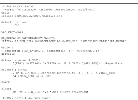
Makefile is shown in Figure 4.9 which contains the instructions for generating the
necessary files from the Rapsodia library and linking them to the subroutine and main
program. The line ${RAPSODIAROOT}/Generator/generate.py -d 3 -o 1 -f $(GEN_DIR) must
be set with the appropriate number of directions (d) and derivative order (o). For first order
derivatives of this example, the values are 3 and 1, respectively. Again, an executable named
‘driver’ is created to run the program.
Figure 4.10 through Figure 4.12 contain the results for first through third order
derivatives. The only changes required to obtain a different order of derivatives are
rebuilding the program after changing the order number in the main program and Makefile
and changing the number of directions in the Makefile. The results are printed with the
Figure 4.8: Main program for the ‘Two-minute’ Rapsodia example
PROGRAM DRIVER
INCLUDE 'RAinclude.i90' USE higherOrderTensorUtil IMPLICIT NONE
INTEGER :: O, DIRS, max_order TYPE(higherOrderTensor) :: T
INTEGER, DIMENSION(:,:), ALLOCATABLE :: SeedMatrix
REAL(KIND=RAdKind), DIMENSION(:,:), ALLOCATABLE :: TaylorCoefficients REAL(KIND=RAdKind), DIMENSION(:), ALLOCATABLE :: CompressedTensor TYPE(RARealD) :: x(3),y(2)
integer :: j,k,i,n n=3
O=3
CALL setNumberOfIndependents(T, n) CALL setHighestDerivativeDegree(T, O) DIRS = getDirectionCount(T)
ALLOCATE(SeedMatrix(n, DIRS)) CALL getSeedMatrix(T, SeedMatrix) ALLOCATE(TaylorCoefficients(O, DIRS)) ALLOCATE(CompressedTensor(DIRS))
WRITE (*,'(A,I3.1)') 'Number of directions = ', DIRS x(1)=1.0D0
x(2)=2.0D0 x(3)=3.0D0 DO j=1,n
DO i = 1, DIRS
CALL RAset(x(j), i, 1, REAL(SeedMatrix(j, i), KIND=RAdKind)) END DO
END DO
CALL head(x,y) DO i=1,2
WRITE(*,*) 'y(',i,') = ', y(i)%v END DO
DO k=1,2 DO i = 1, O DO j = 1, DIRS
CALL RAget(y(k), j, i, TaylorCoefficients(i, j)) END DO
END DO
CALL setTaylorCoefficients(T, TaylorCoefficients) CALL getCompressedTensor(T, O, CompressedTensor) DO i = DIRS, 1,-1
WRITE (*,'(A)',ADVANCE='NO') 'Y' DO j = 1, n
WRITE (*,'(A,I1,A)',ADVANCE='NO') '[', SeedMatrix(j, i), ']' END DO
WRITE (*,'(A,E25.17E3)') ' = ', CompressedTensor(i) END DO END DO DEALLOCATE(CompressedTensor) DEALLOCATE(TaylorCoefficients) DEALLOCATE(SeedMatrix)
Figure 4.9: Makefile contents for compiling and linking the ‘Two-minute’ Rapsodia example (first order)
ifndef RAPSODIAROOT
$(error "environment variable RAPSODIAROOT undefined") endif
include ${RAPSODIAROOT}/Makefile.inc
default: driver ./$^
GEN_DIR=RALib
RA_EXTRAS=${RAPSODIAROOT}/hotF90
IPATH+=-I$(GEN_DIR) $(MODSEARCHFLAG)$(GEN_DIR) $(MODSEARCHFLAG)$(RA_EXTRAS)
OBJS= \
$(addprefix $(RA_EXTRAS)/, $(addsuffix .o,$(HOTF90NAMES))) \ driver.o
driver: sources $(OBJS)
$(F90C) $(FFLAGS) $(IPATH) -o $@ $(OBJS) $(GEN_DIR)/libRapsodia.a
sources : FORCE
${RAPSODIAROOT}/Generator/generate.py -d 3 -o 1 -f $(GEN_DIR) cd $(GEN_DIR) && $(MAKE)
FORCE:
clean:
rm -rf $(GEN_DIR) *.o *.mod driver driver.out
derivative that is first order in and second order in .
Like the OpenAD example, these same basic steps are used in the examples and test
cases that follow.
4.2
Matrix-Vector Product Example
This example will now implement the reduction method on a pre-constructed low
rank matrix operator. To start, consider a random matrix . The matrix will be
modified so that it is rank deficient by zeroing singular values. To visualize a rank
deficient matrix, consider a 2D plane in a 3D space. Consider different vectors that live
inside the plane. Since the plane is 2 dimensional, any vector inside it can be expressed as a
linear combination of two vectors only (any two independent vectors that live inside the
plane). In this case the matrix would have rank equal to 2 only and not . In order to
reduce this problem, one needs to find any two vectors that live in that plane. The simplest
way to do this is to run the reverse mode twice, once for
and once for
.
However, this does not guarantee that
and
are linearly independent vectors.
To get around that, a new ‘pseudo’ response will be defined. Let .
The new variables are simply weighted (the weights can be picked randomly) sums of the
Figure 4.10: Rapsodia example first order results
Figure 4.11: Rapsodia example second order results Number of directions = 6
y( 1 ) = 1.7205845018010741 y( 2 ) = 1.9866508005436445
Y[2][0][0] = 0.40000000000000000E+001 Y[1][1][0] = 0.00000000000000000E+000 Y[1][0][1] = 0.00000000000000000E+000 Y[0][2][0] = 0.25147394837903327E+001 Y[0][1][1] = 0.00000000000000000E+000 Y[0][0][2] = 0.00000000000000000E+000
Y[2][0][0] = -0.10000000000000000E+001 Y[1][1][0] = 0.00000000000000000E+000 Y[1][0][1] = 0.00000000000000000E+000 Y[0][2][0] = -0.86415325798532940E+001 Y[0][1][1] = 0.00000000000000000E+000 Y[0][0][2] = 0.74074074074074070E-001 Number of directions = 3
y( 1 ) = 1.7205845018010741 y( 2 ) = 1.9866508005436445
Y[1][0][0] = 0.40000000000000000E+001 Y[0][1][0] = 0.28805108599510980E+001 Y[0][0][1] = 0.00000000000000000E+000
Figure 4.12: Rapsodia example third order results Number of directions = 10
y( 1 ) = 1.7205845018010741 y( 2 ) = 1.9866508005436445
Y[3][0][0] = 0.00000000000000000E+000 Y[2][1][0] = 0.46678715293069217E-006 Y[2][0][1] = 0.00000000000000000E+000 Y[1][2][0] = 0.37342972254439388E-005 Y[1][1][1] = 0.46678715304171448E-006 Y[1][0][2] = 0.00000000000000000E+000 Y[0][3][0] = -0.25924587937029660E+002 Y[0][2][1] = 0.37342972269982511E-005 Y[0][1][2] = 0.46678715293069217E-006 Y[0][0][3] = 0.00000000000000000E+000
(24)
Equation (24) is simply a random sum of the rows of the matrix . If the weights are
selected randomly, there is a high probability that
and
will be independent.
This approach can be generalized for a matrix with rank . Let the model be
described by . For now assume that the matrix is random and constructed to be rank
deficient with known rank . A pseudo response will be constructed as shown
above. Using reverse mode OpenAD, sets of derivatives of the pseudo response will be
taken. Figure 4.13 shows the code for a matrix vector product with the pseudo response
definition.
The collection of derivatives that are obtained,
, are now
used to define pseudo inputs of the form . In order to keep the logical progression of
variables for the OpenAD evaluation trace in the code, will be defined in terms of :
. Forward mode OpenAD will then be used to obtain
Figure
4.14 shows the code for a matrix vector product with the pseudo input definition.
The full derivatives
(which in this case are the same as the matrix) can be recovered by
multiplying the reverse results by the forward results:
Figure 4.13: Matrix-vector product code with pseudo response definition
Figure 4.14: Matrix-vector product code with pseudo input definition !$openad INDEPENDENT(x_pseudo)
do j=1,r do i=1,n
x(i)=x(i)+x_pseudo(j)*J_pseudo(i,j) end do
end do do i=1,m do j=1,n
y(i)=y(i)+A(i,j)*x(j) end do
end do
!$openad DEPENDENT(y) !$openad INDEPENDENT(x)
do i=1,m do j=1,n
y(i)=y(i)+A(i,j)*x(j) end do
end do
do j=1,r do i=1,m
y_pseudo(j)=y_pseudo(j)+y(i)*gamma(i,j) end do
end do
In realistic problems, the rank will not be absolute, i.e. all singular values will be
non-zero, but the magnitudes of the singular values will be distributed such that an effective
rank can be determined. Another random rank deficient matrix will be used to demonstrate
how the rank finding algorithm works. A random matrix with the singular value
distribution shown in Figure 4.15 will be considered for this example.
The singular value distribution shows that of the 500 singular values, only about 60
actually contribute significantly. A safe estimate of the effective rank would be 100.
Obtaining the unreduced derivatives will yield the original matrix. By doing an SVD on this
output and taking the first 50 columns of the matrix, , pseudo inputs can be defined as
shown above. The output of the derivatives of the responses with respect to the
pseudo inputs will be multiplied by to obtain the reduced approximation of Using an
effective rank of 100 yields a maximum matrix element relative error of 0.130%.
To advance the demonstration of this method further towards actual engineering
codes, the next examples will demonstrate when the rank must be determined by means of
4.3
Scalar-valued Model Example
First, a scalar valued function will be considered. The model that will be considered
is:
(25)
where x, a, b, c, and d are n1 vectors, making y a scalar valued function. A simple
subroutine named 'head' was written to calculate this model along with a simple main
program called a 'driver' that calls the subroutine and is used to extract the derivatives. In
order to prepare the code for use with OpenAD, tags must be inserted to identify the
independent and dependent variables (typically formal parameters of ‘head’) to the code
analysis. Within ‘driver’ the corresponding inputs and outputs, passed as actual parameters
to ‘head’, have to be declared with the OpenAD active type to carry the derivative values.
After the code is prepared in this fashion for use with OpenAD, it generates a transformed
version of 'head', which then is compiled together with ‘driver’ and calculates the first order
derivatives of y with respect to the vector x.
A Python script was written to execute the subspace identification algorithm with the
compiled executable code. The script takes a guess k for the effective rank and runs the code
for k random input vectors x. Within the Python script, the responses are collected into a
matrix of dimension n k . is then QR factorized and the first r columns of are used
evaluate the error. If the error criterion is met, the first r columns of are written to a file to
be used as input for the higher-order derivative computation with Rapsodia. Figure 4.16
shows the Python script used with this model. For the model above with n = 50 and random
input vectors with 8 digits of precision for a, b, c, and d with an error criterion of 6
10
,
the effective rank was found to be r = 3.
A process similar to the one for OpenAD is used to prepare the program for use with
Rapsodia. The active variables are identified via a similar manual type change in the 'driver'
and the source transformation capabilities of OpenAD can be used to perform the type
change in the ‘head’ subroutine. Because of the additional steps to determine the
propagation directions and compute the derivative tensors, the logic in the 'driver' has
additional steps for Rapsodia, but they follow a simple recipe and can be transferred between
such driver programs with relative ease. For efficiency, the number of directions that the
derivatives are calculated for along with the desired derivative order must be provided to the
library generator implemented by Rapsodia. Once the library is generated, the type-changed
‘head’, the ‘driver’, and the library can be compiled and linked. For first order calculations,
the number of directions is simply the number of input variables for which derivatives are
calculated. Once the derivatives
are calculated, the full derivatives can be reconstructed
by multiplying the Rapsodia results by the matrix used as input. Using an effective rank
of , the reconstructed derivatives were found to have relative errors on the order of
13
Figure 4.16: Python script used for the scalar-valued model example while (z>e):
while (i<k):
#run the forward driver
status,output=commands.getstatusoutput('./driver ' + str(n) ) print status
#input to G from output of driver G[:,i]=numpy.genfromtxt('der_out.txt') j=0 while (j<n): In[j,5]=10*random.random() j=j+1 numpy.savetxt('Rinput.in.txt',In) i=i+1
#calculate QR of G Q,R=linalg.qr(G) Qr=Q[:,0:k]
#generate additional samples for error testing Gadd=numpy.zeros((n,k)) p=0 while (p<k): j=0 while (j<n): In[j,5]=10*random.random() j=j+1 numpy.savetxt('Rinput.in.txt',In) #run the forward driver
status,output=commands.getstatusoutput('./driver ' + str(n) ) print status
#input to Gadd from output of driver Gadd[:,p]=numpy.genfromtxt('der_out.txt') p=p+1
z=linalg.norm( dot( numpy.eye(n)-dot(Qr,Qr.T),Gadd) ) print z k=k+1 Gnew=numpy.zeros((n,k)) Gnew[:,0:k-1]=G numpy.savetxt('Gnew',Gnew) G=numpy.zeros((n,k)) G=Gnew numpy.savetxt('G',G)
Using Rapsodia to calculate second order derivatives simply involves changing the
derivative order (o = 2) and the number of directions (d = 6) to regenerate the library and
recompiling the code. The output can then be constructed into a matrix of size
r r
andthe full derivatives can be recovered by: which results in an n n symmetric matrix.
When the second order derivatives are calculated for the example above, there are only 6
directions required for an effective rank of 3 as opposed to 1275 directions for the full
problem. The relative errors of the reduced derivatives are on the order of 12
10 .
Third order derivatives were also calculated using this example. The unreduced
problem would require 22,100 directions while the reduced problem only requires 10.
Relative errors were much higher for this case but still at a reasonable order of 6
10 . The
relative errors for each derivative order are summarized in Table 4-1. The maximum
unreduced relative error is the maximum relative error between the unreduced Rapsodia
calculations and analytical results. The average unreduced relative errors are on the order of
. Note that for the third order calculations, not all values for the unreduced case were
calculated due to the difficulty of obtaining all values at once. The full codes for this
Table 4-1: Results for the scalar-valued model example
Derivative Order
Unreduced Directions
Reduced Directions
Reduced Relative Error
Maximum Unreduced Relative Error
1 50 3 10-13 1.49%
2 1275 6 10-12 4.21%
4.4
Vector-valued Model Example
It is important to note here that in practice the derivatives are employed to construct a
surrogate model that approximates the original function. Therefore, it is much more
instructive to talk about the accuracy of the surrogate model employed rather than the
accuracy of each derivative. This is illustrated in the MATWS test case by using an
engineering model.
Problems with multiple outputs require a slightly different approach when
determining the subspace. The following example will be considered:
(26)
In the OpenAD version of the subroutine, the responses will be combined into a pseudo
response defined by the following:
(27)
where are randomly generated factors that are unique for each execution of the code. The
derivatives that OpenAD will calculate are
, which is an n1 vector. Following the same