University of Warwick institutional repository: http://go.warwick.ac.uk/wrap
This paper is made available online in accordance with
publisher policies. Please scroll down to view the document
itself. Please refer to the repository record for this item and our
policy information available from the repository home page for
further information.
To see the final version of this paper please visit the publisher’s website.
Access to the published version may require a subscription.
Author(s): Yinyin Yuan and Chang-Tsun Li;
Article Title: Inferring Causal Relations from Multivariate Time Series:
A Fast Method for Large-Scale Gene Expression Data
Year of publication: 2009
Link to published article:
http://dx.doi.org/10.1109/BIBE.2009.8
Publisher statement: ("(c) 2009 IEEE. Personal use of this material is
permitted. Permission from IEEE must be obtained for all other users,
including reprinting/ republishing this material for advertising or
Inferring Causal Relations from Multivariate Time
Series: A Fast Method for Large-Scale Gene
Expression Data
Yinyin Yuan and Chang-Tsun Li
Department of Computer Science
University of Warwick, Coventry, United Kingdom Email: yina,[email protected]
Abstract—Various multivariate time series analysis techniques have been developed with the aim of inferring causal relations between time series. Previously, these techniques have proved their effectiveness on economic and neurophysiological data, which normally consist of hundreds of samples. However, in their applications to gene regulatory inference, the small sample size of gene expression time series poses an obstacle. In this paper, we describe some of the most commonly used multivariate inference techniques and show the potential challenge related to gene expression analysis. In response, we propose a directed partial correlation (DPC) algorithm as an efficient and effective solution to causal/regulatory relations inference on small sample gene expression data. Comparative evaluations on the existing techniques and the proposed method are presented. To draw reliable conclusions, a comprehensive benchmarking on data sets of various setups is essential. Three experiments are designed to assess these methods in a coherent manner. Detailed analysis of experimental results not only reveals good accuracy of the proposed DPC method in large-scale prediction, but also gives much insight into all methods under evaluation.
I. INTRODUCTION
One major step in recent genomic research is the advance of high-throughput microarray technique, which allows ex-pression levels of all genes in the genome to be measured at particular time points. The resulting gene expression dynamics are important, since they directly reveal the active components within the cell over time, indicating gene regulatory relation-ships on the transcriptional level. However, they also pose a dimensionality problem in the subsequent data analysis, with the number of genes far exceeding the number of samples/time points [1]. The situation is quite the opposite to classical time series analysis, thus objective technique is needed for learning gene regulatory relationships from these data. Also, large number of genes/variables poses a challenge to interaction inference in a directed form, since there are twice as many possibilities as there are in an undirected network.
Many methods have been proposed for studying the in-terdependence/causality relationships between genes/variables. The study should ultimately lead to the reconstruction of gene regulatory networks and provide new insights into the functioning of the regulatory system. One of the most popular directed network inference methods, dynamic Bayesian net-works (DBNs) [2], [3] has been applied in this area. DBNs are graphical models trained to maximise the joint probability of a
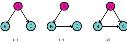
[image:3.612.327.549.245.321.2](a) (b) (c)
Fig. 1. Possible inference results of relationships among three variables (a) True/direct interactions, (b) indirect interaction inference, (c) bivariate inference.
set of observed data and their conditional dependencies. DBNs have been routinely applied to data, mainly long time series, to provide information about system dynamics. However, a major concern about DBNs is its inefficiency in large-scale prediction, i.e., with the presence of many variables.
Recently, a directed network inference approach, namely shrinkage vector autoregressive method (SVAR), was proposed by Rheinet al.[4] to circumvent the small sample problem. The basic procedure consists of first computing the shrinkage estimates of covariance matrices to obtain regression coeffi-cients for fitting autoregressive models. Then, instead of using the regression coefficients directly, the corresponding partial correlation coefficients are statistically tested. Significant co-efficients are selected using False Discovery Rate (FDR) [5] to be included into the reconstructed network.
Another recent advance in this area is the introduction of the concept of Granger causality (GC) [6], a statistical technique for causal inference well known in economics. Time series A is said to Granger cause time series B, if the forecast of B has incremental predictive power with the addition of A. The predictive power can be measured by the variances of residuals as a result of linear model fitting. Informally, the method measures the influence of one time series on another by checking if the prediction of the response can be improved by incorporating the knowledge of a predictor. Subsequently, for the application to gene expression data, one of the first attempts is a simple bivariate model that uses Granger causality to infer relationships between pairs of variables without taking into account other variables [7]. For
2009 Ninth IEEE International Conference on Bioinformatics and Bioengineering
978-0-7695-3656-9/09 $25.00 © 2009 IEEE DOI 10.1109/BIBE.2009.8
the purpose of our comparative experiments, we implemented a multivariate model in R, since the bivariate model could lead to false positive edges such as the ones in Fig. 1(c), compared with the true network (Fig. 1(a)).
All above three methods infer directed networks. One undi-rected but popular method, a shrinkage estimate method using graphical Gaussian models (GGMs), is proposed by Sch¨afer and Strimmer [8] to tackle the dimensionality problem. GGMs are undirected models which describe conditional dependence structure among variables. In essence, partial correlation is used as the mathematical foundation for establishing direct interactions among genes (Fig. 1(a)). When inferring the relationship between two temporal signals/gene expressions, the rest of the signals are also taken into account in the com-putation of partial correlation to discriminate between direct (Fig. 1(a)) and indirect (Fig. 1(b)) interactions. Significant coefficients of partial correlation can then be selected using FDR for the reconstruction of gene networks.
Although this method is fast and well suited for small sample data analysis [9], the inferred interactions are undi-rected. In an undirected network, the role that a gene plays in the regulatory activities is unknown. Therefore, based on partial correlation, we propose a directed approach specifically targeted at small-sample gene expression data. It is then compared with the existing directed inference methods as described above, DBNs, SVAR, and Granger causality, to demonstrate its effectiveness.
Although there are many comparative studies of interdepen-dence inference techniques in the literature [10], [11], few of them are conducted on microarray data sets. For example, in a comparative study on inference algorithms for multivariate time series interaction [10], GC is reported to perform well for stationary times series data, but is sensitive to non-linearity. The study was mainly based on neural data, which might be of completely different nature from gene expression data.
In contrast, our study focuses on the small sample problem in gene expression data analysis. This paper aims at illustrating the application of multivariate time series analysis in the reign of gene interaction inference. It also sheds light on the question of to what extend the model assumptions of individual algorithms influence the confidence of the inference outcome for biological networks. Specifically, we discuss the statistical properties of the transcriptional network and their impacts on the performance of an algorithm in the comparative evaluation. This paper is organised as follows. In the second section, we present the technical details of the three existing algorithms to be incorporated in the comparative analysis. Then in the third section a directed partial correlation algorithm for directed regulatory network inference is proposed. Experimental results and discussions are presented in the fourth section. The reported results indicate superior performance of the proposed algorithm in terms of both accuracy and efficiency.
II. RELATEDMETHODS
In this section, we first present the autoregressive models, since the three existing methods are based on them. Then, we
describe the technical details for three representative methods, focusing on their abilities in analysing gene expression data. Next, the proposed algorithm is formulated. These technical details provide us strong foundation for the discussions later on experimental results. Based on the interpretation of exper-imental results, we hope to shed some light on the nature of inference techniques, their advantages and inherent problems.
A. Existing multivariate time series inference methods
1) Vector autoregressive models (VAR): Suppose Y =
{yi|i = 1,2, ..., n} is a multivariate stationary time series consisting of nvariables andttime points. A p-order vector autoregressive VAR(p) model specifies that the value of the
ith variable at time pointt,yi(t), is a linear combination of a constant/mean value, the past of the multivariate time series, and a noise component
Y(t) =B+A
p
u=1
Y(t−u) +ε(t). (1)
B is a constant matrix of size n×t. ε consists of vectors of residuals {εi|i = 1...n}, each assumed to be zero mean noise with covariance matrix Σi. A is the n×n coefficient matrix representing the dynamic structure. When A is a constant matrix, this model assumes homogeneity across time. A special case of the p-order VAR process, the first-order autoregressive model (VAR(1)), is often considered when analysing microarray data for the sake of simplicity [3], [4]
Y(t) =B+AY(t−1) +ε(t). (2) 2) Granger causality inference method (GC):We start with Granger causality method (GC) in the multivariate case. Let
Y−symbolise the past state ofY,Y−={Y(u)|u= 1, ..., t−
1}, and lety−i symbolise the past of variableyi. The Granger causality measure of prediction power of one variable yi on the other variableyj,i=j, is defined by
gyi→yj = ln
σyj|Y−
σy
j|Y/i−
. (3)
Symbol “|” denotes operation “condition on” and symbol “/” denotes “without”.σyj|Y− is the variance of the residualε(t) in the VAR(1) model for yj conditioned on the past of all variablesY−. It is compared toσy
j|Y/i− which is conditioned on the past of all variables butyi,Y/i−. GC directly measures the prediction power ofyi foryj, as a result of the reduction of prediction errors by incorporatingyiinto the VAR(1) model foryj. In other words, if introducingyi significantly reduces the variance of the prediction error of yj, then a variable
yi Granger causes the variable yj. Since it requires fitting autoregressive model with all variables and their past states, GC can only be applied to data satisfying: t > n(p+ 1), indicating its limited potential in gene expression analysis.
3) Shrinkage VAR method (SVAR): Although the VAR model has been widely used in economics and neuroscience, it has its own limitations when small samples are encountered. An effective shrinkage estimation procedure was developed for learning the VAR models from small sample data [4]. The idea is that a shrinkage estimate can replace the covariance matrix for the joint matrix of both the present data and the lagged data, which then leads to the computation for regression coefficients. The covariance matrix would be otherwise ill-conditioned, given the large number of variables (2×n) and short time seriest, tn.
Let Φ denote the joint matrix of the multivariate Y’s present state (Y+ = {Y(u)|u = 2, ..., t}) and past state (Y−={Y(u)|u= 1, ..., t−1}),Φ = [Y+Y−]. Assuming that the data has zero mean, an unbiased estimate of the covariance matrix for Φis
cov(Φ) = 1
t−1[Y+Y−][Y+Y−] (4)
=t−11
Y+
Y+ Y+
Y− Y−
Y+ Y−
Y−
.
Note that this matrix contains the sub-matrices Y−Y− and
Y−
Y+. Meanwhile, the ordinary least squares (OLS)
estima-tion [12] for the regression coefficientAin the VAR(1) model (Eq.(2)) is:
ˆ
A(1)= (Y−
Y−)−1Y−
Y+. (5)
Therefore, the shrinkage estimation ofcov(Φ)will lead to the estimated coefficient matrix Aˆ. Then the partial correlation coefficientsqcan be computed fromAˆand the FDR is used to select significant coefficients. With large number of variables, this method gave good result in the comparative simulation study using simulated autoregressive data in the original paper [4].
4) Dynamic Bayesian networks inference method (DBNs): DBNs implementations are usually designed for data with hundreds or thousands of samples. The limitation of microar-ray experimental costs prohibits most of the techniques from exploring small sample gene expression data. In this paper, we use the implementation of the R package G1DBN [3], which is based on a trivariate AR(1) model:
Y(1) ∼ N(μ1,Σ1), (6)
Y(t) = B+AY(t−1) +ε(t), ε(t) ∼ N(0, σ),
with predefined μ1,Σ1, and σ. This method measures the conditional dependence between two variablesyi, yjby testing the null hypothesisH0i,j,k: “aij|k= 0”on every third variable
{yk|k = i, j}. Then, a score is assigned to the potential edge yi → yj corresponding to the maximum p-values from the tests pmax(yi → yj). This means the algorithm has a computational complexity ofO(n3). The computation of this method may be too heavy for data with more than a hundred variables. Since the simulated data are generated following the characteristic assumption of small sample, we hope to cast light on this particular aspect.
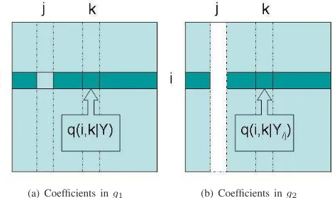
[image:5.612.322.556.75.215.2](a) Coefficients ing1 (b) Coefficients ing2
Fig. 2. Partial correlation matrices before and after deletingyj. To predict yj’s influence onyi, partial correlation coefficients are selected into group testing and coloured dark green.
III. PROPOSED DIRECTED PARTIAL CORRELATION INFERENCE METHOD(DPC)
The shrinkage estimate for partial correlation in [8] was for-mulated specifically for the inference from small sample gene expression data. Although partial correlation is undoubtedly fast in computation and suitable for small sample problem, it can only infer undirected networks. Another problem is, variable time lag cannot be taken into account as in a VAR(1) model. We introduce the notion of directed partial correlation (DPC) for fast inference of directed gene networks. The idea is similar to the idea behind Granger causality - a variable A has causal influence on another variable B, if the removal/addition of A has a large impact on the prediction of B. While GC measures this impact by comparing the residuals before and after adding A to the prediction of B, DPC measures it by examining the correlation coefficients.
A. Zero-order directed partial correlation DPC(0)
Directed partial correlation aims to investigate the effect of including a variable into the predictions of another gene, i.e. the change of partial correlations among other genes. Let
QY of size n×n denote the partial correlation matrix for
Y. Each element q(i, j|Y) in QY is the partial correlation between yi and yj givenY, i = 1, ...n, j = 1, ..., n, i = j, i.e., the correlation betweenyi andyj after the linear effects of the rest of variables are removed. This can be formulated asq(i, j|Y). Removal of linear effects from others means that resulting partial correlation indicates the direct relationship between two variables. Fig. 2(a) shows q(i, k|Y), k = i, j, which denotes the partial correlation betweenyi andykwhen effects from all others, includingyj, are removed.
However, relationship indicated byq(i, j|Y)is undirected. To investigate the influence yj has on yi, we propose the following. If we delete the variable yj from Y, the partial correlation between yi and another variable yk, k = i, j is denoted as q(i, k|Y/j)in the matrixQY/j. As shown in Fig. 2(b), in the prediction of relationship betweenyiand any other variableyk,k =i, j,q(i, k|Y/j)no longer remove the effect fromyj, which meansyjno longer take part in the prediction
ofyi. Consequently, there are two groups of statistics related to the prediction ofyi, each corresponding to coefficients before and after the removal of yj. To be more specific, the first group is theith row inQY without theith and jth element,
g1 = {q(i, j|Y), j = i}, shown in dark green in Fig. 2(a). The second group corresponding to the dark green elements in Fig. 2(b) is theith row in QY/k without the ith element,
g2= {q(i, j|Y/k), j =i, k}. Both groups have the length of
n−2. The effectyj has on the prediction ofyiis defined as:
e(0)
yj→yi
=t-test(g1, g2) (7) =t-test{q(i, k|Y)|k=i, j},{q(i, k|Y/j)|k=i, j}. We use Student’s t-test on the two groups to see if there exists an effect on the prediction of other variables with the removal of variableyj. The null hypothesis is that there is no significant difference between the two groups, before and after the removal. Student’s-t test compare the sample means:
τ = g¯1−g¯2
(n−2)−1(σ2
g1+σg22)
, (8)
whereσg1stands for the standard deviation ofg1, the denom-inator ofτ is the standard error of the difference between two means, the degree of freedom for the test is2n−6.
In summary, we take advantage of the fact that in computing partial correlation between two variables, all effects from other variables need to be removed. In other words,yj takes part in the predictions ofyi with all other variables yk. We measureyj’s influence onyi by comparing partial correlation coefficients related to yi before and after the deletion of yj, sinceyj does not take part in the prediction of yi after the deletion.
B. First-order directed partial correlation DPC(1)
A key feature of the proposed DPC method is that it can be easily extended to include time lags. The correlation between the variables measured as a function of time lag is of interest because such a time lag may reflect a causal relationship. Let Φ be the joint matrix of the present state and the past state of data,Φ = [Y+Y−]. To compute the correlation matrix for Φ, we note that the covariance matrix of Φis ill-conditioned for small sample data and therefore not suitable. We use the shrinkage estimate method in Eq.4 to compute the partial correlation matrixQ(1)Y forΦ:
Q(1)Y =
Q++ Q+−
Q−+ Q−−
. (9)
Hence each element in the sub-matrixQ++,q(1)(i, j)withi= 1...n, j = 1...n, stands for the partial correlation between yi andyj, when the effects of the present states of other variables and the past states of all variables are removed. If a variable
yjis deleted from the joint matrixΦ, the corresponding partial correlation matrixQ(1)Y/j has equivalent meaning as described in the zero-order model, i.e. the effect ofyj is not taken into
account in the prediction of the other variables. The first-order directed partial correlation fromyjtoyican be formulated as:
e(1)
yk→yi (10)
=t-test
{q(1)(i, j|Y)|j= i},{q((1)i, k|Y
/j)|k=i, k}
.
Note that although the partial correlation matrix is of size 2n×2n, only the sub-matrixQ++is used for computinge(1). The probability of the directed interaction is indicated by the
Algorithm 1First-order directed partial correlation (DPC(1)) Construct the joint matrix Φ = [Y+Y−], with Y+ the present state (Y+ = {Y(u)|u ∈ 2...t}) and Y− the past state (Y−={Y(u)|u∈1...t−1});
Compute the partial correlation matrix Q(1)Y for the joint matrixΦ;
foreach variableyk in Y do
Compute the partial correlation matrixQ(1)Y/k for the joint matrix withyk removedΦ/k;
foreach variableyi, i=k do
Compute the influence ofyk on yi,eki, according to Eq.(1);
end for end for
foreach diagonal elementeii in the directed partial corre-lation score matrix do
Compute the partial correlation matrixQ(1)Y
/i for the joint matrix with the lagged datayi−removedΦ/i−;
Compute the effect ofy−i on yiaccording to Eq.(1).
end for
resultantp-values. Using FDR, adjustedp-values are selected in accordance to confidence levels, for example,2% of FDR means accepting all tests with adjusted p-values < 0.02 as significant.
Conceptually, DPC tests the effect of one variable on the predictions of another by all the rest of variables at the same time, hence is able to monitor the dynamic process within reasonable computation time. It avoids linear model fitting, thus is more efficient and less constrained by the sample size.
IV. EXPERIMENTS
Previously, SVAR and DBNs were experimentally proved to be useful using simulated data from autoregressive models [3], [4]. These methods are based on the autoregressive model and their performance on other types of data is still not clear. When the data satisfy the model assumption, we can expect the corresponding technique to perform well. Therefore, an important question pertains to which assumption best describes gene expression data. In this section, we aimed at investigating the following question: how well the inference methods can meet the requirements of microarray data.
Since real expression data are generally noisy, they may not be fully reflective of the gene relationships and the ground truth is unknown, comparisons of performance are conducted
TABLE I
SIMULATED SMALL SAMPLE DATA SETS CONFIGURATION FOR NETWORKS OF VARIOUS SIZES
Data set Network size Sub-network Sample Noise
selection size level
1 10 20 30 40 50 80 100 120 150 180 200 220 250 280 300 clustAdd 25 8%
2 10 20 30 40 50 80 100 120 150 180 200 220 250 280 300 clustAdd 25 5%
3 10 20 30 40 50 80 100 120 150 180 200 220 250 280 300 clustAdd 25 3%
4 10 20 30 40 50 80 100 120 150 180 200 220 250 280 300 clustAdd 15 6%
5 10 20 30 40 50 80 100 120 150 180 200 220 250 280 300 clustAdd 15 4%
6 10 20 30 40 50 80 100 120 150 180 200 220 250 280 300 clustAdd 15 2%
with synthetic data. SynTReN is well suited for testing module network algorithms [13]. By using topologies generated based on previously described source networks, SynTReN allows good approximation of the statistical properties of real bio-logical networks.
Four multivariate time series inference algorithms as de-scribed above are evaluated in this experiment. Their ways of inferring the final network vary and each requires fine tuning for the parameters, which could be subjective for large-scale experiments (in the synthetic data experiment altogether 142 data sets are used). To eliminate any subjective element and enable a fair comparison, we decide to compare directly on their preliminary output, the score matrices. For clarity, the related symbols for each score matrix in the algorithms’ technical details are listed in Table II.
For the inferred score matrices, we compute their true positives (TP), false positives (FP), true negatives (TN), and false negatives (FN) given a threshold. This procedure was repeated 500 times for each test statistic and variance sce-nario, to obtain Receiver Operator Characteristic (ROC) curves [14], [15] for describing the dependence of true positive rate/sensitivity T P R= T P/(T P +F N) and false positive rate/specificityF P R=T N/(T N+F P). ROC curves provide a straightforward graphical representation of the performance of the algorithms, hence are especially useful in statistically principled comparisons. It avoids issues related to a chosen threshold, by using all possible thresholds. As a summary metric for ROC, the area under the ROC curve (AUC), as its name indicates, can measure the average accuracy of the prediction.
While AUC provides quantitative measurement on average performance for a method, maximum F-score [16] evaluates each method at its point of optimum. F-score is the harmonic mean of precision (T P/(T P+F P)) and recall (T P/(T P+
F N)). As a composite measure, F-score challenges algorithms with higher specificity and benefits algorithms with higher sensitivity. Both of the metrics are used when appropriate in the following experiment section. Apart from these metrics, we also base our evaluation on the the consumed computation time and the true positive rate at the point of 0.2 false positive rate, since usually a low false positive rate is preferred.
SynTReN produces synthetic transcriptional regulatory net-works and the corresponding simulated microarray data sets, parameterized by the network topology, size of the net-work/number of genes, levels of biological, experimental, and
input noise etc. Network topologies can be generated by selecting sub-networks from previously described biological networks or by using random graph models. The former method is used here to offer better approximation. Two dif-ferent strategies to select a connected subgraph are imple-mented: neighbour addition (neighAdd) and cluster addition (clusterAdd). It was suggested that sub-network selection by cluster addition is preferable [17], since the resulting sub-network preserves features of scale-free sub-networks such as having hubs. However, consider that during variable selection process one may not include all neighbours of a hub gene, sub-networks by neighbour addition may sometimes represent a more realistic situation in gene network analysis. Hence we use both strategies in simulated data generation.
After the topologies of the synthetic networks are sampled, transition functions can be determined and enzyme kinetic equations are selected for each gene and its regulators. Com-bined with external conditions that trigger the network, the expression levels of genes in each experiment are generated according to the activities of their regulators. The final data generated by SynTReN are quantiled to the range of [0,1] where 0 indicates no expression and 1 indicates maximal expression. We normalize the data to thelog2ratio by selecting one of the samples as the control.
We design three sets of experiments in order to assess the methods’ performance in a coherent manner. In the first and second experiment, data sets of small sample, varying network sizes and data sets of large network, varing sample sizes are generated. In the third experiment, sample size slightly larger than network size/gene number are generated. However in the first experiment, data sets are analysed by DPC, SVAR and DBNs but not GC, since GC requires sample size larger than network size (n < t).
The experiments are designed to give a thorough evaluation of the proposed algorithm, to observe its performance in different scenarios, to compare four algorithms in a coherent manner. Specifically, we note that settings in the first exper-iment are perhaps closest to realistic situation for microarray data analysis, and therefore results from the first experiment should receive careful consideration and interpretation.
A. Networks of various sizes and small sample size
In this experiment, we assess the influence of network size on the performance of inference algorithms, by fixing the sample size to a small number and vary the network size.
0.0
0.2
0.4
0.6
0.8
1.0
Network size
AUC
10 20 30 40 50 80 100 150 200 250 300
DPC(1) DPC(0) SVAR DBNs
(a)
0.0
0.2
0.4
0.6
0.8
1.0
Network size
AUC
10 20 30 40 50 80 100 150 200 250 300
DPC(1) DPC(0) SVAR DBNs
[image:8.612.66.278.91.441.2](b)
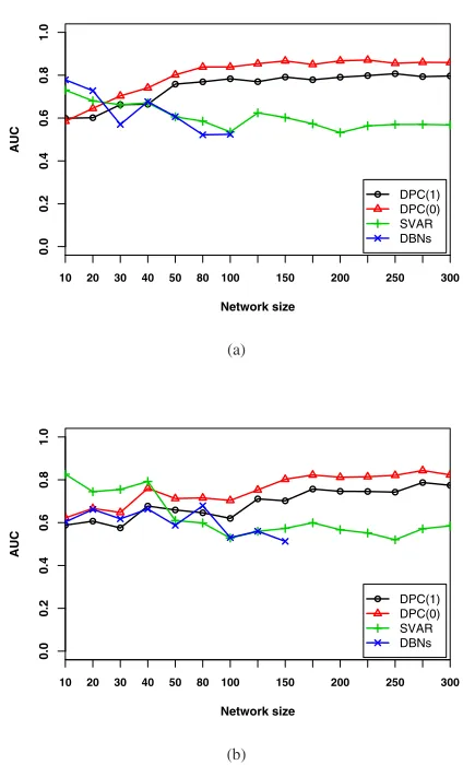
Fig. 3. The AUC values for three network inference algorithms on different data sets with noise level at about 5% on average (a) fixed sample size of 25, network size/gene number10∼300, (b) fixed sample size of 15, network size/gene number10∼300.
This means GC cannot be applied in this experiment, since it requires long time series (t n) to fit linear models. First, E.colisub-networks are selected by cluster addition as the network topologies. We generate altogether 45 data sets with 25 samples varied in network size from 10 nodes to 300 nodes, and 45 data sets with 15 samples varied in network size from 10 nodes to 300 nodes. The configurations in the network topology selection, sample size and network size are provided in Table I. In this table, parameter noise level refers to all the noise parameters in SynTReN: levels of biological, experimental, and input noise. They are set to the same value. The noise level is set relatively lower for the 15-sample data sets than the 25-sample data sets.
For each algorithms, the resulting AUC values for data set 1, 2 and 3 are averaged and plotted in Fig. 3(a), so are the inference results for data sets 4, 5, and 6 in Fig. 3(b). Because of the computation costs of DBNs, we only compute results for networks of size10∼100for the 25-sample data and size
10∼150for the 15-sample data. The plots show the effect of the amount of available gene expression data on the inference results. Although SVAR and DBNs sometimes outperform DPC with smaller networks/less variables, when faced with increasing network size, their performance both drops rapidly when there are only small amount of data available. However, DPC’s overall performance dramatically improves from the beginning, i.e. for smaller networks. Then it stays the same regardless of the changes in network size.
Generally, the performance of most of the algorithms de-grades as the number of genes increase. This conforms to current theory. In contrast, DPC outperforms others only when the network size is big enough. However, this is reasonable. The two-sample test DPC based on is effective only when there are big enough sample populations, which, in this scenario, are equivalent to the number of genes/variables. In summary, DPC shows superior performance in inferring large-scale gene networks, although for small networks it is sometimes outper-formed by SVAR and DBNs.
B. Networks of fixed size and various sample sizes
To assess the influence of sample size on the performance of the inference algorithms, we generate data sets for a fixed network size but of various sample sizes. Four E.coli sub-networks selected by cluster addition of size 50, 50, 100, and 100 genes were chosen as the network topologies. For each of the two 50-gene networks, we generate 12 gene expression data sets with sample sizes varied from 60 to 1000. For each of the two 100-gene networks, we generate 8 data sets with sample sizes varied from 120 to 1000. Altogether 40 data sets are generated and used as input for the four algorithms. The resulting AUC values for the two 50-gene networks are averaged and plotted in Fig. 4(a) and the same for the resulting AUC values from two 100-gene networks plotted in Fig. 4(b). All algorithms show different behaviours when faced with increased amount of data. In Fig. 4(a), the performance of all methods improve as the sample size grows at the beginning (60∼180 samples), but then level off eventually. Compared with the AUC values for DBNs and DPC, the AUC values for SVAR and GC show larger variations. The best performer in this case when the network size is 50 genes is DBNs, followed by DPC(0).
However, this situation is reversed when the network size is increased to 100 genes. Performance of DBNs drops sharply, reflecting its sensitivity to the network size. Interestingly, the performance of DPC improves dramatically compared to that in the case of 50-genes. With bigger network/more variables, one would expect a decent in the performance of inference methods. DPC, in contrast, perform even better, which conform to the conclusion and interpretation for DPC in the first experiment.
With increasing number of samples, the improvement of performance is not as dramatic as one would expect in the case of 50-gene networks. A performance plateau was reached at 180 samples for most of the algorithms. However, the case with 100-gene networks are quite different in that general
0.0
0.2
0.4
0.6
0.8
1.0
Sample size
AUC
60 80 100 120 150 180 200 250 300 400 500 1000
DPC(1) DPC(0) SVAR GC DBNs
(a)
0.0
0.2
0.4
0.6
0.8
1.0
Sample size
AUC
120 150 180 200 250 300 500 1000
DPC(1) DPC(0) SVAR GC DBNs
[image:9.612.317.558.69.314.2](b)
Fig. 4. The AUC values for four network inference algorithms on different data sets with noise level at 10% (a) fixed network size of 50 genes, sample size60∼ 1000, (b) fixed network size of 100 genes, sample size120∼ 1000.
performance only starts to improve when more than 300 samples are available. An exception is DPC, which show fairly steady performance across all sample sizes.
From this experiment we can observe that expecting dra-matic improvement in the performance of inference algorithms by increasing sample size is unrealistic, especially for microar-ray data whose samples are costly. Again DPC outperforms other algorithms for larger networks.
C. Networks of typical sizes
In the third experiment, we investigate the situation when the network size is selected to be slightly smaller than the sample size. This is close to a scenario when a researcher chooses the number of genes to be included in the network according to the number of microarray samples available. Four data set configurations with 50 genes×100 samples, 80 genes×100 samples, 100 genes×150 samples, 150 genes×180 samples are considered. Three data sets are generated for each configuration. By assigning different random seeds to
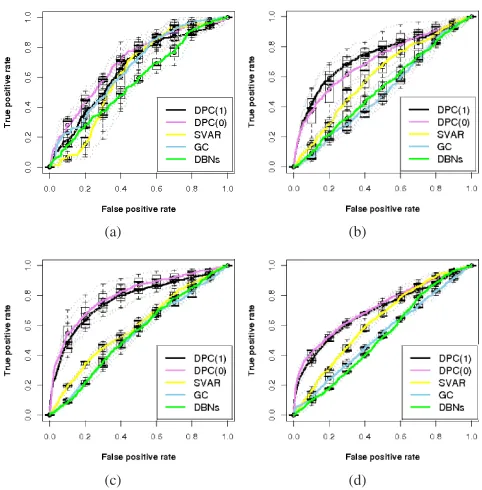
(a) (b)
(c) (d)
Fig. 5. ROC curves for the comparisons of the four network inference algorithms using their score matrics, (a) synthetic network of 50 genes and 100 samples, (b) synthetic network of 80 genes and 100 samples, (c) synthetic network of 100 genes and 150 samples, (d) synthetic network of 150 genes and 180 samples.
TABLE II
PERFORMANCE OF THE FOUR MULTIVARIATE TIME SERIES INFERENCE ALGORITHMS ON GENE NETWORKS OF TYPICAL SIZES
Method DPC(1) DPC(0) SVAR GC DBNs
Score matrix e(1) e(0) |r| g pmax
Data size Average AUC value
50×100 0.65 0.70 0.62 0.60 0.57
80×100 0.79 0.76 0.65 0.57 0.55
100×150 0.79 0.79 0.58 0.55 0.53
150×180 0.70 0.72 0.63 0.53 0.53
Data size Average true positive rate (false positive rate=0.2)
50×100 0.37 0.44 0.25 0.34 0.28
80×100 0.60 0.58 0.28 0.20 0.25
100×150 0.64 0.67 0.24 0.45 0.24
150×180 0.56 0.60 0.31 0.27 0.22
Data size F scores
50×100 0.11 0.14 0.06 0.15 0.07
80×100 0.18 0.22 0.05 0.18 0.05
100×150 0.20 0.23 0.05 0.20 0.04
150×180 0.18 0.21 0.05 0.09 0.03
Average time (min)
50×100 1.0 0.3 0.3 38.2 84.3
80×100 1.4 0.5 0.3 56.9 136.5
100×150 1.8 0.7 0.3 67.3 173.2
150×180 2.5 0.9 0.4 88.9 230.5
SynTReN to select random nodes as a starting point, all data sets are guaranteed to relate to different network topologies. The noise level for all the noise parameters (e.g. biological noise and experiment noise) in SynTReN is set to 10%.
To evaluate the performance of the four algorithms, we first
[image:9.612.323.548.412.636.2]plot the resulting ROC curves in Fig. 5 individually for the four scenarios. In each plot, for each algorithm, its results on all three data sets are first plotted as the dotted curves, then their boxplots are used as the summary curves.
It is easy to observe, for SVAR, GC and DBNs, a descent in their performances as network expands. In contrast, DPC shows robustness to network size in this case, when sample size is reasonable in comparison to the network size.
Quantitative measurements of performance including AUC values, true positive rates, F scores and average computation time for each methods are provided in Table II, with best results bolded. For clarity, score matrices are the symbols corresponding to the technical details in the previous section. The average performance are reported as a result of using three data sets for each typical data size. AUC values are calculated from Fig. 5, and the average true positive rates are given for each algorithm when the false positive rate is 20%. Average consumed time is for a PC (Intel Pentium 4 2.80GHz). From this table, noticeable advantage to DPC can be seen in terms of both accuracy and efficiency, although SVAR is the most efficient.
V. CONCLUSIONS
This paper reviews some recent advances on multivariate time series inference in the field of gene expression data analysis and reports a new method, aiming at shedding light on future research. We performed thorough experiments to inves-tigate the properties of the proposed method and other methods in comparison, although settings for the first experiment are closer to realistic situation for microarray data.
Superior performance of the proposed directed partial cor-relation (DPC) for large-scale network inference is observed throughout the experiments. Its excellent property of robust-ness to gene number/network size is made explicit in the first experiment, while other methods in comparison show fast descent in their performance. Moreover, there is no obvious effect of the sample size on the performance of inference algorithm, as it is shown in the second experiment. The marginal influence on the inference results by increasing sam-ples to a realistic limit indicates that, exploring fundamental advancement in inference algorithms is perhaps the key to success in this field.
Finally, we note that a major difference between SVAR and DPC is, SVAR inspects the regression coefficients of the full linear model, while DPC takes advantage of the idea behind Granger causality and tests the effect on the removal of individual variables. Unlike the method using Granger causality, the computation cost for DPC is low and not substantially affected by network size. Following the success of DPC on synthetic data, we would like to test it on real biological data and this will be our new line of investigation in the near future.
REFERENCES
[1] R. Clarke, H. W. Ressom, A. Wang, J. Xuan, M. C. Liu, E. A. Gehan, and Y. Wang, “The properties of high-dimensional data spaces: implications
for exploring gene and protein expression data,” Nature Revolution Cancer, vol. 8, no. 1, pp. 37–49, 2008.
[2] A. Bernard and A. J. Hartemink, “Informative structure priors: joint learning of dynamic regulatory networks from multiple types of data.”
Proceedings of the Pacific Symposium on Biocomputing, pp. 459–70, 2005.
[3] S. Lebre, “Inferring dynamic genetic networks with low order indepen-dencies,” 2007.
[4] R. Opgen-Rhein and K. Strimmer, “Learning causal networks from systems biology time course data: an effective model selection procedure for the vector autoregressive process,”BMC Bioinformatics, vol. 8, no. Suppl 2, p. S3, 2007.
[5] Y. Benjamini and Y. Hochberg, “Controlling the false discovery rate: A practical and powerful approach to multiple testing,”Journal of the Royal Statistical Society, vol. B, no. 57, pp. 289–300, 1995.
[6] C. W. J. Granger, “Investigating causal relations by econometric models and cross-spectral methods,”Econometrica, vol. 37, pp. 424–438, 1969. [7] N. D. D. Mukhopadhyay and S. Chatterjee, “Causality and pathway
search in microarray time series experiment.”Bioinformatics, 2006. [8] J. Sch¨afer and K. Strimmer, “An empirical Bayes approach to inferring
large-scale gene association networks.”Bioinformatics, vol. 21, no. 6, pp. 754–64, 2005.
[9] D. Veiga, F. Vicente, M. Grivet, A. de la Fuente, and A. Vasconcelos, “Genome-wide partial correlation analysis of escherichia coli microarray data,”Genet. Mol. Res., vol. 6, no. 4, pp. 730–742, 2007.
[10] M. Winterhalder, B. Schelter, W. Hesse, K. Schwab, L. Leistritz, D. Klan, R. Bauer, J. Timmer, and H. Witte, “Comparison of linear signal processing techniques to infer directed interactions in multivariate neural systems,”Signal Processing, vol. In Press, Uncorrected Proof, 2005. [11] E. Pereda, R. Q. Quiroga, and J. Bhattacharya, “Nonlinear multivariate
analysis of neurophysiological signals,” 2005.
[12] R. Bro, N. D. Sidiropoulos, and A. K. Smilde, “Maximum likelihood fit-ting using ordinary least squares algorithms,”Journal of Chemometrics, vol. 16, pp. 387–400, 2002.
[13] T. Michoel, S. Maere, E. Bonnet, A. Joshi, Y. Saeys, T. Van den Bulcke, K. Van Leemput, P. van Remortel, M. Kuiper, K. Marchal, and Y. Van de Peer, “Validating module network learning algorithms using simulated data,”BMC Bioinformatics, vol. 8, no. Suppl 2, 2007.
[14] J. Egan,Signal detection theory and ROC analysis, Series in Cognition and Perception. New York, NY, USA: Academic Press, 1975. [15] T. Fawcett, “An introduction to ROC analysis,”Pattern Recogn. Lett.,
vol. 27, no. 8, pp. 861–874, 2006.
[16] C. J. V. Rijsbergen, Information Retrieval. Newton, MA, USA: Butterworth-Heinemann, 1979.
[17] T. V. den Bulcke, K. V. Leemput, B. Naudts, P. van Remortel, H. Ma, A. Verschoren, B. D. Moor, and K. Marchal, “SynTReN: a generator of synthetic gene expression data for design and analysis of structure learning algorithms.”BMC Bioinformatics, vol. 7, no. 1, p. 43, 2006.