University of Warwick institutional repository: http://go.warwick.ac.uk/wrap
This paper is made available online in accordance with
publisher policies. Please scroll down to view the document
itself. Please refer to the repository record for this item and our
policy information available from the repository home page for
further information.
To see the final version of this paper please visit the publisher’s website.
Access to the published version may require a subscription.
Editor(s): Turgay Çelik and Tardi Tjahjadi
Book Title: Multiscale texture classification and retrieval based on
magnitude and phase features of complex wavelet subbands
Year of publication: 2011
Link to published item:
http://dx.doi.org/10.1016/j.compeleceng.2011.06.008/
Publisher statement: “NOTICE: this is the author’s version of a work
that was accepted for publication in Computers & Electrical
Engineering. Changes resulting from the publishing process, such as
peer review, editing, corrections, structural formatting, and other quality
control mechanisms may not be reflected in this document. Changes
may have been made to this work since it was submitted for
Multiscale Texture Classification and Retrieval Based on Magnitude and Phase
Features of Complex Wavelet Subbands
Turgay Celik, Tardi Tjahjadi
School of Engineering, University of Warwick, Gibbet Hill Road, Coventry, CV4 7AL, United Kingdom.
Email: [email protected]
Abstract
This paper proposes a multiscale texture classifier which uses features extracted from both magnitude and phase responses of subbands at different resolutions of the dual-tree complex wavelet transform decomposi-tion of a texture image. The mean and entropy in the transform domain are used to form a feature vector. The proposed method can achieve a high texture classification rate even for small number of samples used in training stage. This makes it suitable for applications where the number of texture samples used in training is very limited. The superior performance and robustness of the proposed classifier is shown for classifying and retrieving texture images from image databases.
Keywords:
Texture classification, texture retrieval, multiscale analysis, feature extraction, dual-tree complex wavelet transform, discrete wavelet transform.
1. Introduction
Content-based image retrieval (CBIR) from unannotated image databases has been gaining interest of the research community due to tremendous growth in size of online digital images. A typical CBIR system consists of two main parts: 1) feature extraction and 2) similarity measurement. First, features such as shape, texture and colour, which constitute the image signature are generated to represent the content of a given image. The similarity of a query image to the images in database is then measured using an appropriate distance metric.
The ability to classify texture, where texture is used to represent the content of an image, is a fundamental requirement of a CBIR system. For texture classification Gabor filters, wavelet transforms, finite impulse response filters have been widely used. The Gabor filter is appealing because of its simplicity and support from neurophysiological experiments [1]. Gabor filters have been used for texture segmentation despite being based on texture reconstruction [2], [3]. A general Gabor filter bank is often too large since it is designed to capture general texture properties. However, textures can be classified using a small set of filters, which gives rise to the filter selection problem. The wavelet based texture classifiers are similar to Gabor based methods with the Gabor filters replaced by the Discrete Wavelet Transform (DWT) [4, 5, 6, 7, 8, 9]. The DWT based methods employ multiscale decomposition to extract high-frequency components from wavelet subbands for texture representation. However the DWT is shift variant, thus a shift in the signal degrades the performance of DWT based classifiers.
DWT has also been used for texture retrieval. For example, the generalized Gaussian distribution (GGD) and Kullback-Leibler distance metrics have been used in the DWT domain [10]. The similarity measure and feature extraction are jointly considered for the estimation and detection in a maximum likelihood framework, providing a definition for similarity measurement using Kullback-Leibler divergence (KLD). The performance of the texture retrieval system then depends on modelling the marginal distribution of wavelet coefficients using GGD and on the existence of a closed form for the KLD between GGDs. DWT has limited directionality, i.e., wavelet subbands are oriented at directions of 0◦, 45◦ and 90◦ at each scale of
However, DWT is not robust to shift [11] which means that small shifts in the input signal can cause major variations in the distribution of energy between DWT coefficients at different scales. This makes it difficult to use features extracted from DWT coefficients in supervised pattern classification applications. Since the wavelet filters of DWT are separable and real, DWT has poor directional selectivity for diagonal features because [11]. These characteristics are major obstacles for robust feature representation. The shift invariance can be achieved by using the undecimated form of the dyadic filter tree but this suffers from increased computation requirements and high redundancy in the output information. Gabor wavelets can be used as an alternative to DWT. They are designed to be directionally selective and are robust to shift since they are non-decimated, but they are therefore overcomplete and hence computationally expensive. The dual-tree complex wavelet transform (DT CWT) has been shown to be approximately shift invariant and has limited redundancy [11]. They have good selectivity and directionality in 2-dimensions (2-D) with Gabor-like filters. The DT CWT has efficient order-N computation which is only 4 times the simple DWT for image processing.
The afore-mentioned advantages of DT CWT and its multiscale structure make it appealing for texture classification and retrieval [12]. In our recent work, we used DT CWT subbands to design a multiscale texture classifier [13]. The classifier uses simple statistical features of the mean and standard deviation of the magnitude of DT CWT subbands in different scales. The multiscale classifier is further improved by employing Bayesian inference [14]. The dimensionality of multiscale feature vectors is reduced using principal component analysis (PCA). The class conditional probability density function of low-dimensional feature vectors for each texture class is then estimated by using Parzen-window estimate with identical Gaussian kernels and is used to represent the texture class. A query texture image is classified as the corresponding texture class with the highest a posteriori probability according to a Bayesian inferencing. Performance gain with respect to the classifier in [13] is achieved at the expense of higher computational complexity. The inter-scale phase relationships of complex transform coefficients are also studied and a wrapped Cauchy or von Mises distribution is utilised to model the relative phase distributions [15]. The phase and magnitude information of the complex wavelet coefficient are combined into a real measure to describe the intensity variation of a texture [16]. The measure is modelled with the real generalized Gaussian distribution (GGD) and the model parameters are used as the texture feature during the classification [16]. However, the model based methods share a general problem of computational complexity in fitting the model to the data extracted from DT CWT decompositions.
In this paper, we show that texture classification without a complicated model can be achieved by using simple statistical measures extracted from magnitude and phase of DT CWT subbands. We improve the performance of our previous work [13] by using both magnitude and phase of the complex subbands of DT CWT. The additional information provided by the phase combined with the magnitude of the complex subbands results in more discriminative feature vectors. We also modified the texture feature vector structure to increase its discriminability. The new classifier is applied to both supervised texture classification and texture retrieval problems.
The paper is organized as follows. Section 2 presents DT CWT. Section 3 presents the proposed multiscale texture classifier, the learning and classification of texture features for different texture classes, and the process of texture retrieval. The experimental results and discussions are presented in Section 4. Finally, Section 5 concludes the paper.
2. Dual-tree complex wavelet transform
The DWT is not shift invariant due to the decimation during the transform. A small shift in the input signal generates very different wavelet coefficients. The DT CWT [11] exhibits approximate shift invariance and improved directional resolution. It achieves perfect reconstruction and good frequency characteristics using two parallel fully decimated trees with real coefficients. The one-dimensional (1-D) DT CWT is implemented using a pair of filter banks operating on the same data simultaneously as shown in Figure 1. The upper iterated filter bank (denoted with indexa) represents the real part of a complex wavelet transform, meanwhile the lower one (denoted with indexb) represents the imaginary part. There are two sets of filters used, the filters at level 1, and the filters at all higher levels.
Figure 1: Implementation of the 3-level 1-D DT-CWT using two filter banks operating as two parallel trees on the same data, whereH0i andH00i are low-pass wavelet filters andH1iandH01i are high-pass wavelet filters. The outputs from the upper and lower trees are interpreted as the real and imaginary parts of the DT CWT coefficients, respectively.
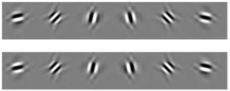
Figure 2: The real (top row) and imaginary (bottom row) parts of the impulse responses of the DT CWT filters for the 6 directional subbands, all illustrated at level 4 of the transforms. The complex wavelets provide 6 directionally selective filters. From left to right, 15◦, 45◦, 75◦,
[image:4.595.184.411.551.641.2]Input
Wavelets Level 1
Level 2
Level 3
Level 4
Scaling fns Level 4
(a)
Input
Wavelets Level 1
Level 2
Level 3
Level 4
Scaling fns Level 4
(b)
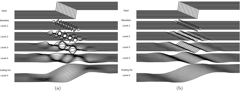
Figure 3: (a) Shift dependence of the DWT: signal reconstructions from wavelet and scaling function components at levels 1 to 4 of the DWT decompositions of 16 shifted step responses; and (b) Shift invariance of the DT-CWT: signal reconstructions from wavelet and scaling function components at levels 1 to 4 of DT-CWT decompositions of 16 shifted step responses.
To better understand the shift dependence of the DWT, an input signal consisting of a step function at sixteen different shifts is decomposed using a four level DWT as shown in Figure 3(a). In each case, the input is a unit step, shifted to 16 adjacent sampling instants in turn. Each unit step is passed through the forward and inverse version of the DWT. The figure shows the input steps and the components of the inverse transform output signal, reconstructed from the wavelet coefficients at each of levels 1 to 4 in turn and from the scaling function coefficients at level 4. Summing these components reconstructs the input steps perfectly. The 4-level DWT decomposition of 1-D signalX produces real-valued high-pass subbands ofX1,1, X2,1, X3,1, X4,1, and real-valued low-pass subband X4,0 at the final level of decomposition. The
reconstructed signals shown in the second row of Figure 3(a) are reconstructions only from subbandsX1,1
andX4,0with the other subbands set to 0, i.e.,X2,1= 0,X3,1= 0, andX4,1= 0. Similarly, the third, fourth,
and fifth rows are reconstructed only fromX2,1 andX4,0, X3,1 andX4,0, andX4,1 andX4,0, respectively.
The signals in the last row is reconstructed only from X4,0. If the the transform is shift invariant, then
the reconstructions from the same subbands should be similar shape. However, the shift dependence of the transform is evident from the varying energy in each of the reconstructed signal. To demonstrate the shift invariance of the DT CWT, the same procedure is applied except DWT is replaced with DT CWT as shown in Figure 3(b). The figure shows the input steps and the components of the inverse transform output signal, reconstructed from the DT CWT wavelet coefficients at each of levels 1 to 4 in turn and from the scaling function coefficients at level 4. Summing these components reconstructs the input steps perfectly. Good shift invariance is shown when all the 16 output components from a given level are the same shape, independent of shift in the input signal. It is clear that the DT-CWT provides good shift invariance.
Similar to 2-D DWT, the pair of trees are applied to the rows and then the columns of the image to compute the 2-D DT CWT decomposition of images. This operation results in six complex high-pass subbands at each level and two complex low-pass subbands on which subsequent stages iterate in contrast to three real high-pass and one real low-pass subband for the real 2-D transform.
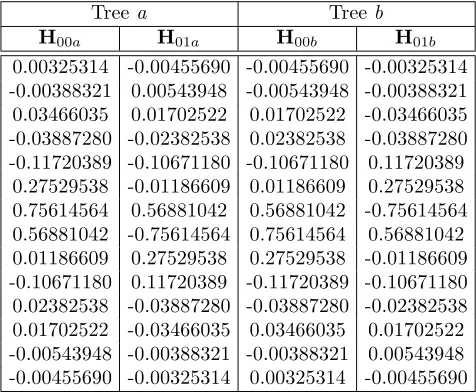
The table of coefficients of the analysing filters in the first stage and the remaining levels are shown in Table 1 and Table 2, respectively. The filters are chosen from [11] by considering shift invariance and directional selectivity at the same time. The coefficients of the synthesis filters are simply the transposes of the analysis filters (orthogonal filters). However, in this paper, we only use texture features extracted from DT CWT subbands which are resulted fromS-level DT CWT decomposition of an input image. The impulse responses of the six complex wavelets associated with the analysis filters given in Table 1 and Table 2 are illustrated in Figure 2 are shown in Figure 2. As can be noticed from Figure 2, there are six subbands characterising features along lines at angles ofθ={±15◦,±45◦,±75◦}. On the other hand, the equivalent 3
[image:5.595.93.505.110.270.2]Table 1: First level coefficients of the analysis filters.
Treea Treeb
H0a H1a H0b H1b
0.02674876 0.04563588 0.02674876 0.04563588 -0.01686412 -0.02877176 -0.01686412 -0.02877176 -0.07822327 -0.29563588 -0.07822327 -0.29563588 0.26686412 0.55754353 0.26686412 0.55754353 0.60294902 -0.29563588 0.60294902 -0.29563588 0.26686412 -0.02877176 0.26686412 -0.02877176 -0.07822327 0.04563588 -0.07822327 0.04563588 -0.01686412 0 -0.01686412 0
0.02674876 0 0.02674876 0
Table 2: Remaining levels coefficients of the analysis filters.
Treea Treeb
H00a H01a H00b H01b
0.00325314 -0.00455690 -0.00455690 -0.00325314 -0.00388321 0.00543948 -0.00543948 -0.00388321 0.03466035 0.01702522 0.01702522 -0.03466035 -0.03887280 -0.02382538 0.02382538 -0.03887280 -0.11720389 -0.10671180 -0.10671180 0.11720389
0.27529538 -0.01186609 0.01186609 0.27529538 0.75614564 0.56881042 0.56881042 -0.75614564 0.56881042 -0.75614564 0.75614564 0.56881042 0.01186609 0.27529538 0.27529538 -0.01186609 -0.10671180 0.11720389 -0.11720389 -0.10671180 0.02382538 -0.03887280 -0.03887280 -0.02382538 0.01702522 -0.03466035 0.03466035 0.01702522 -0.00543948 -0.00388321 -0.00388321 0.00543948 -0.00455690 -0.00325314 0.00325314 -0.00455690
at 45◦.
The Figure 5 illustrates the decomposition of the texture image both in the DT CWT and the DWT domain. For each decomposition only two levels are shown. From these figures it is clearly evident that the DT CWT can distinguish the direction in many different orientations compared to the DWT.
3. Proposed method for texture classification and retrieval
3.1. Feature extraction
TheS-level DT CWT decomposition of anW×H imageI results in a decimated dyadic decomposition intos= 1,2, . . . , Sscales, where the size of subbands at each scale isW/2s×H/2s. Each decimated scale has
a setCs of 6 subbands of complex coefficients, denoted asCs={α(1s)eiθ
(s)
1 , . . . , α(s)
6 eiθ
(s)
6 } corresponding to
responses of the 6 subbands respectively orientated at−15◦,−45◦,−75◦, 15◦, 45◦, and 75◦. For each subband
orientation at scale s there are two responses: magnitude (α(is)) and phase (θ
(s)
i ) responses,i = 1, . . . ,6.
Each response is a 2-D data of sizeW/2s×H/2s, and normalized as follows:
α(is)= α
(s)
i
Eα(is)
, θ (s)
i =
θ(is) Eθi(s)
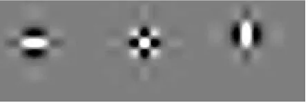
[image:6.595.177.415.294.490.2]Figure 4: The impulse responses of the DWT filters for the 3 directional subbands, all illustrated at level 4 of the transforms. From left to right, 0◦, 45◦, and 90◦subbands.
[image:7.595.79.517.232.359.2](a) (b) (c)
Figure 5: The 2-level decomposition of the (a) original texture image in both, (b) the DWT, and (c) DT CWT domain
where
Eα(is)=
H/2s X
y=1
W/2s X
x=1
α(is)(x, y)2,
Eθi(s)=
H/2s X
y=1
W/2s X
x=1
θi(s)(x, y)2.
Texture features are extracted using image statistics. Unlike in [13] where the variance and entropy are defined in terms of only the magnitude of the DT CWT subbands, in this paper we define a variance
M1(r) and an entropyM2(r) that incorporate both the magnitude and phase responses as the features for
r, r∈ {α(is), θ(is)}, i.e.,
M1(r) =
22s
HW
H/2s X
y=1
W/2s X
x=1
(r(x, y)−µ(r))2,
M2(r) =−
22s
HW
H/2s X
y=1
W/2s X
x=1
r(x, y)2log(r(x, y)2),
where
µ(r) = 2
2s
HW
H/2s X
y=1
W/2s X
x=1
r(x, y).
UsingMk(r),k∈ {1,2}, the following feature vectors are defined for scalesusing the setCs:
FMk,α,s=
h
Mk(α(1s)). . . Mk(α(6s)) i
,
FMk,θ,s= h
Mk(θ(1s)). . . Mk(θ(6s)) i
,
Fα,s=
FM1,α,s
kFM1,α,sk
FM2,α,s
kFM2,α,sk
,
Fθ,s=
F
M1,θ,s
kFM1,θ,sk
FM2,θ,s
kFM2,θ,sk
,
Fs=
F
α,s
kFα,sk
Fθ,s
kFθ,sk
, (2)
wherek.kis the second norm (i.e., the signal energy).
Given an imageI, the multiscale feature vector is extracted by combining different realizations of Eq. 2 for different values of scaless, i.e.;
FIS = [F1 F2 · · · FS]
k[F1 F2 · · · FS]k
(3)
=
fI
S,1fS,I2fS,I3 · · · fS,I24S−2fS,I24S−1fS,I24S
,
whereFIS is a vector of 24S elements.
3.2. Texture learning and classification
Assume that each training set for texture class t consists ofK texture samples. In order to perform a supervised texture classification using DT CWT, the following learning stage for the texture classifier based on that in [13] but modified to include phase information and the newly defined feature vectors for each texture classt:
(i) Decomposekth training texture image I(k)
t using S levels of DT CWT and normalize magnitude and
phase responses of each subband according to Eq. (1). (ii) Generate feature vectorFI
(k) t
S for decomposed texture image.
(iii) Repeat steps (i) and (ii) for all sample images in the same texture class and generate texture feature setFt,S =
FI
(k) t
S
, and store them in the database.
After the features have been learned for each texture class, the following classification stage is performed to classify an unknown imageIu:
(i) Decompose an unknown texture image Iu using S levels of DT CWT and extract its feature vector
FIu
S using Eq. 3.
(ii) Calculate the distance betweenFIu
S and texture feature setFt,S of each classtas
Dt=d
FIu
S ,Ft,S
,
whered( ) is similarity function.
(iii) Assign the unknown texture to texture class iifDi< Dj for alli6=j.
In [13], the similarity function between the query texture and texture class t is simply the normalized Euclidian distance between the feature vectors of the query texture and the mean feature vector of the texture class t. In this paper, the average of the distances between a query feature vector and feature vectors of each sample in each texture class is used, i.e.,
dFIu
S ,Ft,S
= 1 K K X k=1 v u u u t 1 24S 24S X i=1
fIu
S,i−f I(k)
where for texture classt
σt,i =
v u u t
1 (K−1)
K
X
k=1
fI (k) t
S,i −µ
2
where
µ= 1
K
K
X
k=1
fI (k) t
S,i .
3.3. Texture retrieval
Texture retrieval is viewed as a search for the best N, i.e., most similar, images to a given query image
Iq from a database of a totalM images, Im, m= 1,2,· · ·, M. For this purpose, each image is represented
by a feature vector as in Eq. 3. The similarity between two images is measured by the distance between the corresponding feature vectors. The goal is to select among theM possible distances images with theN
smallest distances, in a ranked order, that are most similar toIq.
Given two imagesIq andIm, and letFISq andF Im
S represent the corresponding feature vectors extracted
usingS level DT CWT decomposition according to Eq. 3. We define a distance measure,d(FIq
S,F Im
S ),F Iq
S
andFIm
S as
d(FIq
S,F Im
S ) =
24S
X
i=1 |fIq
S,i−f Im
S,i|
σi (4)
whereσi is defined for the feature vectors of the images in the database, i.e.,
σi =
v u u
t 1
(M−1)
M
X
m=1
fIm
S,i −µi
2
,
and
µi=
1
M
M
X
m=1
fIm
S,i.
4. Experimental results
4.1. Data
The effectiveness of the proposed texture feature extraction approach to texture classification is evaluated by performing supervised classification of several test images with varying texture complexities from two commonly-used natural texture image databases: 128 images from MIT VisTex colour image database [17] and 111 monochrome images from Brodatz Album [18]. Each texture image has a size of 512×512, with 256 grey levels. Each image is globally histogram equalized to ensure that the textures are not trivially discriminable simply based on the local mean or local variance. Different portions of the input patterns of each texture class are selected and used for training the texture classifier. We avoid using the texture patterns on a texture border for training because these patterns are not representative of the texture.
Each texture image is divided into two non-overlapping parts of size 256×512, one for training and one for testing. Overlapped samples are generated from the training texture images using a sliding window of sizeK×K (K = 128) which is moved with shifts of ∆ in both the horizontal and vertical directions. The number of test samples varies with the value of ∆. The value of ∆ is set to 24 to give a reasonable overlap between two test samples, thus a total of 128 texture samples are used in training for each class. After training, another 128 samples for each class are used to evaluate the performance of the texture classifier. Thus, for MIT VisTex database, tests are carried out on 128×128 = 16384 sample images.
In texture retrieval tests, MIT VisTex database and Brodatz Album are used together. Each texture image is uniformly sampled with 8 non-overlapping sub-images of size 128×128, and thus a database of size 239×16 = 3824 is constructed. The query image is searched in this large database, and the top matches for the query image are used in performance evaluations.
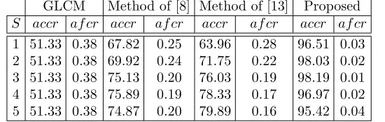
Table 3: Performance results (in %) of different methods for different number of scaleSon MIT VisTex texture database.
GLCM Method of [8] Method of [13] Proposed
S accr af cr accr af cr accr af cr accr af cr
1 51.33 0.38 67.82 0.25 63.96 0.28 96.51 0.03 2 51.33 0.38 69.92 0.24 71.75 0.22 98.03 0.02 3 51.33 0.38 75.13 0.20 76.03 0.19 98.19 0.01 4 51.33 0.38 75.89 0.19 78.33 0.17 96.97 0.02 5 51.33 0.38 74.87 0.20 79.89 0.16 95.42 0.04
4.2. Performance evaluation metrics
The performance of a texture classifier is measured using a confusion matrixCM[19]. CMis aL×L
matrix forLdifferent texture classes andCM(i, j) refers to the classification rate when samples from classi
are identified as classj. Two figure of merits are used in conjunction withCM: average correct classification rate (accr) and average false classification rate (af cr), where
accr= 1
L
X
∀(i,j),i=j
CM(i, j), (5)
af cr= 1
L×(L−1)
X
∀(i,j),i6=j
CM(i, j). (6)
In the experiments for texture retrieval, a query image is any one of the 3824 images in our database. The relevant images for each query are defined as the other 15 subimages from the same image in our texture database. Following [20], we evaluated the performance of the proposed system in terms of the average rate of retrieving relevant images as a function of the number of best retrieved images given a distance measure
dused for comparing feature vectors, i.e.,
RTi =
1
N
N
X
k=1
PT(ki)
N(k), (7)
where RTi is the average retrieval rate of the database when the best Ti images are retrieved from the
database,PT i(k)is the number of correctly retrieved images among theTi retrieved images whenkthimage is
the query image, andN(k)is the total number of relevant images tokthquery images. For texture retrieval
database used in this work,N= 3824, andN(k)= (16−1) = 15.
4.3. Evaluation of texture classification capability
In the experiments for texture classification, in addition to the proposed method, the methods in [13] and [8] are implemented. For [13], we employed the same analysis filters as shown in Table 1 and Table 2. Meanwhile, for [8] we use Daubechies eight tap wavelet low-pass and high pass-filter coefficients respectively as suggested in [8]. It is worth to mention that the method of [8] employ DWT and rotated wavelet transform (RWT) to decompose an input image into 6 directional subbands at each level of decomposition to improve directional selectivity. We also implemented the Haralick texture classification method [21] based on grey-level co-occurrence matrix (GLCM). Only a subset of the 14 Haralick features (i.e., energy, contrast, correlation, entropy, homogeneity, cluster shade and cluster prominence) representing the most commonly chosen ones are used in our study. More details on the extraction of Haralick features can be found in [21].
4.3.1. Comparisons and effect of number of scales
1 2 3 4 5 50
55 60 65 70 75 80 85 90 95 100
S
accr(%)
GLCM Kokare et al. Celik & Tjahjadi Proposed
1 2 3 4 5
0 0.05 0.1 0.15 0.2 0.25 0.3 0.35 0.4
S
afcr(%)
(a)
1 2 3 4 5
60 65 70 75 80 85 90 95 100
S
accr(%)
GLCM Kokare et al. Celik & Tjahjadi Proposed
1 2 3 4 5
0 0.05 0.1 0.15 0.2 0.25 0.3 0.35 0.4
S
afcr(%)
[image:11.595.77.521.167.362.2](b)
Figure 6: Performance comparisons (in %) of different methods for different number of scalesSon different texture databases: (a) MIT VisTex database; and (b) Brodatz Album.
(a) (b) (c) (d)
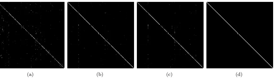
Figure 7: Confusion matrices with maximum correct classification rate of different methods resulted from classification tests on MIT VisTex texture database: (a) GLCM; (b) Method of [8] whenS= 4; (c) Method of [13] whenS= 5; and (d) Proposed method whenS= 3.
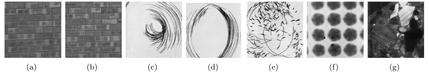
[image:11.595.82.519.511.637.2](a) (b) (c) (d) (e) (f) (g)
Figure 8: Texture samples from MIT VisTex and Brodatz Album texture databases: (a) Brick.0000; (b) Brick.0001; (c) D43; (d) D44; (e) D45; (f) D48; and (g) D59.
the purpose of presentation its performance is also tabulated for each value of scale parameterS. It is clear from test results that the performance of GLCM is the worst. This is mainly due to the co-occurrence matrices derived from the images in MIT VisTex texture database do not result in discriminative features for texture classification. The performances of the methods in [8] and [13] are similar. The method in [8] employs statistical features extracted from both DWT and RWT to achieve better directional selectivity with respect to only DWT. For each level of texture decomposition, features are extracted from subbands of both DWT and RWT. Thus, at each level of decomposition, similar to [13], the feature vectors are ex-tracted from 6 subbands, which are equally distributed between 0-90 degree directions. Since, the direction representation in DT-CWT transform is better than DWT+RWT, the texture classification performance of the method in [13] is better than the method in [8] whenS >1. However, when single-level of wavelet decomposition is considered, i.e.,S= 1, the performance of [8] is better than that of [13]. This is due to the reason that the wavelet filters employed in [13] is longer in length than that of [8] which results in better directional selectivity when S >1. It is clear that the proposed classifier outperforms the other classifiers considered in this paper for different values ofS. That is, when the maximum performances are considered, the proposed method achieves 46.86%, 22.30%, and 18.30% improvements with respect to GLCM, [8], and [13], respectively. The maximum performance is achieved whenS= 3 where the proposed classifier achieves
accr of 98.19% and af cr of 0.01%. The performance of the proposed classifier shows degradations when
S >3. This is mainly due to insufficient number of data points whenS >3 to extract discriminative features for the feature vector. The improvement with respect to [13] is due to the design of texture classifier and consideration of texture features extracted from phase information.
The confusion matrices with maximum correct classification rate of different methods are shown as an image in Figure 7. The confusion matrices as shown in Figure 7 are realizations when maximum correct classification rate is achieved, i.e., S = 4 for [8], S = 5 for [13], and S = 3 for proposed method. In Figure 7 a white square corresponds to 1, a black square corresponds to 0, and values in between 0 and 1 are denoted by squares of varying grey shades. Thus, the more white squares there are in the diagonal of an confusion matrix image, the better is the performance of the corresponding method. It is clear from the confusion matrices as shown in Figure 7 that the proposed method achieves very high classification rate and almost diagonal confusion matrix. When the Figure 7 is observed closely, the diagonal element with index 62 (Food.0009) is classified as 61 (Food.0008). This is due to the reason that both images in original MIT VisTex texture database are the same. The lowest accrof 88.28% is realized for texture Brick.0000. Brick.0000 is classified as Brick.0001 with 11.72% of times. Meanwhile, for Brick.0001, the classifier achieves
accr= 91.40%, and Brick.0001 is classified as Brick.0000 with 8.60% of times. The corresponding textures as shown in Figure 8(a) and 8(b) are very similar in pattern and hard to discriminate.
Table 4: Performance results (in %) of different methods for different number of scaleSon Brodatz Album texture database.
GLCM Method of [8] Method of [13] Proposed
S accr af cr accr af cr accr af cr accr af cr
1 60.75 0.36 69.15 0.28 72.72 0.25 95.63 0.04 2 60.75 0.36 77.36 0.21 80.75 0.17 98.21 0.02 3 60.75 0.36 82.55 0.16 86.18 0.13 98.52 0.01 4 60.75 0.36 80.32 0.18 86.88 0.12 96.39 0.03 5 60.75 0.36 78.82 0.19 86.88 0.12 94.48 0.05
(a) (b) (c) (d)
Figure 9: Confusion matrices with maximum correct classification rate of different methods resulted from classification tests on Brodatz Album texture database: (a) GLCM; (b) Method of [8] whenS= 3; (c) Method of [13] whenS= 4; and (d) Proposed method whenS= 3.
other classifiers considered in this paper for different values ofS. That is, when the maximum performances are considered, the proposed method achieves 37.77%, 15.97%, and 11.64% performance improvements with respect to GLCM, [8], and [13], respectively. The maximum performance is achieved whenS = 3 where the proposed classifier achievesaccrof 98.52% andaf crof 0.01%.
[image:13.595.139.453.590.731.2]The confusion matrices with maximum correct classification rate of different methods are shown as an image in Figure 9. The confusion matrices as shown in Figure 9 are realizations when maximum correct classification rate is achieved, i.e.,S = 3 for [8],S= 4 for [13], andS= 3 for proposed method. It is clear from confusion matrices as shown in Figure 9 that the proposed method achieves almost diagonal confusion matrix. The lowestaccr of 69.53% is realized for texture D43. The very next lowest value is 82.81%. The confusion matrix of texture class D43 created from the confusion matrix as shown in Figure 9(d) according to non-zero entries D43 row is shown in Table 5. According to this matrix, one can say that the texture class
Table 5: The confusion matrix of texture class D43 from Brodatz Album created from confusion matrix of the proposed method as shown in Figure 9(d) according to non-zero entries of row corresponding to D43.
.
D15 D18 D43 D44 D45 D59 D72 D88 D89 D96 D15 100.00 0.00 0.00 0.00 0.00 0.00 0.00 0.00 0.00 0.00 D18 0.00 100.00 0.00 0.00 0.00 0.00 0.00 0.00 0.00 0.00 D43 0.78 0.78 69.53 14.84 5.47 1.56 2.34 0.78 2.34 1.56 D44 0.00 0.00 6.25 91.41 1.56 0.00 0.00 0.00 0.00 0.00 D45 0.00 0.00 2.34 0.00 91.41 0.00 0.00 1.56 0.00 0.78 D59 0.00 0.00 0.00 0.00 0.00 95.31 0.00 0.00 0.00 0.00 D72 0.00 0.00 0.00 0.00 0.00 0.00 92.97 0.00 0.00 0.00 D88 0.00 0.00 0.00 0.00 0.00 0.00 0.00 92.97 0.78 0.00 D89 0.00 0.00 0.00 0.00 0.00 0.00 0.00 0.00 98.44 0.00 D96 0.00 0.00 0.00 0.00 0.00 0.00 0.00 0.00 0.00 100.00
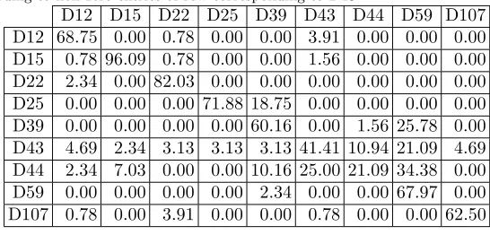
Table 6: The confusion matrix of texture class D43 from Brodatz Album created from confusion matrix of GLCM method as shown in Figure 9(a) according to non-zero entries of row corresponding to D43.
.
[image:14.595.175.421.304.416.2]D12 D15 D22 D25 D39 D43 D44 D59 D107 D12 68.75 0.00 0.78 0.00 0.00 3.91 0.00 0.00 0.00 D15 0.78 96.09 0.78 0.00 0.00 1.56 0.00 0.00 0.00 D22 2.34 0.00 82.03 0.00 0.00 0.00 0.00 0.00 0.00 D25 0.00 0.00 0.00 71.88 18.75 0.00 0.00 0.00 0.00 D39 0.00 0.00 0.00 0.00 60.16 0.00 1.56 25.78 0.00 D43 4.69 2.34 3.13 3.13 3.13 41.41 10.94 21.09 4.69 D44 2.34 7.03 0.00 0.00 10.16 25.00 21.09 34.38 0.00 D59 0.00 0.00 0.00 0.00 2.34 0.00 0.00 67.97 0.00 D107 0.78 0.00 3.91 0.00 0.00 0.78 0.00 0.00 62.50
Table 7: The confusion matrix of texture class D43 from Brodatz Album created from confusion matrix of method in [8] as shown in Figure 9(b) according to non-zero entries of row corresponding to D43.
.
D25 D43 D44 D48 D59 D91 D107 D108 D25 92.97 0.00 0.00 0.00 0.78 0.00 0.00 0.00 D43 0.78 56.25 17.19 15.63 3.13 3.13 3.13 0.78 D44 0.00 17.97 50.00 29.69 0.00 0.00 0.00 0.00 D48 0.00 0.00 0.00 99.22 0.78 0.00 0.00 0.00 D59 0.00 0.00 0.00 9.38 71.09 0.78 0.00 0.00 D91 0.00 0.00 0.00 7.81 13.28 62.50 0.00 0.00 D107 0.00 0.00 0.00 0.00 0.00 0.00 85.94 9.38 D108 0.00 4.69 0.00 0.00 0.00 0.00 14.84 58.59
D43 is mainly misclassified as D44 and D45. The corresponding texture images are shown in Figure 8. When texture images of size 128×128 are cropped from these images, it is highly possible that those images might sample regions with uniform grey-level without any texture on them. Because of this reason, the proposed method has performance degradation on this texture. However, when the context of texture images are observed, one can say they have similar pattern, e.g., circular patterns. Similarly, the confusion matrices of texture D43 for GLCM method, method of [8], and method of [13] are given in Table 6, Table 7, and Table 8, respectively. The GLCM method mainly misclassifies the texture D43 into D44 and D59. Meanwhile, the methods of [8] and [13] perform similarly, and mainly misclassify D43 as D44 and D48. The texture images D48 and D59 are also shown in Figure 8. However, when the image patterns of D48 and D49 are closely observed, one can say that the resemblance to D43 is not high. This also shows that the proposed method makes better classification in terms of contextual information embedded in texture images.
As can be observed from Table 3 and Table 4, the performance of the proposed multiscale classifier depends on the number of scalesS used in feature extraction. The proposed algorithm performs well for
S = 3 on 128×128 test images. However, when the image size gets larger, it might be necessary to use higher values of S to achieve high classification performance. Meanwhile, for the smaller size of images, the lower values of S should be selected. Thus the performance of the proposed method can be further improved when the number of scales are automatically estimated by considering the size and content of the input image.
4.3.2. The effect of the number of samples used in training
Figure 10 and Table 9 show the performance results of the proposed method for different values ofK
Table 8: The confusion matrix of texture class D43 from Brodatz Album created from confusion matrix of method in [13] as shown in Figure 9(c) according to non-zero entries of row corresponding to D43.
.
D25 D43 D44 D45 D48 D59 D91 D107 D25 92.97 0.00 0.00 0.00 0.00 0.00 0.00 0.00 D43 1.56 54.69 17.97 0.78 14.84 2.34 3.91 3.91 D44 0.00 25.00 42.97 0.00 28.13 3.13 0.78 0.00 D45 0.00 74.22 0.00 18.75 0.00 0.00 0.00 0.00 D48 0.00 0.00 0.00 0.00 98.44 0.00 1.56 0.00 D59 0.00 0.00 0.00 0.00 9.38 60.16 10.94 0.00 D91 0.00 0.00 0.00 0.00 9.38 6.25 70.31 0.00 D107 0.00 0.00 0.00 0.00 0.00 0.00 0.00 93.75
0 50 100 150
55 60 65 70 75 80 85 90 95 100 K accr(%)
0 50 100 150
0 0.05 0.1 0.15 0.2 0.25 0.3 0.35 K afcr(%) (a)
0 50 100 150
65 70 75 80 85 90 95 100 K accr(%)
0 50 100 150
0 0.05 0.1 0.15 0.2 0.25 0.3 0.35 K afcr(%) (b)
Figure 10: The texture classification performance of the proposed method on MIT VisTex and Brodatz Album texture databases for different number of texture samplesKused in training stage whenS=3: (a) Results on MIT VisTex texture database; and (b) Results on Brodatz Album texture database.
method and almost the same with the methods of [8] and [13] when they are trained using full training set of 128 texture images per texture class. This makes the proposed method useful for texture classification applications where the number of texture samples used in training is limited. Ignoring very small fluctuations on the performance curves in Figure 10, the performance of the proposed classifier stabilises whenK >8.
4.4. Evaluation of texture retrieval capability
The effectiveness of an image retrieval system is measured using a average retrieval rate graph. In constructing such a graph, the top matching Ti texture images for a query texture image are retrieved
from a database, and for each retrieval, the average retrieval rate is calculated according to Eqn. (7). It is empirically found that for the database constructed for texture retrieval experiments, the other methods, [8] and [13], perform the best whenS= 5 is used in wavelet decomposition. Thus, comparisons are presented forS= 5.
The texture retrieval performances of different methods are shown in Figure 11 and tabulated in Table 10. Similar to the texture classification, GLCM achieves the worst performance in texture retrieval. This is mainly because the database consists of many texture samples with similar grey-level distributions but different shapes. The texture retrieval performance is significantly increased by employing wavelet transform techniques which rely on the high frequency components (edges) of texture images at different resolutions. The performances of the methods in [8] and [13] are almost the same. This is mainly because both methods
Table 9: The texture classification performance results of the proposed method on MIT VisTex and Brodatz Album texture databases for different number of texture samplesKused in training stage whenS=3.
MIT VisTex Brodatz Album
K accr af cr accr af cr
1 56.77 0.34 68.42 0.29 2 66.64 0.26 75.36 0.22 4 75.72 0.19 81.64 0.17 8 83.55 0.13 86.91 0.12 16 89.61 0.08 91.22 0.08 32 93.98 0.05 94.49 0.05 64 96.80 0.03 97.22 0.03 128 98.19 0.01 98.52 0.01
20 40 60 80 100 120 140 160 180 200
50 55 60 65 70 75 80 85 90 95 100
Number of retrieved images considered
Average retrieval rate (%)
GLCM Kokare et al. Celik & Tjahjadi Proposed
Figure 11: Texture retrieval performances (in %) of different methods according to the average retrieval rate (RTi) given in Eqn. (7) whereS= 5 is used for all methods except GLCM method.
use almost the same directionality at each resolution. By using the phase together with the magnitude information increases the texture retrieval capacity of the proposed method when compared with the methods in [8] and [13], thus achieving the best performance.
Qualitative evaluation of the proposed method is carried out by visually examining the images of retrieval results. However, this can only be based on a subjective perceptual similarity since there exists no “correct” ordering that is agreed upon by all people. In Figure 12, some examples of retrieval results from the proposed are shown. In Figure 12(a), the query image is Fabric.0013 from MIT VisTex texture database. The system almost perfectly retrieves all images of the same fabric and also images of other types of fabrics. When images are carefully observed, one can say that the retrieved texture images are almost the same type. In Figure 12(b), the query is texture D27 from Brodatz album. In this case, all relevant images except one are correctly ranked as the top matches following by images of similar textures. The texture image Food.0006 as shown in Figure 12(c) does not have a certain texture pattern. However, the proposed method can still make a perfect match according to the top three best matches from the database. The rest of retrieved images somehow related to the query image. Figure 12(c), the query D77 texture image from Brodatz Album. In this case, all relevant images are correctly ranked as the top matches following by images of similar textures. The rest of four matches are similar to the query texture pattern.
The value of S affects the texture retrieval capacity of the proposed method. Figure 13 shows the performance of the proposed texture retrieval algorithm in terms of RTi for different number of scales S.
Table 10: Texture retrieval performance results (in %) of different methods according to the average retrieval rate (RTi) given in Eqn. (7) whereS= 5 is used for all methods except GLCM method.
GLCM Method of [8] Method of [13] Proposed
Ti RTi (in %) RTi (in %) RTi (in %) RTi (in %)
15 51.12 66.88 72.32 74.22
20 56.40 73.44 78.64 81.24
40 66.27 83.13 86.96 90.24
60 71.07 87.30 90.24 93.62
80 74.43 89.82 92.32 95.71
100 77.06 91.69 93.79 96.99
120 79.06 93.09 94.84 97.98
140 80.76 94.21 95.75 98.74
160 82.21 95.10 96.49 99.37
180 83.50 95.85 97.04 99.94
200 84.67 96.52 97.55 100.00
(a) (b) (c) (d)
Figure 12: Examples of retrieval results from 3824 texture images. The query image is at the top left corner of each group of images, and the other images are ranked in the order of similarity with the query image from top left plus 1 to bottom right. The query images are a subimage of: (a) Fabric.0013; (b) D27; (c) Food.0006; and (d) D77.
20 40 60 80 100 120 140 160 180 200
60 65 70 75 80 85 90 95 100
Number of retrieved images considered
Average retrieval rate (%)
S=1 S=2 S=3 S=4 S=5
[image:17.595.187.407.498.688.2](a)
Figure 13: Texture retrieval performances (in %) of the proposed method according to the average retrieval rate (RTi) given in Eqn. (7) under different scale parametersS.
expense of higher computational cost.
5. Conclusion
In this paper, we proposed a new texture classifier structure which uses both the magnitude and phase of DT CWT subbands. The coarse approximation of the signal is not used for feature extraction since it is more prone to illumination changes. For each texture image, a multiscale texture feature vector is extracted from the magnitude and phase of DT-CWT subbands at different scales.
It is empirically shown that for texture classification the proposed classifier outperforms recently proposed texture classifiers. It achieves 98.19% and 98.52% correct classification rates in whole MIT VisTex and Brodatz Album texture databases, respectively. It is also shown that the use of phase information together with the magnitude information improves the performance significantly.
The proposed method can achieve a high texture classification rate even for small number of samples used in training stage. This makes it suitable for applications where the number of texture samples used in training is very limited.
It is shown that for texture retrieval the proposed texture retrieval algorithm outperforms recently proposed texture retrieval algorithms. The average retrieval rate of the proposed texture retrieval algorithm increases when the number of the scalesS is increased. However, the increase in performance is achieved at the expense of an increase in computational load.
Acknowledgments
The authors would like to thank Warwick University Vice Chancellor Scholarship for providing the funds for this research.
References
References
[1] O. Faugeras, Texture analysis and classification using a human visual model, in: Proceedings of IEEE International Conference on Pattern Recognition, 1978, pp. 549–552.
[2] A. Jain, F. Farrokhnia, Unsupervised texture segmentation using gabor filters, Pattern Recognition 24 (12) (1991) 1167– 1186.
[3] S. Arivazhagan, L. Ganesan, S. Priyal, Texture classification using gabor wavelets based rotation invariant features, Pattern Recognition Letters 27 (16) (2006) 1976–1982.
[4] S. Arivazhagan, L. Ganesan, Texture classification using wavelet transform, Pattern Recognition Letters 24 (2003) 1513– 1521.
[5] S. Arivazhagan, L. Ganesan, Texture segmentation using wavelet transform, Pattern Recognition Letters 24 (2003) 3197– 3203.
[6] K. Muneeswarana, L. Ganesanb, S. Arumugamc, K. Soundara, Texture classification with combined rotation and scale invariant wavelet features, Pattern Recognition 38 (2005) 1495–1506.
[7] S. Kim, T. Kang, Texture classification and segmentation usingwavelet packet frame and gaussian mixture model, Pattern Recognition 40 (2007) 1207–1221.
[8] M. Kokare, P. Biswas, B. Chatterji, Texture image retrieval using rotated wavelet filters, Pattern Recognition Letters 28 (2007) 1240–1249.
[9] P. Hiremath, S. Shivashankar, Wavelet based co-occurrence histogram features for texture classification with an application to script identification in a document image, Pattern Recognition Letters 29 (2008) 1182–1189.
[10] M. Do, M. Vetterli, Wavelet-based texture retrieval using generalized gaussian density and kullback-leibler distance, IEEE Transactions on Image Processing 11 (2) (2002) 146–158.
[11] N. Kingsbury, Complex wavelets for shift invariant analysis and filtering of signals, Applied and Computational Harmonic Analysis 10 (3) (2001) 234–253.
[12] S. Hatipoglu, S. Mitra, N. Kingsbury, Texture classification using dual-tree complex wavelet transform, in: International Conference on Image Processing And Its Applications, 1999, pp. 344–347.
[13] T. Celik, T. Tjahjadi, Multiscale texture classification using dual-tree complex wavelet transform, Pattern Recognition Letters 30 (3) (2009) 331–339.
[15] A. Vo, S. Oraintara, A study of relative phase in complex wavelet domain: Property, statistics and applications in texture image retrieval and segmentation, Signal Processing: Image Communication 25 (1) (2010) 28–46.
[16] Y.-L. Qiao, C.-H. Zhao, C.-Y. Song, Complex wavelet based texture classification, Neurocomputing 72 (16-18) (2009) 3957–3963.
[17] MITVisTex, Vision texture database,http://www.media.mit.edu/vismod/(1998).
[18] P. Brodatz, Textures: A Photographic Album for Artists and Designers, Dover, New York, USA, 1966. [19] R. Kohavi, F. Provost, Glossary of Terms, Vol. 30, Kluwer Academic Publishers, Hingham, MA, USA, 1998.
[20] B. Manjunath, W. Ma, Texture features for browsing and retrieval of image data, IEEE Transactions on Pattern Analysis and Machine Intelligence 18 (8) (1996) 837–842.
[21] R. M. Haralick, K. Shanmugam, I. Dinstein, Textural features for image classification, IEEE Trans. Sys. Man Cybern. 3 (6) (1973) 610–621.
Turgay C¸ elikreceived the Ph.D. degree in engineering from the University of Warwick, U.K., in 2011. He has produced extensive publications in various international journals and conferences. He has been acting as a reviewer for various international journals and conferences. His research interests are in the areas of biophysics, digital signal, image and video processing, pattern recognition and artificial intelligence, unusual event detection, remote sensing, and global optimization techniques.
Tardi Tjahjadi(SM’02) received the B.Sc. (Hons.) degree in mechanical engineering from University

![Table 8: The confusion matrix of texture class D43 from Brodatz Album created from confusion matrix of method in [13] asshown in Figure 9(c) according to non-zero entries of row corresponding to D43.](https://thumb-us.123doks.com/thumbv2/123dok_us/9672944.469114/15.595.75.520.137.455/confusion-texture-brodatz-confusion-figure-according-entries-corresponding.webp)
