Aggression Based Audio Ranking : Annotation and Automatic Ranking

(1)

1

Faculty of Electrical Engineering,

Mathematics & Computer Science

Aggression Based Audio Ranking

Annotation and Automatic Ranking

Daan H. Wiltenburg M.Sc. Thesis

August 2019

Supervisors:

(2)

(3)

Summary

In many places, public and private, aggression can be a big problem. Therefore, surveillance is essential. Sound Intelligence builds software especially for this purpose. Currently an aggression classifier is used as surveillance assistant. In this study, techniques from the field of information retrieval are applied in order to improve the performance of this classifier. More specifically, aggression based audio ranking is investigated.

To automatically rank audio files, a ground truth is needed. Therefore this research is twofold. The first part of this research focuses on annotation of the data set. Different methods of rank annotations are compared on transitivity and efficiency. The annotation methods are based on pairwise and list-wise comparisons. The methods are compared on time efficiency and transitivity. 50 subjects participated in this experiment. First a ground truth is established by pairwise comparing every sample in a subset of the data. This subset is used to evaluate different, more efficient methods. Furthermore, a simulation is done to predict the time needed to annotate a bigger data set.

The results show that a pairwise comparison method based on binary insertion sort is the most efficient way to annotate audio samples into a ranking. To annotate a set of 300 audio samples, this method would take 8 hours whereas the second best method would take 21 hours. Furthermore this method yields the most transitive ranking, with an in-transitivity value of 0.146 which is better than the baseline(0.15) and the list-wise methods(0.157 and 0.169). The pairwise method is used to annotate 300 audio samples into a ranking. The rankings of 4 annotators are used to assemble a data set that is used for supervised machine learning.

The second problem addressed in this research is in the field of machine learning and learning-to-rank. Two type of loss functions are compared. The first loss function is Mean Squared Error, which uses a continuous target between 0 and 1 to train a network making this a regression approach. The second loss function is the log-likelihood function, which takes an ordered list as target making this a list-wise approach. For both approaches two network architectures are developed and optimized: A fully connected neural network and a convolutional neural network. For optimization hyperopt1_{is used. The combination of these}

architectures and loss functions yields 4 models.

The models are evaluated based on the final ranking they yield. The measures used are Kendalls Rank Correlation Coefficient, Spearmans Rank Correlation Coefficient and Mean

1_{Hyperopt is a python library that can be used to perform hyper-parameter optimization.}

(4)

IV SUMMARY

Squared Error. The best model achieved an KRCC of 0.6049, an SRCC of 0.8228 and an MSE of 0.0364. Furthermore, the results are compared to the performance of the anno-tators. This comparison shows that the models yield rankings that correlate moderate to strong with the rankings of annotators.

(5)

Introduction

Although Speech Emotion Recognition(SER) already in the fifties, lately there is a growing interest in this research field. In 2017 more than 150 papers have been published in SER [1]. This review summarizes different classification techniques used in emotion recognition. All techniques described in this paper focus on discreet classification into different emotion labels. Nassif et al. [2] describe supervised machine learning in SER application. They define classification and regression as the main categories of machine learning. Another field in supervised machine learning is learning-to-rank, in which a model predicts a ranking rather than a label or continuous value, is relatively unexplored in SER.

1.1 Sound Intelligence

Sound Intelligence (SI) is a company that uses supervised machine learning techniques for event detection in audio. One of the events that the software of SI can detect is aggression. Currently the software works as a classifier, where some event is either aggression or it is not. The user of the system can modify the sensitivity of the classifier, which determines the trade off between false positives and false negatives. SI wants to extend this software to a more advanced sensitivity system, where this functionality is not a trade of between two wrongs. The new functionality should allow the user to set a threshold from which aggressive events should be reported. This research is aimed to find ways of automatically ranking audio files based on aggression. This ranking will make it possible to set such a threshold, which is a more sophisticated method of control than the current sensitivity control and should lead to fewer false or missed reports.

1.2 Goal of the Research

Supervised machine learning is a specific type of machine learning where the correct output given an input is known [3]. To apply supervised machine learning techniques a labeled data set is needed. The labeling of this data is referred to as data annotation. A set of 2427 unlabeled audio samples is available at SI for this research.

(10)

2 CHAPTER1. INTRODUCTION

The goals of this research are two-fold: First, the different possibilities of data annotation will be investigated in order to determine an efficient way to rank the data set. This data set will be used as a training-, validation and test set for different supervised machine learning techniques.

Secondly, different supervised machine learning techniques are investigated to deter-mine how to automatically rank audio based on aggression.

1.3 Reader’s Guide

(11)

Chapter 2

Background

2.1 Background in Data Annotation for Audio

Susini et al. [4] describe different measurements that are used in psychoacoustics, a field in which ..research aims to establish quantitative relationships between the physical properties of a sound [..] and the perceived properties of the sound [4]. First the classical evaluations methods are described, divided into indirect and direct methods:

• Ratio scaling: In this scenario the sensation related to a sound has to be expressed

on a numerical judgment scale.

• Cross Modal Matching: According to the dictionary of psychology this is A scaling

method [..] in which a [participant] makes the apparent intensity of stimuli across two sensory modalities, as when an [participant] adjusts the brightness of a light to indicate the loudness of [an audio sample]. [5]

Previous methods are usable for stationary sounds, but everyday sounds are not station-ary, neither is aggression. Non stationary sounds require continuous rating of sound. The paper describes five categories of continuous sound judgment:

• Method of continuous judgment using categories: Participants judge an attribute of a

sound in real time into categories ranging from very loud to not loud at all, they change to another category when their evaluation of the sound changes.

• Audiovisual adjustment method: Participants adjust the length of a line proportional to

the auditory sensation in real time.

• Continuous cross-modal matching: this is similar to cross modal matching of a

station-ary sound; only now the participant changes the evaluation modality along the length of the stimulus.

• Analog categorical scaling: Participants can slide a cursor continuously along five

discrete categories [4]. As opposed to continuous judgment using categories, the results are now measured on an analog instead of a discrete scale.

(12)

4 CHAPTER2. BACKGROUND

• Semantic scale used in real time: This is used to track real-time emotional response

to music or sound. In this set up a participant has to evaluate the related sensation on one or more emotion scales in real time when a sound sample is presented.

Next to classical evaluation methods, multi-dimensional and exploratory methods are de-scribed.

• Semantic differential (SD): The participant has to rate stimuli on a semantic scale with

two opposed descriptors. Examples of these descriptors are good-bad or pure-rich. When using SD the participant has to evaluate one stimulus at a time.

• Dissimilarity judgments: Contrary to SD no descriptors are used; now two samples

are compared with each other and rated on similarity scales. Euclidean distance is calculated to determine similarity. This leads toN(N −1)/2comparisons.

• Sorting tasks: listeners are required to sort a set of sounds and to group them into

classes. [4]

• Free sorting tasks: no predefined (number of) classes. Various methods of free sorting

and grouping of stimuli into different categories are explained. Free sorting is out of the scope of this research, for more information the reader should review [4].

• 2AFC: two alternatives, forced choice. Two stimuli are presented, the listener has to

choose one of the two as the best option related to a certain scale (i.e. choose the most aggressive sample).

Following the paper of Susine et al. [4], some interesting categories of sound annotation methods can be defined. These techniques are tested in other papers as well.

2.1.1 Individual Annotation

This is the technique where one stimulus is judged at a time. Continuous sound judgment and SD are techniques described by Susini et al. [4] that fall into this category. A widely used measure for individual affect annotation is the valance (positive/negative) and arousal (high/low) two dimensional scale, proposed by James Russell [6] which can be used to describe every emotion. Because the annotator does not have to name a specific emotion, language ambiguity is omitted.

Individual evaluation is the most time efficient way of annotating data. Since there are no comparisons, the amount of annotations needed is equal to the amount of stimuli. however multiple studies [7]–[10] have shown that this evaluation leads to in-transitive1_results.

(13)

2.1. BACKGROUND INDATAANNOTATION FORAUDIO 5

2.1.2 Paired Comparison

Susini et al. [4] describe Dissimilarity judgments and 2AFC, which is a form of paired com-parison. Parizet, Guyader and Nosulenko [8] used pairwise comparison in their experiment to find the sound of a car door closing, that evokes the best quality. The comparison had to be answered by either choosing one sample, or both samples were perceived equal. 40 participants evaluated 12 sounds, resulting in 66 pairwise comparisons(N(N −1)/2. Ifx

is preferred over y, then the preference score px,y = 1. If y is preferred over x, then the

preference scorepx,y = 0. Ifx andy are indifferent,px,y = 0.5. The preference scores are

averaged over the 40 participants. The correlation between the measured and the estimated probability was 0.94, indicating that this is a very accurate way of comparison. The fact that 66 comparisons are needed to evaluate 12 sounds is a major drawback.

Poirson et al. [9] compare the evaluation of 11 diesel engine sounds by experts and naive subjects, where experts are subjects trained in the evaluation of audio samples. The experiment included two panels: an expert panel, consisting of 10 trained subjects; a panel of naive subjects, consisting of 30 students. They found that the evaluations of experts and naive subjects are very similar when it comes to paired comparison. only 5 out of 30 naive subjects are discarded for giving in-transitive results, indicating that naive subjects can be suitable annotators for paired comparison tests. On the other hand they found that naive subjects find it difficult to evaluate individual sound samples on a numeric scale, leading to in-transitive evaluations.

As opposed to Parizet et al. [8], the participants of [9] did not have to compare the entire comparison matrix. To get computable results the subjects had to compare one full row of the matrix and 12 additional comparisons. This leads to10 + 12 = 22comparisons, instead

of(11∗10)/2 = 55comparisons.

As literature shows, comparisons are more discriminant than judgments. On the other hand this is very time consuming. Furthermore, in most of the above papers the author is working with up to 12 stimuli, where as sound Intelligence is looking for a solution to annotate thousands of files. It is not feasible to compare every stimulus with each other. Therefore two methods of inserting new data into a ranked list will be evaluated on efficiency, which are explained in 5.1.

2.1.3 Binary Insertion Sort

There is a variety of sorting algorithms used in computer science, Binary Insertion Sort is such a sorting algorithm that is widely used. In this method an unranked sample xwill be

compared to multiple samples in the ordered list. The comparison will start with comparing the sampley that is in the middle of the ordered list. If x has a higher value thany,x will

be compared to another sample in the ordered list: the sample right in betweeny and the

end of the ordered list. Ifxhas a lower value thany,xwill be compared to the sample right

(14)

samples to compare with, which will be the position where the new sample is added to the ordered list. This can be used to efficiently build a ranking: O(nlogn).

2.2 Background in Audio Processing

Before mathematical operations can be applied to audio, it has to be transformed to a digital format. When the data is transformed from an analog to a digital signal, the data can be processed digitally. Often this digital signal is transformed into a more usable format. ”Signal analysis transforms a signal from one domain to another, for example from the time domain to the frequency domain. By transforming the signal, the intent is to emphasize information in the signal and cast it into a form that is easier to extract” [11]. In most machine learning applications the wave input files are transformed into the frequency domain because this is a representation of the audio input over which machine learning models can efficiently generalize. To transform the data from the time domain to the time-frequency domain the data has to be processed in small frames. To transform these frames into the frequency domain Fast Fourier Transform (FFT) and Discrete Fourier Transform (DFT) are widely used. These techniques are explained in [11].

A type of audio input that is often used in audio classification are Log-Mel-Spectrums. First the audio signal is transformed to the frequency domain. This is done for a short window of the audio signal using Fourier transformation. The energy spectrum is obtained by taking the this transformation squared. The energy obtained by this transformation are transformed to the Mel scale, which is divided into multiple filterbanks. The logarithms of the powers in these filterbanks form the Log-Mel-Spectrums(LMS) [12], [13].

In speech recognition Mel-Frequency Ceptrum Coefficients (MFCC) are widely used. The MFCC of a signal is obtained by taking the spectrum of the LMS. A spectrum of a spectrum is called a ceptrum [14].

El Ayadi et al. [15] describe different features for emotion detection in audio. They de-scribe energy and pitch as main continuous features. They mention MFCC as widely used frequency feature along with Linear Predictor Ceptral Coefficients (LPCC). Lately there have been experiments on raw audio wave input [16].

2.3 Background in Machine Learning

(15)

2.3. BACKGROUND INMACHINELEARNING 7

2.3.1 Support Vector Machines

A Support Vector Machine (SVM) algorithm is an algorithm that finds the hyper plane that separates data points of two classes, with the maximum margin between the two classes. SVM’s are widely used, but since computational expenses become less of a problem new architectures are replacing SVM’s [17].

2.3.2 Neural Networks

Kevin Gurney [18] published a book calledAn Introduction to Neural Networks in which he

describes the basic concept of Neural Networks. This book gives a clear and understandable explanation to readers who are new to this field. A Neural Network (NN) is a combination of simple mathematical operations in order to learn patterns from a set of training data. An NN consists of multiple layers and these layers typically consists of multiple nodes. The nodes in different layers are connected by weights. Each node receives input from multiple other nodes in the previous layer. Within a node the inputs are summed. Whenever this sum exceeds a certain threshold the neuron will generate an output that can be used for classifi-cation. A typical NN will consist of multiple layers: An input layer, which is a representation

of the data. One or more hidden layers in which operations on the input will take place and an output layer. This output layer can be one node in a binary classification problem, but can also consist of multiple nodes. For example in character recognition this layer might contain 26 nodes, one for each character of the alphabet. Furthermore an NN can be used in a

regression task where the network does not output a classification but predicts a value for a certain input.If all the nodes in layerx are connected to all the nodes in layerx+ 1for all

layers, the network is called a fully connected NN. If the network consists of more than one hidden layer, the network is called a Deep Neural Network (DNN).

2.3.3 Convolutional Networks

Sandro Skansi [19] gives a detailed explanation about Convolutional Neural Networks (CNNs) and their mathematical background in his bookAn introduction to Deep Learning. CNNs are

(16)

2.3.4 Recurrent Neural Networks

Skansi [19] also explains the use of Recurrent Neural Networks (RNNs). An RNN is a type of NN that feeds the output of data pointxback into the network when processing data point x+ 1. This way the network has information about previous inputs, giving it some sort of

memory. Next to that, this makes it possible to process data of different sizes without the need to re-size the input data. This is specifically useful in audio processing for two reasons: First of all when processing audio it can be expected to have samples of different sizes. Next to that silence is an important aspect of audio so padding audio samples with zeros, in order to get same sized data inputs, will change the meaning of these audio samples. This can lead to a drop in accuracy. Two commonly used types of recurrent layers are Long-Short Term Memory (LSTM) and Gated Recurrent Units (GRU).

Sak et al. [20] describes the use of LSTMs in a speech recognition task. An LSTM architecture consists of three gates. An input gate determines which parts of the input to this LSTM layer should be kept. A forget gate, which decides what data is not usable and can be omitted. The final gate is an output gate which determines what should be passed on. An LSTM has two outputs. A cell state which, will be passed on to the LSTM layer of the next data input. Next to the cell state it outputs a hidden state which is used for prediction.

Wu and King [21] apply LSTMs as well as GRUs in a speech processing task. They describe GRUs as similar to LSTM architectures only now the forget and input gates are combined into a reset gate, which reduces the amount of operations making GRUs compu-tationally less expensive. In this reset gate, information is only forgotten if something new is inserted in it’s place.

2.4 Audio Processing Using Machine Learning

2.4.1 Deep Learning Audio Event Detection

Lane et al. [22] describe the development of an audio event detection system intended to run on mobile devices: ”Deep Ear: The first mobile audio sensing framework built from coupled DNNs that simultaneously perform common audio sensing tasks” [22]. The system consists of four DNNs, every network performs a specific task: Ambient audio sensing analysis; speaker identification; emotion detection; stress detection. The framework is optimized for mobile devices by taking into account battery cost and use in a variety of environments. One of the research questions discussed in this paper is:Can deep learning assist audio sensing in coping with unconstrained environments?

(17)

2.4. AUDIOPROCESSINGUSINGMACHINELEARNING 9

anger, fear, neutral, sadness or happiness. Speaker Identification can discriminate between 23 speakers.

To train the system both labeled and unlabeled data is used. The unlabeled data is used as background noise for the labeled data as well as to initialize the DNNs. All DNNs consists of the same architecture: 3 hidden layers with 1024 nodes in each layer. ReLU is used in combination with dropout to optimize the networks.

For validation a benchmark experiment is done, in which Deep Ear is compared to four systems with shallow architectures as oppose to the deep architecture in Deep Ear. These four systems each addressed one specific task that relates to one of the DNNs in Deep Ear. The results show a gain in accuracy for all four aspects, ranging from 7.7% to 82.5% for Ambient Scene Analysis to Speaker Identification respectively.

Deep Ear outperforms systems for comparable tasks greatly when these are trained on clean data. When the same benchmark systems are trained on noisy data, their per-formance improves but are still outperformed by Deep Ear. The Ambient Scene Analysis achieves an accuracy of above 80%, Stress and Emotion Detection both approximately 80% and Speaker Identification approximately 50%.The paper proves that using deep learning techniques greatly outperform shallow systems and can better cope with data with noise on different levels, indicating that deep learning can improve audio sensing with unconstrained environments.

2.4.2 Convolutional Neural Networks and Audio

Piczak [23] developed a system using a Convolutional Neural Network (CNN) to classify environmental sounds from three publicly available data sets: ESC-50, ESC-10 and Urban-Sound8K. The performance of the CNN is compared to a baseline system. The baseline system is a Random Forest with MFCC as input.

The proposed system consists two 2 convolutional layers with max pooling, combined with two fully connected layers. The system uses segmented spectrograms with deltas as input. Furthermore the system makes use of dropout and uses ReLU as activation function. ESC-50 consists of 2000 clips(five seconds each) with a total of 50 balanced classes. The baseline model used in this research scored 44% on this data, human participants achieved an accuracy of 81%, the best CNN proposed in this paper reached an accuracy of 64.5%. ESC-10 consists of 400 of these records and a total of 10 classes, the baseline system reached 73% accuracy, human annotators reached 96% accuracy and the proposed system reached approximately 80%. UrbanSound8k consists of 2732 clips of four seconds or shorter, with a total of 10 classes. The baseline system2_{achieved an accuracy of 73.7%,}

the proposed system an accuracy of 73.1%.

Choi et al. [24] describe the comparison of a Convolutional Recurrent Neural Network (CRNN) to three different CNNs. The networks are tested on a music data set to predict the

(18)

top 50 tags in this set, including genres, moods, instruments and era’s. Approximately 215 thousand clips are used. As a metric, Area Under Receiver Operating Characteristics Curve (AUC-ROC) is used, because the clips are multi-label tagged.

The CRNN uses 4 CNN layers, after that follow two RNN layers with Gated Recurrent Units (GRU). The results show that the CRNN outperforms the CNNs on all experimented amounts of parameters, but needs more training time to achieve this. The highest AUC-ROC achieved by the CRNN is 0.86.

2.4.3 Weakly labeled data

Kong et al. [25] propose a Joint Detection Classification Model (JCD), which finds the in-formative and uninin-formative parts of an audio sample and only uses the inin-formative parts to classify the sample. They describe two types of audio annotation: Clip level annotation, where each clip as one or more labels; Event level annotation, where each clip has one or more labels and every label has an occurrence time. The proposed system is based on human analyses of sound, where the writer assumes that humans detect when to attend to a sound. Subsequently humans classify the sound.

The system takes as input data that is annotated at clip level. The JCD algorithm can output labels at event level, leading to an Equal Error Rate (EER) of 16.9% which is lower than the baseline(19%) without the need of event level annotation.

2.4.4 Varying Length Audio Input

Varying length audio samples can lead to problems in Machine Learning. Since silence is part of audio, padding audio samples to a specific length might not be the best solution. [26] describe the use of a convolutional layer on the input. For the use of acoustic scene classification and domestic audio tagging they use the short-time Fourier transform (STFT) of steps of 25ms as one dimension. The amount of steps depends on the length of the sample, which determines the other dimension. The convolutional layer can handle this varying length, as long as the layer is smaller or equal to the least amount of steps occurring in the data set. The pooling layer will be applied on a dynamic pooling window.

Phan et al. [27] describe another shallow CNN architecture which uses a convolutional layer directly on the input. The network consists of three layers, one convolutional layer, one one-max-pooling layer and a Softmax layer. By using convolutional filters directly on the input, inputs can be of different sizes as long as they are longer than the longest filter. The convolutional layer is followed by a one-max-pooling layer, which reduces each filter to the size of one regardless of the input length. The described architecture makes use of four filters, this leads to a vector of length four after the pooling layer.

(19)

2.5. RANKING ANDMACHINELEARNING 11

of noise are selected. The results show a great improvement of performance compared to the state of the art DNNs (76.3% Relative Error Reduction). The best system achieved a mean accuracy of 98.6% over four different noise levels.

2.5 Ranking and Machine Learning

A field in which ranking algorithms are widely used is information retrieval (IR). Thread or result ranking of big data sets are central problems in this field. These techniques can be relevant for Aggression ranking as well.

Jian Jiao [28] describes a system that is used for the ranking of usefulness of online treads based on specific queries. Furthermore he states that the state of the art ranking algorithms can be divided into three categories:

• Pointwise

• Pairwise

• List-wise

these algorithms are very similar to the described annotation schemes for ranking pur-poses.

2.5.1 Pointwise

For every input a (relevance) score is calculated. The inputs are ordered based on these scores, yielding a ranked list. The ground truth is an ordinal score or numeric value. This output can be human annotated or automatically generated based on some mapping. Li et al. [29] propose such a system.

2.5.2 Pairwise

The input of this algorithm is representations of two documents, the output is a binary value indicating the preferred document. as opposed to pointwise this yields a ranking of two documents. On the other hand, all documents have to be compared to each other to get to an ordered list, which can be computationally expensive. Such a system is proposed in [30].

(20)

2.5.3 List-wise

The final ranking of all the documents is used to determine loss of the model. This is state of the art and is competitive with pairwise approaches. Fang et al. [32] propose a recom-mendation system that is validated on two real world data sets. The first data set consists of product reviews, the second data set consists of movie reviews. The system makes use of list-wise learning-to-rank (LTR) instead of the widely used pointwise ranking. To do so they take the cross entropy between the predicted ranking and the full ground truth ranked list as loss function. The proposed system outperforms pointwise as well as pairwise based systems. Furthermore they use similarity measures to validate individual rankings in order to filter out malicious input.

2.6 Loss Functions

In the different Machine Learning Applications a variety of loss functions are used to evaluate the quality of a regression or ranking output. Furthermore the gradient of this loss function is used to update the model during training. The loss functions used in classification are omit-ted in this paper, since those loss functions are not applicable for the algorithms developed in this project.

2.6.1 Loss Functions for Regression

Mean Squared Error Loss (MSE)

The Mean Squared Error Loss is a widely used error function. It is closely related to the Sum of Square Error function. In both cases the difference between predicted (p) and target

(t) is squared. The squares of every input is summed together. When using Mean Squared

Error Loss, this sum is divided byn. This error is sometimes referred to as L2 loss.

SE(p, t) = 1 2

X

(p−t)2

The factor of 1

2 is convenient when determining the gradient [33].

Mean Squared Logarithmic Error Loss (MSLE)

M SLE(p, t) = 1

n

X

(log(t+ 1)−log(p+ 1))2

Mean Squared Logarithmic Error is sometimes preferred over MSE when the target values are widely spread. When using MSLE the error does not increase enormously when a high value target is miss-classified. For example if x1 and x2 are predicted as 0.3 and 6 while

there respective targets are0.1and5:

SE(x1, t1) = 1

2(0.1−0.3)

(21)

2.6. LOSSFUNCTIONS 13

SE(x2, t2) = 1

2(6−5)

2 _{= 0}_.₅

SLE(x1, t1) = (log(0.1 + 1)−log(0.3 + 1))2 = 0.02791

SLE(x2, t2) = (log(6 + 1)−log(5 + 1))2 = 0.02376

When using SE the error increases enormously betweenx1andx2, even though the relative

error is smaller forx2than forx1. Jackner et al. [34] state that logarithmic errors are better

suited for relative regression targets.

Mean Absolute Error Loss (MAE)

Mean Absolute Error Loss is the average of the absolute difference between the target and predicted value. This error is sometimes referred to as L1-loss.

M AE(p, t) =

P_|

p−t|

n

A problem with this Loss Function lies with the gradient, which is linear for every value. This means that the gradient is especially large when the error is small. To fix this problem some alterations of MAE are made. Next to that, this loss function is not differenticable when p-t is 0.

Huber Error Loss

Huber Loss [35] is a combination of MSE and MAE. In fact Huber loss is MAE until the error comes below a certain thresholdδ. This loss function is less sensitive for outliers but does

not have the gradient problem that MAE encounters.

Hδ(p, t) =

     1 2(t−p)

2 _for_|_t₋_p_{| ≤}_δ

δ|t−p| −1 2δ 2 _otherwise. HE = n X n=1

Hδ(pn, tn)

A problem with this Error function is that it introduces a new parameter δ that has to be

tuned.

2.6.2 Loss Functions for list-wise Learning-to-rank

When applying list-wise learning-to-rank a loss functions is needed that determines the loss based on the position a sample takes in the ranking. Xia et al. [36] describe different list-wise loss functions and conclude that the likelihood loss(LL) has the best properties.

LL(g(x), y) =−logP(y|x;g)

whereP(y|x;g) =

n

Y

i=1

expg(xy(i)) Pn

(22)

2.7 Hyper Parameter Optimization

When working with machine learning models, many parameters can have an influence on the performance of a model. Parameters such as: number of layers, number of nodes, dropout rate, learning rate and many more. These are all parameters of a neural network model. Next to that the parameters of the audio feature vector can have an influence on the performance of models, such as input format, frame size, frame rate etc. Hyperopt [37] is a python library that can be used to optimize these parameters. As input it needs a search space, in which the different parameters and settings are defined and a loss function which has to be optimized. Hyperopt maps a probability function to the configurations of the search space and the loss function, in order to find the best configuration of hyper parameters for a model given a certain loss function. Bayesian optimization is used to find the best model for a certain loss function.

2.8 Background Ranking Statistics

When comparing machine rankings, there are several standard metrics which are based on precision and recall. Mean Average Precision (MAP) is one of these metrics which is specifically usable to validate the top k ranks of a list. To use this metric, a ground truth is needed to compare the results with. For the machine learning algorithms MAP can be used, but when comparing different annotation techniques another metric is needed.

2.8.1 Similarity Metrics

Fagin et al. [38] describe different ways to compare the top k results of a ranked list without the need of a ground truth. They describe different metrics and measures of similarity. Next to that they describe two metrics of similarity that can be used on the full ranked lists: the permutations.

D=Set of all elements

n=|D|

SD =Set of permutations ofD

σ=One permutation out ofSD

σ(i) =position of i in permutationσ

ρ=set of pairs

ρ=ρD = (i, j)|i6=jandi, j∈D

Kendall’ TauThis metric checks the order of pairs of elementsi, j. Ifiandjare in similar

(23)

2.8. BACKGROUNDRANKINGSTATISTICS 15

K(σ1, σ2) = X

i,j∈ρ

Ki,j(σ1, σ2)

Kendalls tau has the highest value if the two permutations are in reverse order, the max-imum Kendalls tau is Max K = n(n−1). To normalize Kendall’s tau, K(σ1, σ2)/Max K. Kendalls tau is equal to the amount of exchanges needed in bubble sort to convert one per-mutation in the other.

Spearman’s FootruleThe Spearmans footrule metric calculates the L1 distance between two permutations.

F(σ1, σ2) =

n

X

i=1

|σ1(i)−σ2(i)|

The maximum value(Max F) of Spearmans footrule metric is (n2)/2 if n is even and

(n+ 1)(n−1)/2 ifnodd, to normalize Spearman’s Footrule: F(σ1, σ2)/Max F. A variation of Spearmans footnote, Spearmans rho, is developed to compare the top k results of two permutations.

Where Kendall’s Tau looks at the order within a permutation, Spearman’s footrule com-pares the ranks of elements between permutations. This means that if only one sample is ranked differently and the order of the other samples is the same, this could generate a high penalty although one might argue that the two permutations are very similar. The next example explains this problem:

σ1 = [1,2,3,4,5,6,7,8,9,10]

σ2 = [1,10,2,3,4,5,6,7,8,9]

F(σ1, σ2) = 16

K(σ1, σ2) = 8

When using Kendall’s Tau, only the element10is penalized, when using Spearman’s footrule

also the following elements give a small penalty.

The above mentioned measures are discussed in different papers. [39] and [40] discuss the transformation from these measures into metrics of correlation coefficients. These met-rics calculate a value between -1 and +1, where -1 suggests a negative correlation(rankings are reverse) and +1 suggests a positive correlation(rankings are identical).

The transformation of Kendalls tau into correlation metric Kendall’s Rank Correlation Coefficient(KRCC) is discussed in [39]. d∆(ρ1, ρ2) denotes the count in the set of pairs which are only in one of the ordered pairs.

KRCC =

1

2n(n−1)−d∆(ρ1, ρ2) 1

2n(n−1)

= 1−2d∆(ρ1, ρ2)

(24)

Mukaka et al. [40] discuss Spearman’s Rank Correlation Coefficient(SRCC).

SRCC = 1−6

P

(σ1−σ2)2

n(n2₋₁₎

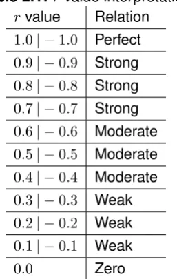
The interpretation ofKRCC andSRCC is discussed in [41]. In this paper both

coeffi-cients are referred to asrvalues. The interpretation of thisrvalue is different depending on

the research field. For example, anr value of0.7or−0.7(positive or negative correlation) is

defined asstrong,very strongand moderate for the respective fields of Psychology, Politics

[image:24.595.222.351.271.474.2]

and Medical. Since this project is focused on aggression, the ranges defined for Psychology are used in this project, see table2.1.

Table 2.1: rvalue interpretation rvalue Relation

0.0 Zero

Transitivity

Clinit Davis-Stober describes the transitivity of preference as follows: ”To have transitive preferences, a person, group, or society that prefers choice option x toy and y to z must

prefer x to z [42]. Furthermore a binary preference is defined as a preference choice

be-tween two alternatives, where one is chosen over the other. This can be transformed in the following statement:

∀x, y, zifxyandyzthenxz

If this proposition holds, this is perfect transitivity. Let matrix A be a preference matrix of

elementsa, b, c, d, e, whereais the most preferred option andethe least preferred option. If

matrixAis perfectly transitive, it would look like this:

A=        

0 1 1 1 1

0 0 1 1 1

0 0 0 1 1

0 0 0 0 1

0 0 0 0 0

(25)

2.8. BACKGROUNDRANKINGSTATISTICS 17

Whereaij = 1means thatij.When working with real world data, more often than not,

perfect transitivity cannot be assumed. To measure the level of in-transitivity, the preference

n∗nmatrix (P) can be compared to a referencen∗nmatrix (R) using the following formula:

Transitivity Error=

P

|P−R|

n2₋_n

In this formula the difference between the preference matrixP and the reference matrix R is divided by the amount of comparisons, excluding the diagonal because no element is

compared with itself.

To calculate the weight associated with elementxin matrixP, the sum of rowiis divided

by the sum of the full matrixP.

Wx=

P

jPx,j

P

i

P

jPi,j

The sample with the highest weight, will be the highest rank. If the situation of matrix A

would be a real world situation with a probability of0.1of an in-transitive preference, matrix

B could be the preference matrix of this situation.3

B =        

0 0.9 0.96 0.91 0.93 0.1 0 0.91 0.84 0.87 0.04 0.09 0 0.89 0.88 0.09 0.16 0.11 0 0.9 0.07 0.13 0.12 0.1 0

       

Transitivity Error=

P

|B−A|

52₋₅ = 0.101 The Transitivity Error is0.101≈0.1.

Wx=1= P

jP1,j

P

i

P

jPi,j

= 0.9 + 0.96 + 0.91 + 0.93

10 = 0.37

The weight associated with elementx= 1is0.37.

Multiple publications suggest that there can be in-transitivity when working with real world data [43]–[45], but no clear acceptable transitivity error is defined.

2.8.2 Rank Evaluation

(Mean) Average PrecisionIn information retrieval Mean Average Precision is widely used as an evaluation measure. Average Precision (AP) is ”the precision at each relevant [sam-ple], averaged over all relevant [samples]” [46]. This measure is mostly used in cases where

(26)

a binary relevant score is used(a document is either relevant or not). Mean Average Preci-sion(MAP) is AP averaged over multiple search queries. This is standard practice in Infor-mation Retrieval to validate a system. Since this project focuses on one query(aggression), MAP is less relevant.

Normalized Discounted Cumulative Gain (NDCG)When working with continuous rel-evance scores instead of binary relrel-evance scores, NDCG is a widely used measure in Infor-mation Retrieval [47]. Cumulative Gain is the sumInfor-mation over these scores up til a certain index. Discounted Cumulative Gain adds a penalty D for every index further up the list.

These measures are mostly used up until a certain point, indicated after the ’@’ sign.

Dr =

1 log(1 +r)

DCG@p=

p

X

r=1

IrDr= p

X

r=1

Ir

log(1 +r)

WhereIr is the relevance score of the sample at positionr in the ranking.

This measure can be normalized by dividing by DCG of the ideal ranking (IDCG), this measure is called Normalized Discounted Cumulative Gain (NDCG).

N DCG= DCG

(27)

Chapter 3

State of the Art

3.1 Aggression detection in audio

Kooij et al. [48] describe the development of CASSANDRA, a multi model system for surveil-lance purposes. The system uses 3D cameras in combination with audio classifiers in or-der to detect aggression. The audio component classifies audio as Speech, screaming, singing and ’kicking objects’. Furthermore, different audio features are extracted. The clas-sification labels, audio features and video features are combined using a Dynamic Bayesian Network(DBN) in order to determine the level of aggression. The Root Mean Squared Er-ror(RMSE) of the DBN while only using audio features is 0.223, where the full system, using all audio and visual features, yields an RMSE of 0.188.

3.2 State of the Art in Audio Annotation

In emotion annotation, including but not limited to the annotation of audio, the arousal-valance scale [6] is widely used [49], [50]. This scale used to be the state of the art anno-tation method, but a paradigm shift is taking place. Recent studies [51]–[58] show improved transitivity as well as improved accuracy when using ranked data sets, especially in affective computing.

Yang et al. [52], [53] describe two frameworks in which music is annotated in a ranking for both valence and arousal. In this framework annotators evaluate 8 randomly selected pairs of samples. The samples are compared as in a tournament, which leads to one final top sample. This way of annotating lowers the cognitive load, which makes it easier for annotators. Subjective evaluation of this annotation method, compared to a rating based annotation, showed positive results. On the other hand this only leads to most sample

and not to aleast sample, since in the tournament set up only the ’winning’ samples are

compared to each other in the next round. If this set-up would be extended so that the ’losing’ samples are compared to each other as well, the evaluation would also yield aleast

sample.

Yannakakis and Martinez [51] evaluate quality of different annotation methods on inter

(28)

20 CHAPTER3. STATE OF THEART

annotator agreement. They compared rating annotation with ranking annotation(both on arousal-valance scale) and found that ranking annotation improved inter annotator agree-ment. They extend their work in [57]. They state different disadvantages of rating based evaluation.

• Inter-personal difference; Two subjects may experience something(i.e. likability of a

sound) the same, but rate it differently. One subject might rate the sound as very likable where the other subject rates the sound as extremely likable.

• Ratings are transformed to numerical scales and used as interval, even though the

numerical scale is unknown. When subjects rate data through actual labels(i.e. Likert scale), the numerical scale of these labels is unknown, but the annotation is trans-formed assuming this numerical scale is known. Even when rating is done numerically, these values represent labels. For example ranging from very pleasant to not pleasant at all. Furthermore the assumption is made that this scale is linear, assuming that the distance between fairly pleasant (4) and moderately pleasant (3) is the same as the distance between fairly pleasant (4) and extremely pleasant (5).

On the other hand there is rank-based evaluation, which minimizes the assumptions that a subject has to make and is therefore a fairer evaluation. This is supported by Yannakis and Hallam [56], who compare rating-based and ranking-based evaluation. Within-subject analysis yielded higher in-transitivity for rating-based evaluation.

In an other study Martinez and Yannakakis [54] transform a rating based annotations into classes as well as into a ranking. They train a neural network to classify a sample as either more or less pleasant; by doing so, the model builds a ranking. Next to that they train a neural network to learn a ranking. Both systems are evaluated using Kendall’s Tau [59]. The ranking-based network outperformed the classification network.

3.2.1 Hybrid Comparison

(29)

3.3. STATE OF THEART INAUTOMATICAUDIORANKING 21

3.3 State of the Art in Automatic Audio Ranking

In audio ranking similar methods as for audio detection are applied. The research of Lot-fian and Busso [50] focuses on the comparison of ranking to two different types of Support Vector Machines (SVMs) in a speech recognition task. They investigate if Rank-SVMs can outperform ordinary SVMs and SVMs meant for regression (SVR).

To do so, the SEMAINE1_{database is used, which includes audio data that is annotated}

with absolute values for arousal and valance. A preference for each pair is determined by comparing these absolute values.

Evaluation is done according to median split. In fact it is a binary classification problem for a specific axis (arousal or valance), this makes it possible to use recall and precision as metrics.

All models use 50 high level descriptors as input. The rank-SVM outperforms both other models in this classification task. For arousal up to 20%, for valence with 7% and 4% for SVM and SVR respectively.

Parthasarathy, Lotfain and Busso [60] elaborate on their own work [50] by extending the work with DNNs. Ranknet is used to create a ranking of arousal, valence and dominance for a spoken conversation corpus. Ranknet outperforms RankSVM as well as the DNN regression model.

Yang et al. [61] use CNNs to predict hit rankings for Western and Chinese pop music. The target value of these songs is based on user listening data and used in a regression task. The hit score is calculated by multiplying a songs play count by the number of distinct users. In both of the subsets there are 10 thousand songs, 8 thousand are used for training, 1 thousand as validation and another 1 thousand as test set.

The study compares shallow networks and deep networks as well as two different types of inputs and the combination of these inputs. One of these inputs is the low-level mel-spectrogram. The other input is generated by using an auto-tagger that extracts 50 high level audio features of a sample. These features are used as input for the different neural networks.

Four metrics are used to evaluate the systems: Recall@1002_{; nDCG@100(which is}

similar to recall@100 but also takes the order of the recalled samples into account); Kendall’s Tau and Spearman’s Footnote.

The results show that deep models perform better than shallow models on the first two metrics. However on the two metrics that take the full ranking into account they score worse. The same goes for the auto-tagged input, this does have a positive effect on the metrics based on recall, but not on Kendall’s Tau and Spearman’s Footrule.

In two other studies [52], [53] applied learning-to-rank on similar data sets, only these data sets were human annotated. In this project the songs were annotated on the

(30)

22 CHAPTER3. STATE OF THEART

arousal scale, either as an absolute rating or through paired ranking. Two types of machine learning models were tested on this data set: a regression model and a list-wise learning-to-rank model. The paired-wise learning-learning-to-rank model is omitted in [53] because it is to computationally expensive(O(n(n−1))). In [52] pair-wise learning-to-rank is evaluated but

turns out to be highly time consuming.

In both experiments learning-to-rank outperforms the regression model, the best models achieving an accuracy of 73.6% for valance and 87.6% for arousal.3

Li [62] describes the use of point-wise, pair-wise and list-wise learning-to-rank for differ-ent applications. He states that there is no model that always outperforms the other two, but list-wise and pairwise usually outperform point-wise models. Furthermore the list-wise model approaches the learning problem more natural since it takes the ordered ground truth itself as a target variable. The results of Li are supported by Ghanbari [63], who investigates the effect of different loss functions.

3.4 Conclusion of State of the Art

Although rating-based annotation methods are still widely used, different studies show the improvements that can be made using ranking-based annotation methods. This same struc-ture is used in automatic ranking, including but not limited to audio. Learning-to-rank is widely used in information retrieval but has also gained attention in affective computing.

In this research the following ranking-based annotation methods will be investigated:

• Paired comparison. Two types of paired comparison will be investigated to find the

most efficient method, while still maintaining transitivity in the rankings. In the first method all samples will be pairwise compared. In the second method the binary search algorithm will be used to build a ranking, so that not all samples will be compared with each other explicitly.

• list-wise comparison. In this method the participant will evaluate more than 2 samples

will be ordered in a ranking. The combination of different lists will yield a final ranking. The results of the list-wise approach will be compared to the two paired comparison methods on time efficiency and transitivity.

The results will yield a balance between time efficiency and transitivity, based on which the best method is chosen and applied to a larger data set.

The larger data set will be used to evaluate a regression based machine learning model as well as a list-wise machine learning model, to investigate if audio samples can be ranked automatically based on aggression.

(31)

Chapter 4

Research Questions

4.1 Research Goals

Through this research we investigate a way to automatically rank audio files based on ag-gression. To do so a target ranking is needed, which can be used to train a machine learning model that can automatically rank audio files.

In this research two problems are discussed. The first problem is an annotation problem, where audio files have to be ordered based on aggression. In this project a system is developed that can be used to efficiently rank 3000 audio files based on aggression.

RQ1: How can a data set of 3000 audio files be annotated in a ranking in an efficient manner?

To answer this question, some sub questions must be answered.

SQ1.1: What is the level of transitivity in aggression annotation in audio samples? This question must be answered in order to determine if there is a logical order in audio files based on aggression. If humans cannot find an order, then it will not be possible to rank audio files on human annotations.

SQ1.2: How can audio samples be annotated into a ranking based on aggression?

SQ1.3: How efficient are the different types of audio annotation when ranking based on aggression?

By answering these questions on a small subset of the data, an efficient way of annotat-ing the entire data set can be found. When an efficient method is determined the data set will be annotated and can be used for automatic processing.

Another problem in this project is the automatic ranking of audio files. After the data is annotated, different machine learning techniques are evaluated for automatically rank audio files.

RQ2: How can audio samples automatically be ranked based on aggression? To answer this question, different sub questions are answered:

SQ2.1: How can regression be applied to rank audio files based on aggression?

(32)

24 CHAPTER4. RESEARCHQUESTIONS

SQ2.2: How can list-wise learning-to-rank be applied to rank audio files based on ag-gression?

(33)

Chapter 5

Research Methodology

5.1 How can 3000 audio files be annotated in a ranking in an

efficient manner?

The data set supplied by Sound Intelligence consists of roughly 3000 audio samples. To pairwise compare all files is not feasible, therefore two frameworks for building the ranked data set are proposed and tested.

5.1.1 Baseline

The baseline ranking is build using pairwise comparison, which is the most discriminat-ing way of compardiscriminat-ing audio samples into a rankdiscriminat-ing. For more information see chapter 2.1.2. This ranking is build using a pairwise comparison, in which the subjects have to compare the full matrix. In the first experiment 12 samples are evaluated, which lead to 66 comparisons(N(N −1)/2) for the baseline.

5.1.2 Binary Search

The first tested method is based on paired comparison and binary search explained in 2.1.3. The comparison is based on aggression. if the subject evaluates samplex more aggressive

than sampley, the algorithm will move up in the list. If the comparison is evaluated the other

way around, the algorithm will move down in the list.

5.1.3 Hybrid Comparison Insertion

This method is based on the hybrid comparison method explained in 3.2.1. It is not possible to let subjects make an ordered list of all the audio samples. In previous research partici-pants had to compare at most 12 samples at a time. To use this technique on a bigger data set, the existing ordered list is split into 12 parts. Of each part one sample will be used in a selection that has to be ranked by the participants. To this selection an unranked samplex

(34)

26 CHAPTER5. RESEARCHMETHODOLOGY

is added. The samples in between which xis ranked determine the new ordered list which

will again be split into 12 parts. This process will be repeated untilxhas a final position.

In order to simulate this ranking method while answering RQ1, the participant has to rank two lists of 7 samples in the first experiment. In these samples there will be two anchor samples, which occur in both lists. The anchors are obtained from the baseline. The lowest ranked sample and the highest ranked sample from the baseline will be used as anchors for the multi-list method.

Audio Samples12 audio samples are selected randomly from the labels human speech, raised voice and aggression. Of all three labels, four samples will be selected.

ParticipantsThe participants are naive subjects, in other words: not trained in audio annotation. The participants are students present at the University of Twente at the moment of the experiment. For each type of comparison, 25 subjects will take part in the experiment.

AnalysisThe results of the first experiment are validated based on transitivity and time efficiency.

Transitivity

Within every method, the following measures are compared. These measures should indi-cate if different participants agree with each other when using the same annotation tech-nique.

• transitivity(as explained in 2.8.1) within group

• Mean KRCC/SRCC within group (one vs rest)

The above two measures are useful to see the level of agreement within one method. If this differs over the ranking methods, this can be an argument to choose one over the oth-ers. Furthermore the methods are compared to the baseline results, which counts as a groundtruth for this experiment.

• transitivity compared to baseline.

• KRCC/SRCC compared to baseline

Literature suggests that a full paired comparison yields the most transitive and discriminating results. This analysis should find a more efficient method that achieves similar results as the baseline.

Time spend

time cost is rated using the following measures:

• Mean time spend(for 12 samples)

• Mean time spend per comparison

(35)

5.2. AUTOMATICRANKING OFAGGRESSION 27

• Time needed to annotate full and partial data set.

Based on the above measurements a simulation of the annotation process is done. The most important measurement is based on the quality of the ranking. To evaluate the quality, transitivity, KRCC andSRCC is used. Based on the values of these measures, the most

discriminating method is selected.

If these values are similar for multiple methods, time efficiency is used to select the best method. First, it the amount of comparisons needed to annotate 3000 samples is calculated for each individual method. The amount of comparisons multiplied by the time spend per comparison is used to give an indication of the time needed to annotate the full data set. Based on the combination of the quality of the ranking and the time needed to annotate a full ranking the most appropriate method is selected.

Ranking Simulation

When the most efficient ranking method is found, a simulation of the ranking process is done. this is used to find an indication of the expected in-transitivity for specific batch sizes, count of annotators and rank aggregation methods.

The simulation is done using a range of integers according to the different batch sizes. This range of integers is ranked using the most efficient ranking method. The simulation is done for different error rates, which defines the probability of a mistake: 0.05,0.1,0.15.

A mistake is defined as two samples that are not ordered in descending, but in ascending order.

The simulation is done using the following parameters:

• Batch size:10,50,100,200,300

• # annotators:3,5,10

• Rank aggregation methods: Mean, Mode, Median

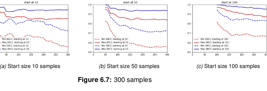
Furthermore, a simulation of the extension of the first batch ranking is done. In this simulation a start batch of size 10,50 or100is generated using the best rank aggregation

method and optimal annotator count. This ranking is used to add new files 1 by 1, based on the agreement of multiple annotators.

5.2 Automatic Ranking of Aggression

5.2.1 Data

(36)

The recordings in database A are recorded in healthcare institutions, the recordings in database B are recorded in prisons, the recordings in database C are recorded in an exper-tise centre for epilepsy. The recordings within a database can be very similar. Furthermore it is difficult to compare recordings from outside of a specific database, if most of the other samples are from the same database. Therefore a maximum number of recordings from these three main databases is set. The diversity in sources yields a diversity in audio frag-ments, which improves the generalizability of machine learning models.

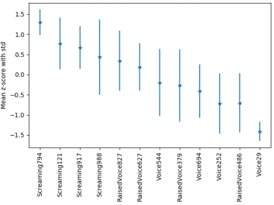
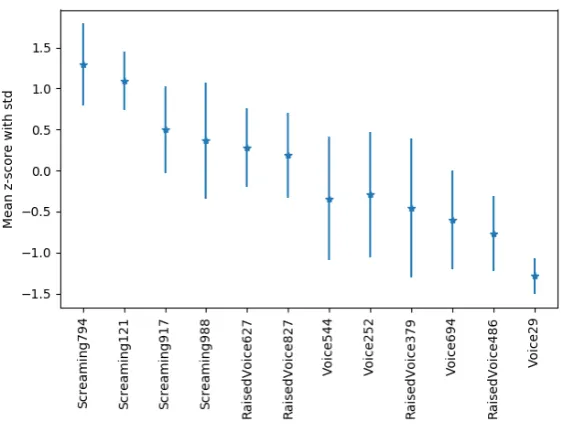
The full data set consist of 2427 audio samples drawn from the Sound Intelligence databases. The data is labelled by a group of trained annotators. The annotators select the part of an audio sample in which an event occurs and giving this part the appropriate label. The selected part of the audio is saved with the label. The labels used in this re-search areVoice,Raised VoiceandScreaming. The samples are drawn using the following

conditions:

• A maximum of 1000 files is randomly drawn from each of the following categories:

Voice,Raised VoiceandScreaming, since these categories are relevant for aggression

detection. Furthermore, these categories are used in the current aggression detection model.

• A maximum of 1₃ samples in each category may come from database A.

• A maximum of 1₃ samples in each category may come from database B.

• A maximum of 1₃ samples in each category may come from database C.

• The other samples come from diverse sources.

A final ranking is obtained by applying the annotation method developed answering Re-search Question 1, 5.1.

5.2.2 Data Analysis

The rankings of different annotators are compared to determine if a final ranking can be obtained that can be used to train and validate machine learning models. This final ranking should be acceptably transitive. It can be assumed that there is some degree of in-transitivity when working with real world data. Furthermore, the individual rankings should be positively correlated with each other. This indicates that the different annotators agree on the order of the recordings based on aggression. Therefore the rankings are individually compared with each other on KRCC, SRCC and in-transitivity. These measures are explained in 2.8.1.

Furthermore, the annotations are used to build four matrices and used to compare the individual annotations.

• Weighted Matrix, this is the matrix obtained by transforming every individual ranking

(37)

5.2. AUTOMATICRANKING OFAGGRESSION 29

• Linear Matrix, this is the reference matrix obtained by the ranking of the Weighted

matrix. Note that this matrix is perfectly transitive.

• Median Matrix, this is the paired matrix that follows from the final ranking, obtained by

aggregating the individual rankings using the median position of every sample.

• Median Matrix(equal allowed), this is the paired matrix similar to the median matrix

only now shared positions are allowed. If two samples share a position, the position in the matrix takes a value of0.5.

More information on these matrices can be found in 2.8.1.

Next to the individual rankings, the individual sample will be analyzed. It is assumed that the samples that are difficult to rank, will be ranked far apart over the different rankings. Based on the standard deviation of individual samples in the different rankings, a list of difficult to rank samples is specified.

The median ranking are used as a target for the machine learning models. For the regression model, the position of a sample is divided by the length of the ranking. This yields a value between 0 and 1 which can be used as a target value. For the list-wise learning-to-rank approach, a scoring function per sample is optimized, which gives a high value to relevant samples and a low value to irrelevant samples, so that the samples are ordered from most aggressive to least aggressive.

5.2.3 Audio Ranking using Machine Learning

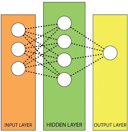
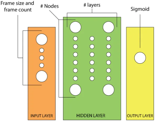
When applying fully connected Neural Network architectures it is important to supply the architecture with an input of the same size for every data point. Figure 5.1 shows the archi-tecture of a fully connected neural network with an input layer, 1 hidden layer and an output layer. The size of the input in this example is 3 nodes. This means that every data point that goes through this network, should be represented as a vector of length 3.

The data set used in this project consists of audio recordings of different lengths. All recordings are sampled at the same frame rate. Therefore the data points of this this data set all have different lengths, and should be processed before they can be supplied to an NN architecture. The problems that occur in the processing of unequal length audio samples are explained in 2.4.4.

Furthermore, the recordings will be annotated at clip level, which means it is unclear in which part of the recording the actual aggression occurs. This might not be a problem because the recordings are already trimmed to the event of the original label(Voice,Raised VoiceorScreaming), but the new annotation would still be classified as clip level annotation.

More information on weakly labeled data can be found in 2.4.3.

(38)

[image:38.595.173.395.83.312.2]

Figure 5.1:Fully Connected NN with an input layer of length 3.

value. The predicted value of the different frames of a specific recording are averaged to predict the value of a full recording. It is assumed that most information about aggression will be in the frames with the most energy. Therefore the predicted value is weighted by the energy of that sample to determine the average predicted value for each recording. This is done to deal with the weak labels. These values are compared to the unweighted predicted values for each recording to see if this leads to improvements in performance.

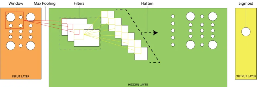
The wave recordings are sampled at a frame rate of 8000Hz and transformed into Log-Mel-Spectrums(LMS) of different frame sizes. These frame sizes are optimized during hyper parameter optimization. Next to the LMS of the current frame, the feature vector includes the LMS of previous frames, this is added to the current frame. The amount of frames in one feature vector is optimized during hyper parameter optimization.

The error function of the regression model is based on the distribution of the target values. As explained in 2.6.1, Mean Squared Loss is useful if the distribution of target values approaches the normal distribution, while Mean Squared Logarithmic Loss is more resistant to outliers.

The error function of the list-wise model is the Likelihood Loss explained in 2.6.2.

5.2.4 Performance