Data Mining Using Intelligent Systems: an
Optimized Weighted Fuzzy Decision Tree
Approach
By
XuQin Li
A thesis submitted in partial fulfillment of the requirements for the degree of
Doctor of Philosophy
School of Engineering
List of Figures ... 6
List of Tables ... 9
Acknowledgements ... 10
Declaration ... 11
List of Publications ... 12
Abstract ... 14
Abbreviations ... 16
Chapter ONE Introduction to Mata Mining
... 181.1 Introduction to data mining ... 18
1.2 Data Mining and Knowledge Discovery in Databases ... 19
1.3 Data mining challenges ... 22
1.3.1 High Dimensionality ... 22
1.3.2 Heterogeneous and complex data ... 22
1.3.3 Non-traditional analysis ... 23
1.4 Data mining tasks ... 23
1.5 Intelligent data mining techniques ... 26
1.6 Research objectives ... 28
1.7 Thesis outline ... 29
Chapter TWO Introduction to Intelligent Systems Techniques
... 322.1 Artificial neural network introduction ... 32
2.1.1 Multilayer Perceptron (MLP) ... 35
2.2.2 Self-organizing map (SOM) ... 38
2.2 Fuzzy logic ... 41
2.2.1 Fuzzy sets ... 41
2.2.5 Fuzzy C-means algorithm ... 47
2.3 Decision Tree ... 50
2.3.1 Introduction to the decision tree ... 50
2.3.2 How to build a tree ... 52
2.3.3 Design issues of decision tree induction ... 53
2.3.4 Measures for selecting the best split ... 53
2.3.5 Pruning the tree ... 55
2.3.6 Classify a new instance ... 57
2.4 Other Hybrid intelligent systems techniques ... 57
2.4.1 ANFIS ... 58
2.4.2 Evolving Fuzzy Neural Network (EFuNN) ... 60
2.4.3 Fuzzy ARTMAP ... 63
2.4.4 GNMM ... 65
2.5 Challenges of Knowledge Presentation ... 66
2.6 Datasets ... 67
2.7 Summary ... 70
Chapter THREE Improving Classification Rate Using Optimized
Weighted Fuzzy Decision Tree
... 783.1 Introduction ... 78
3.2 Fuzzy Decision Tree Algorithm ... 79
3.2.1 ID3 Algorithm Introduction ... 79
3.2.2 Construction of a Fuzzy Decision Tree Based on Fuzzy ID3 ... 81
3.2.3 Fuzzy Decision Tree Inference Mechanism ... 84
3.3 Optimized Weighted Fuzzy Decision Tree ... 86
3.3.1 Fuzzify Input ... 88
3.3.2 Modified Weighted Fuzzy Production Rules ... 89
3.3.3 Mapping weighted fuzzy Decision Tree to Neural Networks ... 90
3.5 Conclusion ... 99
Chapter FOUR Pattern Recognition of Fiber-Reinforced Plastic
Failure Mechanism: Using Intelligent Systems Techniques
... 1044.1 Introduction ... 104
4.2 Test Apparatus and Procedure ... 105
4.2.1 Acoustic emission equipment ... 105
4.2.2 Test procedure ... 107
4.3 Data Analysis ... 108
4.4 Test Results ... 113
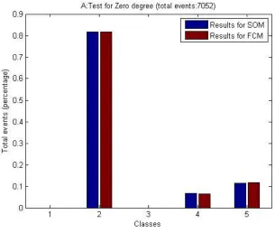
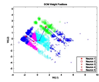
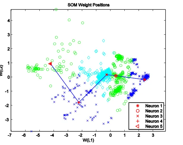
4.4.1 0° Fiber orientation ... 115
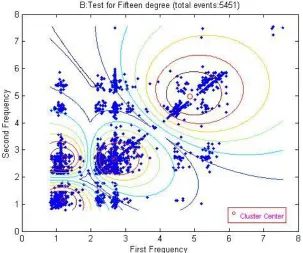
4.4.2 15° Fiber orientation ... 121
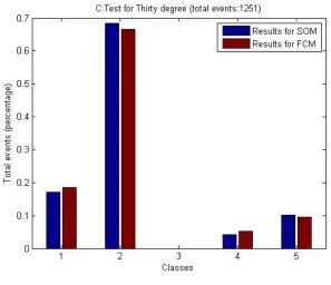
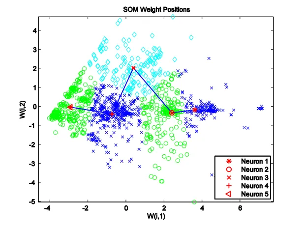
4.4.3 30° Fiber orientation ... 124
4.4.4 45° Fiber orientation ... 126
4.4.5 60° Fiber orientation ... 129
4.4.6 75° Fiber orientation ... 131
4.4.7 90° Fiber orientation ... 133
4.5 Discussion and Conclusions ... 136
4.6 Classifier design using Optimized Weighted Fuzzy Decision Tree ... 143
4.6.1 Fuzzy decision tree growing ... 144
4.6.2 Optimized weighted fuzzy decision tree ... 145
4.6.2.1 Fuzzify input ... 145
4.6.2.2 Mapping weighted fuzzy decision tree to neural networks and the learning process ... 146
4.6.3 Reasoning mechanism ... 147
4.6.4 Simulation Results ... 148
Bagging to Multilayer Perceptron and Decision Tree
... 1545.1 Introduction ... 154
5.2 Experiment and Data Collection ... 155
5.2.1 Instrumentation ... 155
5.2.2 Experimental Materials ... 156
5.3 Data Collection and Processing ... 157
5.4 Introduction to the classification techniques ... 160
5.4.1 General bootstrap methodology and bootstrap aggregation ... 161
5.5 Simulation Result ... 162
5.5.1 Using MLP as base classifier ... 162
5.5.2 Using Decision tree as the base classifier ... 167
5.6 Feature selection ... 172
5.7 Classifier design using Optimized Weighted Fuzzy Decision Tree ... 176
5.7.1 Fuzzify input ... 176
5.7.2 Reasoning mechanism ... 177
5.7.2 Simulation Results ... 178
5.8 Conclusion ... 179
Chapter SIX Classification of CLASH Dataset Using OWFDT and other
Intelligent Systems Techniques
... 1846.1 Introduction and motivation ... 184
6.2 Dataset ... 184
6.2.1 Output parameter ... 186
6.2.2 Preprocessing the data according to the Froude model scaling ... 187
6.3 Neural Network Simulation results ... 191
6.4 OWFDT results ... 196
6.5 Simulation results of other benchmarking techniques ... 198
6.5.1 ANFIS ... 198
6.5.2 EFUNN ... 204
6.6 Conclusion ... 211
Chapter SEVEN Conclusions and Suggestions for Future Work
... 2187.1 Overview of main research results ... 218
7.1.1 Optimized Weighted Fuzzy Decision Tree ... 218
7.1.2 Case study results ... 219
7.1.2.1 Composite material failure mechanism classification ... 219
7.1.2.2 Eye bacteria dataset ... 220
7.1.2.3 OWFDT case study results ... 220
7.2 Advantages and Disadvantages ... 221
Figure 1-1: KDD and intelligent systems techniques ... 20
Figure 1-2: Four of the core data mining tasks (excerpt from Tan, et al., 2005) ... 24
Figure 2-1: Basic architecture of a typical neural network ... 33
Figure 2-2: An example artificial neuron ... 34
Figure 2-3: Schematic of a Self Organizing Map topology ... 39
Figure 2-4: the Architecture of a basic Decision Tree ... 51
Figure 2-5: A comparison of three different impurity measures ... 55
Figure 2-6: A six layer ANFIS structure ... 59
Figure 2-7: Architecture of Evolving Fuzzy Neural Network (N. Kasabov, 2007) ... 60
Figure 2-8: Fuzzy ARTMAP architecture (Mannan, Roy, & Ray, 1998) ... 64
Figure 3-1: the architecture of a Fuzzy Decision Tree ... 84
Figure 3-2: The Mapping Structure from FPR to Neural Network ... 91
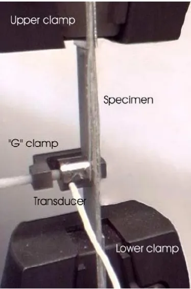
Figure 4-1: Test configuration, sensor coupled to the specimen using a G clamp... 108
Figure 4-2: (a), (top) waveform of a transient acoustic event; (b) (bottom) FFT power spectrum ... 109
Figure 4-3: Relationship between the 1st and 2nd highest power frequencies ... 111
Figure 4-4: PCA for the frequencies from Glass/Polyester 0° ... 112
Figure 4-5: Diagram of fiber orientations ... 113
Figure 4-6: Behaviour of fibre pull out for three different configurations, 0°, 30° and 90° Glass/Polyester subjected to tensile load ... 114
Figure 4-7: SOM output for 0° Glass/Polyester ... 116
Figure 4-8: SOM Neighbor Weight Distances ... 117
Figure 4-9: SOM sample hits for each neuron ... 118
Figure 4-10: Clustering indexes showing the No. of classes versus the index ... 119
Figure 4-11: FCM output for 0° Glass/Polyester ... 121
Figure 4-12: Normalized events per class for 0° Glass/Polyester ... 121
Figure 4-16: SOM output for 30° Glass/Polyester ... 125
Figure 4-17: FCM output for 30° Glass/Polyester ... 125
Figure 4-18: Normalized events per class for 30° Glass/Polyester ... 126
Figure 4-19: SOM output for 45° Glass/Polyester ... 127
Figure 4-20: FCM output for 45° Glass/Polyester ... 128
Figure 4-21: Normalized events per class for 45° Glass/Polyester ... 128
Figure 4-22: SOM output for 60° Glass/Polyester ... 129
Figure 4-23: FCM output for 60° Glass/Polyester ... 130
Figure 4-24: Normalized events per class for 60° Glass/Polyester ... 130
Figure 4-25: SOM output for 75° Glass/Polyester ... 132
Figure 4-26: FCM output for 75° Glass/Polyester ... 132
Figure 4-27: Normalized events per class for 75° Glass/polyester ... 133
Figure 4-28: SOM output for 90° Glass/Polyester ... 134
Figure 4-29: FCM output for 90° Glass/Polyester ... 135
Figure 4-30: Normalized events per class for 90° Glass/Polyester ... 135
Figure 4-31: Comparison of results for the 7 tests ... 137
Figure 4-32: SEM image of the 0° Glass/Polyester test (left: from the upper face of, right: from side of the failure zone)(Jimenez, 2007) ... 140
Figure 4-33: SEM image from the failure zone of Glass/Polyester test (left: 75°, right: 60°)(Jimenez, 2007) ... 140
Figure 4-34: SOM output for 0/90° Glass/Polyester ... 141
Figure 4-35: FCM output for 0/90° Glass/Polyester ... 142
Figure 4-36: Normalized events per class for 0/90° Glass/Polyester ... 142
Figure 4-37: Architecture of FDT for Zero Degree Dataset ... 144
Figure 4-38: Neural Network Structure of Mapped FPR ... 146
Figure 5-1: Statistical values for the dataset. ... 159
Figure 5-5: Classification tree structure before pruning ... 168
Figure 5-6: The estimated error for cross validation and resubstitution ... 170
Figure 5-7: The optimal tree with nine terminal nodes after pruning ... 171
Figure 5-8: Misclassification error cost curve ... 172
Figure 5-9: Feature importance histogram ... 174
Figure 5-10: Regression of test and validation data using selected features ... 175
Figure 6-1: Statistical characteristics for the dataset ... 190
Figure 6-2: Principal component analysis for the dataset ... 191
Figure 6-3: RMSE VS number of hidden neurons ... 194
Figure 6-4: Training performance of neural networks ... 195
Figure 6-5: Regression results for 1) training, 2) validation, 3) test and 4) all the datasets ... 196
Figure 6-6: Overview of ANFIS structure ... 199
Figure 6-7: ANFIS prediction results and error distribution ... 200
Figure 6-8: Rule extracted from ANIFS system ... 200
Figure 6-9: ANFIS rule viewer ... 202
Figure 6-10: Membership function for attribute 9 ... 202
Figure 6-11: ANFIS rule surface viewer ... 203
Figure 6-12: EFuNN prediction results and targets ... 205
Figure 6-13: Rules exacted from EFuNN system ... 205
Figure 6-14: Estimated error for cross validation and resubstitution ... 207
Figure 6-15: The pruned tree view ... 207
Table 3-1: Summary of the Datasets Employed ... 97
Table 3-2: Testing accuracy of the employed datasets (in percentage) ... 98
Table 3-3: Training epochs of WFDT and OWFDT ... 98
Table 4-1: Similarity Comparison of Two Results by FCM and SOM ... 138
Table 4-2: Testing Accuracy for the material datasets ... 149
Table 5-1: MME vs. Accuracy ... 166
Table 5-2: MME vs. Accuracy ... 175
Table 6-1: Parameters in the dataset and their function in the application ... 186
Table 6-2: parameter scaling according to Froude model law ... 188
Table 6-3: Statistical characteristics for the dataset ... 189
Table 6-4: Comparison of different IST results for CLASH data ... 211
I would like to express my sincere appreciation to my supervisor, Prof. Evor L. Hines for
his wonderful support, excellent supervision and endless guidance during the entire
period of my PhD studies and writing of this thesis. I would also like to extend my
sincere gratitude to Dr. Mark S Leeson for his kind assistance, advice and
encouragement for my research work.
I would also like to thank my wife, Min, for her support and tolerance of my PhD study,
as well as all night companionship during the past several years. Special thanks go to my
parents, parents-in-law and my sister for their help and support that they have given me
in so many ways through the good and bad times.
Thanks also go to Dr. Jianhua Yang, Dr. Harsimrat Singh, Mr. Huseyin Kusetogullari, Mr.
Reza Ghaffari and Dr. Wei Ren at the School of Engineering for their fruitful discussion
and support.
Last but not least, I thank the financial support from the Warwick Postgraduate
Research Fellowship (WPRF) and UK Overseas Research Students Awards Scheme
This thesis is presented in accordance with the regulations for the degree of doctor of
philosophy. The work described in this thesis is entirely original and my own, except
Book Chapters
XuQin Li, Evor L. Hines, Mark S. Leeson, Daciana. D. Iliescu, (2010), “Enhancing the classification of Eye Bacteria Using Bagging to Multilayer Perceptron”. Intelligent Systems for Machine Olfaction: Tools and Methodologies, Medical Information Science Reference.
Xu-Qin Li, M. S. Leeson, E. L. Hines, D. S. Huang, J. Yang, (2010), “Neural Networks for Solving Linear and Quadratic Programming Problems with Modified Newton's and Levenberg-Marquardt Methods”, in ‘Advances in Mathematics Research’, Volume 11, Editors: A. R. Baswell, Nova Publishers;
XuQin Li, Carlos Ramirez, Evor L. Hines, Mark S. Leeson, Phil Purnell, and M. Pharaoh, (2008), “Discriminating Fiber-Reinforced Plastic Signatures Related to Specific Failure Mechanisms: Using Self-Organizing Maps and Fuzzy C-Means”, intelligent systems: Techniques and Applications,Shaker Publications;
Jianhua Yang, Evor. L. Hines, Ian. Guymer, Daciana Iliescu, Mark. S. Leeson, G. P. King and XuQin. Li, (2007), “A Genetic Algorithm-Artificial Neural Network Method for the Prediction of Longitudinal Dispersion Coefficient in Rivers”, Advancing Artificial Intelligence through Biological Process Applications, Medical Information Science Reference;
Journal Papers
Intelligent and fuzzy system
Conference Papers
Data mining can be said to have the aim to analyze the observational datasets to find relationships and to present the data in ways that are both understandable and useful. In this thesis, some existing intelligent systems techniques such as Self-Organizing Map, Fuzzy C-means and decision tree are used to analyze several datasets. The techniques are used to provide flexible information processing capability for handling real-life situations. This thesis is concerned with the design, implementation, testing and application of these techniques to those datasets. The thesis also introduces a hybrid intelligent systems technique: Optimized Weighted Fuzzy Decision Tree (OWFDT) with the aim of improving Fuzzy Decision Trees (FDT) and solving practical problems.
This thesis first proposes an optimized weighted fuzzy decision tree, incorporating the introduction of Fuzzy C-Means to fuzzify the input instances but keeping the expected labels crisp. This leads to a different output layer activation function and weight connection in the neural network (NN) structure obtained by mapping the FDT to the NN. A momentum term was also introduced into the learning process to train the weight connections to avoid oscillation or divergence. A new reasoning mechanism has been also proposed to combine the constructed tree with those weights which had been optimized in the learning process. This thesis also makes a comparison between the OWFDT and two benchmark algorithms, Fuzzy ID3 and weighted FDT.
the patterns and predict the classes although OWFDT was used to design classifiers for all the datasets. In the material dataset, Self-Organizing Map and Fuzzy C-Means were used to cluster the acoustic event signals and classify those events to different failure mechanism, after the classification, OWFDT was introduced to design a classifier in an attempt to classify acoustic event signals. For the eye bacteria dataset, we use the bagging technique to improve the classification accuracy of Multilayer Perceptrons and Decision Trees. Bootstrap aggregating (bagging) to Decision Tree also helped to select those most important sensors (features) so that the dimension of the data could be reduced. Those features which were most important were used to grow the OWFDT and the curse of dimensionality problem could be solved using this approach. The last dataset, which is concerned with wave overtopping, was used to benchmark OWFDT with some other Intelligent Systems techniques, such as Adaptive Neuro-Fuzzy Inference System (ANFIS), Evolving Fuzzy Neural Network (EFuNN), Genetic Neural Mathematical Method (GNMM) and Fuzzy ARTMAP.
AE Acoustic Event AI Artificial Intelligence AN Artificial neuron
ANFIS Adaptive Neuro-Fuzzy Inference System ANN Artificial Neural Network
ART Adaptive Resonance Theory BCI Brain-Computer Interface BP Back-Propagation
CART Classification and Regression Tree CSP Common Spatial Patterns
DM Data Mining DT Decision Tree
ECoG Electrocorticography EEG Electroencephalogram
EFuNN Evolving Fuzzy Neural Network EN Electronic Nose
FCM Fuzzy C-Means FDT Fuzzy Decision Tree
FFT Fast Fourier Transformation FIS Fuzzy Inference System FL Fuzzy Logic
GNMM Genetic Neural Mathematical Method ICA Independent Component Analysis ID3 Iterative Dichotomizer 3
IS Intelligent System
IST Intelligent Systems Technique KDD Knowledge Discovery from Data LM Levenberg-Marquardt
MF Membership Function MLP Multi-Layer Perceptron MSE Mean Square Error NN Neural Network
OWFDT Optimized Weighted Fuzzy Decision Tree PCA Principal Components Analysis
PNN Probabilistic Neural Network PR Pattern Recognition
RBF Radial Basis Function
SEM Scanning Electron Microscope SC Soft Computing
SOM Self-Organizing Map
18
Chapter I: Introduction to Data Mining
1.1 INTRODUCTION TO DATA MINING
1.2 DATA MINING AND KNOWLEDGE DISCOVERY IN DATABASES
1.3 DATA MINING CHALLENGES
1.4 DATA MINING TASKS
1.5 INTELLIGENT DATA MINING TECHNIQUES
1.6 RESEARCH OBJECTIVES
1.7 THESIS OUTLINE
1.1 Introduction to data mining
Advances in data collection and storage technology have enabled researchers to
accumulate vast amounts of data. With the enormous amount of data stored in files,
databases, and other repositories, researchers from many areas have been stimulated
to adopt and develop new techniques for data analysis in different fields of science.
Powerful means of analyzing, interpreting and extracting interesting knowledge that
could help in decision-making processes have also been designed (Gaber, 2010). Data
mining is such a technology that combines data analysis methods (intelligent systems
19
Data mining is the process of applying neural networks, clustering, fuzzy logic and
decision tree etc. to data with the intention of uncovering hidden patterns and
extracting information (Kantardzic, 2002). It involves an integration of these different
techniques from different disciplines which can facilitate the extraction of knowledge
from a large amount of data (Tan, Steinbach, & Kumar, 2005).
1.2 Data Mining and Knowledge Discovery in Databases
The term ‘data mining’ is often regarded as an integral part of Knowledge Discovery in
Databases (KDD), which is overall process of extracting implicit, previously unknown and
potentially useful information from raw data (Larose, 2005). There have been notable
successes in the use of statistical, computational and machine learning techniques to
discover scientific knowledge in the field of engineering, biology, medicine and physics
etc.
The KDD process consists of applying data analysis and computing algorithms which
produce a particular enumeration of patterns over data. In addition to that, KDD will
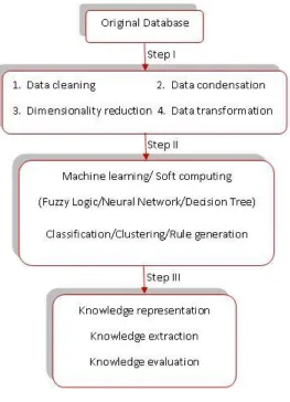
also discover regularities to improve future decisions. Figure 1-1 shows the relationship
between KDD and intelligent systems techniques (Venugopal, G.Srinivasa, & Patnaik,
20
Figure 1-1: KDD and intelligent systems techniques
The steps in the KDD process are briefly explained below (Venugopal, et al., 2009):
The first step is concerned with data preprocessing which consists of the following four
elements:
Data cleaning to remove noise and irrelevant data from collection;
Data integration which involves combining of multiple and heterogeneous data
sources;
Data selection where data relevant to analysis task is retrieved from the
21
Data transformation where consolidated data is transformed into forms
appropriate for the mining procedure;
The second step is concerned with data mining process which consists of the following
two elements:
Data mining which is essential and where intelligent systems techniques are
applied in order to discover and extract patterns from datasets;
Pattern evaluation where patterns representing knowledge are measured and
identified;
The third step is concerned with knowledge presentation which consists of the following
element:
Knowledge presentation where knowledge is presented to final users in a
visualized way to help them understand and interpret the mining results.
Although data mining is not isolated with data preprocessing and knowledge
presentation steps, this thesis will focus on the data mining process which involves
design and implementation of intelligent systems techniques.
Data mining is concerned with building models to determine patterns from observed
data. The models play the role of inferring knowledge. A model is simply an algorithm or
a set of rules that connects a collection of inputs to a particular target or output (Larose,
2006). Neural Networks, fuzzy inference systems, decision trees, regression and other
22
Linoff, 2004). Deciding whether the model reflects useful knowledge or not is a part of
the overall KDD process. But in order to evaluate the knowledge discovered in the KDD
process, the models are usually tested using a test dataset to evaluate the performance
of the models.
1.3 Data mining challenges
Although traditional data mining techniques have achieved great success, they also
encountered practical difficulties in meeting challenges posed by new type of datasets.
Pang-Ning Tan et al. had identified the following challenging problems: mainly high
dimensionality, heterogeneous and complex data and non-traditional analysis (Tan, et
al., 2005):
1.3.1 High Dimensionality
A data set may have hundreds or even thousands of attributes (features) compared to
several a few decades ago. One extreme exists in bio-informatics: microarray, consisting
of an array series of thousands of microscopic spots, each containing a specific DNA
sequence, has enabled gene expression in tens of thousands of features. For most of
data analysis algorithms, the computational complexity increases exponentially as the
dimensionality (the number of features) increases (Liu & Motoda, 2007).
1.3.2 Heterogeneous and complex data
Traditional datasets often contain attributes of the same type, either continuous
23
science, engineering, bio-informatics, medicine and other fields have grown, the need
for techniques that can deal with heterogeneous attributes has also risen. Recent years
have also seen the emergence of more complex data objects.
1.3.3 Non-traditional analysis
The traditional analysing approach is based on a hypothesize-and-test paradigm. In
other words, the experiment design and data analysis are both related to the hypothesis.
But this process can be extremely labour-intensive and could even stop working if the
number of hypothesis and test paradigm is in the thousands (Cao, Wegman, & Solka,
2005). As a result, there is no hypothesis-and-test procedure in the data mining and the
process of hypothesis generation and evaluation is automatically incorporated in the
algorithms.
1.4 Data mining tasks
Data mining tasks are generally divided into two major categories: predictive and
descriptive. The former aims to predict the value of a particular attribute (target or
dependent variable) based on values of other attributes and the latter will derive
patterns (correlations, trends, clusters, trajectories and anomalies) which can typically
denote the underlying relationships in data (Tan, et al., 2005).
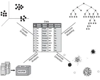
Figure 1-2 shows four of the core data mining tasks. Predictive modelling and cluster
24
Figure 1-2: Four of the core data mining tasks (excerpt from Tan, et al., 2005)
Association analysis aims at discovering patterns that lay behind the datasets and
describing associated features in the data. The patterns discovered can typically be
represented either in the form of implication rules or feature subsets (Lawrence, Kudyba,
& Klimberg, 2008). The goal of association analysis is to extract the most interesting and
representative patterns in an effective manner (Dunne, 2007).
Anomalies are also referred to as outliers. Anomaly detection, sometimes referred to
as outlier detection, involves detecting instances in a given dataset that do not conform
to a pre-defined class set or identifying cases that are unusual with the dataset that is
seemingly homogeneous. Anomaly detection is a very important tool in a variety of
25
Predictive modelling involves building a model to predict the target variable as a
function of the explanatory variables (Larose, 2006). Two typical types of predictive
modelling tasks are classification and regression. The former is used for discrete target
variables and the latter is used for continuous target variables.
Classification is one of the most common tasks in the data mining domain discussed in
this thesis. It consists of examining the attributes of a newly presented instance and
assigning it to one of a predefined set of classes. The classification task is characterized
by a well-and-pre-defined definition of the classes, and a training data set consisting of
pre-classified examples (Hand, Smyth, & Mannila, 2001). The task of classification is to
build a model that can be applied to unclassified data instance in order to classify this
unseen instance (Larose, 2006).
Cluster analysis seeks to segment heterogeneous observations into a number of more
homogeneous subgroups or clusters. Usually, the observations are grouped together
based on self similarities, so observations that belong to the same cluster are most
similar to each other than observations that belong to other clusters (Witten & Frank,
2005).
A class is a set of data samples with some similarity or relationship and all samples in
this class are assigned the same class label to distinguish them from samples in other
classes. A cluster is a collection of objects which are similar locally. Clusters are usually
generated in order to further classify objects into relatively larger and meaningful
26
the clustering process doesn’t assign and rely on a predefined class set. But in
classification, each new instance is classified into a predefined class through some
intelligent systems techniques which are trained with some predefined instances.
Clustering can be employed for dealing with data which have not been put into classes.
Some classification methods cluster data into small groups first before proceeding to
classification (Berry & Linoff, 2004). In the context of intelligent systems technique,
clustering can be regarded as a kind of unsupervised learning and classification can be
regarded as supervised learning.
This thesis will focus mainly on the following data mining tasks: classification and
clustering, prediction and rule extraction.
1.5 Intelligent data mining techniques
Data mining may be chosen to deal with datasets which contain a huge amount of data
and may be ambiguous and even partly conflicting. In order to make the data and
information mining process more robust, intelligent systems techniques for searching
and learning the data and information require tolerance toward imprecision,
uncertainty and exceptions. The intelligent systems incorporating these intelligent
systems techniques will have approximate reasoning capabilities and be capable of
handling partial truth (Han & Kamber, 2006). These are also some typical characteristics
27
Since there is no generic term for intelligent computing techniques used in data mining.
In this thesis, the term Intelligent Systems (ISs) will be used interchangeably with
intelligent systems techniques and soft computing, although under most circumstances,
Intelligent Systems (ISs) is preferred. Soft computing is an important technique domain
in the area of data mining and intelligent and knowledge-based systems (Karray & Silva,
2005). Soft computing differs from conventional (hard) computing because of its
tolerance of imprecision, uncertainty, partial truth and approximation. So the main
principle of soft computing is to exploit the tolerance for imprecision, uncertainty,
approximation and partial truth in order to achieve tractability, robustness and low-cost
solution (Han & Kamber, 2006; Venugopal, et al., 2009).
The principal computing paradigms of soft computing are fuzzy logic, neural networks,
probabilistic reasoning and genetic algorithms. These methodologies of soft computing
are complementary and cooperative rather than competitive and exclusive (Engelbrecht,
2002). A problem can be solved most effectively by combining different techniques such
as fuzzy logic, neural networks, genetic algorithms and probabilistic reasoning rather
than using them exclusively and individually. For example, ANFIS, which incorporates
fuzzy logic and neural networks, has proved to be successful for solving many practical
problems. These techniques can be viewed as a foundation component for intelligent
28
1.6 Research objectives
Each of the IS techniques contributes a distinct methodology for addressing problems in
its domain. This may be done in a cooperative, rather than a competitive, manner. The
result is a more intelligent and robust system providing a human-interpretable, low-cost,
approximate solution, as compared to traditional techniques (Ian & Jacek, 2000).
The unique contribution of this thesis is in the implementation of a hybrid IS DM
technique, which incorporates fuzzy logic, decision tree and neural networks, for solving
novel practical problems, the detailed description of this technique (Optimized
Weighted Fuzzy Decision Tree, OWFDT), and the illustrations of several applications
solved by Optimized Weighted Fuzzy Decision Tree.
The primary objective of this work is to design an IS system that can be applied
effectively to some DM tasks such as those listed in Figure 1-2. The devised intelligent
systems will also focus on solving the following issues particularly (Wang & Fu, 2005):
Achieve a high and acceptable classification or prediction accuracy;
Reduce the dimension of the data set and ease the computational complexity;
Extract some rules if applicable
The thesis also aims to explore the possibilities of applying this hybrid IS DM technique
to material, biological and civil engineering applications, since the problems in these
fields are quite complex and the datasets available are in massive quantities. This thesis
29
OWFDT. The thesis will also conduct a benchmark study between the proposed
technique and other techniques to test the performance of the newly-proposed
technique.
1.7 Thesis outline
Chapter one is a brief overview of data mining, including its concept, its challenges and
tasks. The research objective and overall structure of the thesis is also listed in this
chapter.
Chapter two gives a brief introduction to the theoretical background of the techniques
used in the thesis including fuzzy logic, neural networks (self-organizing map,
multiple-layer perceptron), decision tree and some other hybrid intelligent systems, such as
Adaptive Neuro-Fuzzy Inference Systems, Fuzzy ARTMAP etc.
Chapter three introduces the Optimized Weighted Fuzzy Decision Tree, which will be
used in the following chapters. A detailed description is presented first, and this is
followed by the simulation results after applying OWFDT to three datasets.
Chapter four analyzes the datasets collected from material science and clustered the
data in order to predict the possible composite material failure mechanism. The OWFDT
is also used to construct a classifier for prediction and classification of those failure
30
In chapter five an eye bacteria dataset collected using electronic nose is analyzed using
bagging to Multi-Layer Perceptron and Decision Tree. OWFDT is also adopted as an
intelligent systems technique to predict the eye bacteria species.
Chapter six is concerned with the analysis of a wave overtopping dataset and
conduction of a benchmark study between some well-established hybrid intelligent
techniques and OWFDT.
Chapter seven presents the conclusions and suggestions for further study.
References
Berry, M. J. A., & Linoff, G. S. (2004). Data mining techniques: for marketing, sales, and
customer relationship management: Wiley.
Cao, C. R., Wegman, E. J., & Solka, J. L. (2005). Handbook of Statistics: Data Mining and
Data Visualization: Elsevier North-Holland.
Dunne, R. A. (2007). A Statistical Approach to Neural Networks for Pattern Recognition:
John Wiley & Sons,.
Engelbrecht, A. P. (2002). Computational Intelligence: An Introduction. Chichester: John
Wiley.
Gaber, M. M. (2010). Scientific Data Mining and Knowledge Discovery: Principles and
Foundations: Springer-Verlag.
Han, J., & Kamber, M. (2006). Data mining: concepts and techniques. Amsterdam:
31
Hand, D. J., Smyth, P., & Mannila, H. (2001). Principles of data mining: MIT Press.
Ian, C., & Jacek, M. Z. (2000). Knowledge-based neurocomputing: MIT Press.
Kantardzic, M. (2002). Data Mining: Concepts, Models, Methods, and Algorithms:
Wiley-IEEE Press.
Karray, F. O., & Silva, C. W. D. (2005). Soft Computing and Intelligent Systems Design:
Theory, Tools and Applications: Addison-Wesley.
Larose, D. T. (2005). Discovering Knowledge in Data: An Introduction to Data Mining:
John Wiley & Sons, Inc.
Larose, D. T. (2006). Data Mining Methods and Models. New Jersey: John Wiley & Sons,
Inc.
Lawrence, K. D., Kudyba, S., & Klimberg, R. K. (2008). Data Mining Methods and
Application: Auerbach Publications Taylor & Francis Group.
Liu, H., & Motoda, H. (2007). Computational Methods of Feature Selection (Chapman \&
Hall/Crc Data Mining and Knowledge Discovery Series): Chapman \& Hall/CRC.
Tan, P.-N., Steinbach, M., & Kumar, V. (2005). Introduction to Data Mining, (First Edition):
Addison-Wesley Longman Publishing Co., Inc.
Venugopal, K. R., G.Srinivasa, K., & Patnaik, L. M. (2009). Soft Computing for Data Mining
Applications. New York: Springer-Verlag.
Wang, L., & Fu, X. (2005). Data Mining with Computational Intelligence (Advanced
Information and Knowledge Processing): Springer.
Witten, I. H., & Frank, E. (2005). Data mining : practical machine learning tools and
32
Chapter II: Introduction to Intelligent
Systems Techniques
2.1 ARTIFICIAL NEURAL NETWORK INTRODUCTION
2.2 FUZZY LOGIC
2.3 DECISION TREE
2.4 OTHER HYBRID INTELLIGENT SYSTEMS TECHNIQUES
2.5 CHALLENGES OF KNOWLEDGE PRESENTATION
2.6 DATASETS
2.7 SUMMARY
Chapter one has introduced the concept of data mining and outlined the research
objectives of the thesis. The current chapter will provide a solid theoretical background
of some intelligent systems techniques which are widely used in the subject of data
mining. This chapter will concentrate on these techniques including artificial neural
networks (NN), fuzzy logic (FL) and decision tree (DT) which are core techniques that
OWFDT is based on. The last section of this chapter will introduce some hybrid
intelligent systems techniques.
33
Neural networks (NNs) first started to be developed in the 1940s, motivated by, for
example, an attempt to simulate the human brain on computers. It has been
successfully applied to prediction problems, pattern recognition, classification and
optimization problems (Hagan, Demuth, & Beale, 1996; Haykin, 1999).
Usually, ANNs consist of simple parallel interconnected and usually adaptive processing
elements or neurons whose connectivity mimics the neurobiological system (Chow,
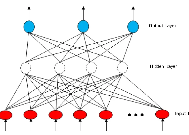
2007). These neurons are typically distributed over several layers. Forward Neural
Network (FNN) is one of the most popular network topologies. Normally, the neurons in
a FNN are arranged into three layers as shown in Figure 2-1. Neurons in each layer
perform a different activity as described in the following three steps (Kartalopoulos,
[image:34.612.131.459.404.639.2]1997):
34
(1) The input neurons receive information in the form of input values. They transfer the
data to the next layer. Neurons in the input layer perform no neural function.
(2) Hidden neurons receive the output from the input neurons or other hidden neurons
through the connections. Each connection between input neurons and hidden neurons
has a weight by which to multiply the signal before it enters the hidden neurons. A
hidden neuron usually receives more than one signal. The signals will be combined and
transferred to an appropriate activation function. The output of the activation function
will then be usually transferred to output neurons but sometimes via hidden neurons
(as shown in Figure 2-2). Figure 2-2 shows the structure and the function of a neuron.
Figure 2-2: An example artificial neuron
(3) Output layer neurons behave similarly to the ones in the hidden layer except that
the pattern of the outcome from output neurons may be interpreted as the outcome of
using the NN to process the input data.
Training the system is the key to determining whether or not the NN will be able to
process the input data appropriately. In a supervised NN the training process allows NNs
35
difference between the generated output and the desired output is called the “error”.
The NN will adjust the weight of each connection in such a way as to reduce the error
(Du & Swamy, 2006). At the beginning, the NN might produce a large error. However, if
the problem can be solved by NN then, after several cycles of training with the set of
data, the error should reduce.
Multilayer Perceptron (MLP) is one of fully connected FNN.
2.1.1 Multilayer Perceptron (MLP)
The multilayer perceptron (MLP) is able to learn arbitrarily complex non-linear
relationships. Usually a three-layer feed-forward network, MLP is the most popular type
of ANN in practical use. Figure 2-1 shows the structure of an MLP, in which the
processing elements are organized in a regular architecture (or topology) of three
distinct groups of neurons (input, hidden and output layer) interconnected using
unidirectional weights. The number of input nodes is typically set to correspond with
the number of dimensions in the problem. The number of neurons in the hidden layer is
determined experimentally and the number of output classes in the analyzed dataset
determines the number of outputs.
Each neuron in MLP performs a weighted sum of inputs and transforms it using a
nonlinear activation function (e.g. sigmoid transfer function) (Haykin, 1999). An MLP is
able to learn from data by adjusting the weights in the network using a gradient descent
technique known as back-propagation (BP) of errors. MLP adopts a supervised training
36
the network. During the forward pass, the MLP processes all of its input in a
feedforward manner; the output of each neuron is calculated and feeds the next layer
through to the output. Let us consider a neuron h, with jth input vector which consists
of n elements 𝑥𝑖𝑗(𝑖 = 1, … 𝑛), the summation function 𝑎𝑗 accumulates the sum of the
products of the input signals 𝑥𝑖𝑗 with associated weights 𝑤𝑖. It assumes a fixed
weight,𝜃, which is then transformed by the activation function f(.) (e.g. sigmoid) to
produce the single output 𝑧𝑗, the overall computations follows that given in equation
(1):
𝑧𝑗 = 𝑓 𝑎𝑗 = 1
1 + exp −𝑎𝑗 = 𝑓 𝑤𝑖𝑥𝑖𝑗 − 𝜃
𝑛
𝑖=1
(𝑖 = 1, … 𝑛)
(1)
The error is then calculated by determining the difference between the actual generated output 𝑧𝑗and the target output 𝑡𝑗using the expression 𝛿𝑗 = 𝑧𝑗 − 𝑡𝑗. The
error term is often called delta and hence when the delta learning rule is used, the
component difference expression becomes 𝛿𝑗 = (𝑧𝑗 − 𝑡𝑗)(1 − 𝑡𝑗). In the backward
pass, the stochastic approximation procedure back-propagates this error to adjust the weight values during each presentation of the jth training sample on each iteration (or epoch) 𝜏. Various training algorithms can be used to improve the operation of BP
37
BP gradient descent with momentum (BPGDM). The new set of weights
𝑤𝑗(𝜏) comprise of a combination of the old weight values, 𝑤𝑗(𝜏−1) (from the
previous epoch) and a weight update or delta, ∆𝑤𝑗(𝜏) (see equation (2)). The
change in weights here is based on two parameters; 1) 𝜂, the learning rate, a
small positive number (the default is generally 0.9) that determines the rate of
convergence to a solution of minimum error, and 2) 𝜇, the momentum term, a
small positive number (default is generally 0.5) is often added to improve the
speed and stability of the learning.
𝑤𝑗(𝜏) = 𝑤𝑗(𝜏−1)+ ∆𝑤𝑗(𝜏)= 𝑤𝑗(𝜏−1)− 𝜂𝛿𝑗𝑧𝑗(𝜏)+ 𝜇∆𝑤𝑗(𝜏−2) (2)
Faster BP training. BPGDM is often too slow for practical problems and other
high performance algorithms were introduced, such as conjugate gradient,
quasi-Newton and Levenberg-Marquardt (BPLM) (Chow, 2007; Ham & Kostanic,
2000). The BPLM was designed to approach a second-order training speed using
the Jacobian matrix J, which contains the first derivatives of the network errors
with respect to the weights and biases. The algorithm uses equation (3) where 𝜇
is an updating (decreasing) scalar.
𝑤𝑗(𝜏)= 𝑤𝑗(𝜏−1)− [𝐉T𝐉 + 𝛍𝐑
𝑗]−1𝐉T𝛿𝑗 (3)
Using BP, the weights and biases associated with the neurons are modified to minimize
the mapping error, when these stabilise, the network is said to be trained (the total sum
38
procedure is repeated for a number of epochs until the network error has fallen to a
small constant error level. Once the network is trained, it can be used to predict the
membership of unseen samples in a validation set. The classification of new patterns is
performed by propagating the new patterns through the network and the output
neuron with the highest score indicates the predicted class.
2.2.2 Self-organizing map (SOM)
Here Self-Organizing Map (SOM) was chosen as the structure of neural networks for
analyzing the material data set in the thesis, because it is an unsupervised learning
technique suitable for datasets with no pre-defined classes.
The SOM algorithm was developed by Kohonen to transform a data set of arbitrary
dimensions into a one or more dimensional discrete map(Kohonen T, 1990). According
to Kohonen, SOM’s are connectionist techniques capable of generating topology which
can preserve clustering information. An example of the network architecture of a
Kohonen SOM is shown in Figure 2-3 (Godin, Huguet, & Gaertner, 2005). It consists of a
two dimensional array of m x m discrete units and the Kohonen network associates each
39
Figure 2-3: Schematic of a Self Organizing Map topology
Suppose 𝑤𝑖𝑗are the components of the weight vector 𝑊𝑗, connecting the inputs i to
output node j; the 𝑥𝑖 are components of the input vector X, the output of the neuron is
the quadratic (Euclidean) distance 𝑑𝑗 between the weight vector and the input vector
(see Figure 2-3). The description of each step to use the data to train the SOM is
summarized as follows (Ham & Kostanic, 2000):
Initialize all the weights to random values between 0 and 1.
Randomly select an input vector X; present it to all the neurons of the network
and evaluate the corresponding quadratic distance output 𝑑𝑗 according to the
following equation:
40
where n is the number of input vector components.
Select the neuron with the minimum output 𝑑𝑗 as the wining neuron, i.e. the
nearest vector to the input vector. Let 𝑗∗denote the index of the winner, the
minimum output will be:
𝑑𝑗∗= min
𝑗 ∈[1,2,…,𝑚^2] 𝑋 − 𝑊𝑗 2
(5)
where m x m is the number of neurons.
Update the weight of the wining neuron according to Equation (6).
𝑤𝑖𝑗∗ 𝜏 + 1 = 𝑤𝑖𝑗∗ 𝜏 + 𝜂 𝜏 [𝑥𝑖 𝜏 − 𝑤𝑖𝑗∗ 𝜏 ] (6)
where 𝜏 is the learning iteration count and η is the gain term.
The neighbors of the wining neuron, defined by the neighborhood function 𝑁(𝑗∗) (the neighborhood function 𝑁(𝑗∗) defines how many neurons in the
neighborhood of the winning one will be updated for each learning input) are
also updated following Equation (7) and (8):
𝑤𝑖𝑗 𝜏 + 1 = 𝑤𝑖𝑗 𝜏 + 𝜂 𝜏 [𝑥𝑖 𝜏 − 𝑤𝑖𝑗 𝜏 ] (7)
If ∈ 𝑁(𝑗∗) , neighborhood of 𝑗∗
𝑤𝑖𝑗 𝜏 + 1 = 𝑤𝑖𝑗 𝜏 (8)
41
Repeat the learning process until all the input vectors X have been used at least
once.
2.2 Fuzzy logic
The concept of Fuzzy Logic (FL) was conceived by Lotfi Zadeh, a professor at the
University of California at Berkley, and presented as a way of processing data by
allowing partial set membership rather than crisp set membership or non-membership
(Babuska, 1998). It is basically a multi-valued logic that allows intermediate values to be
defined between conventional evaluations.
2.2.1 Fuzzy sets
A fuzzy set is a set without a crisp and clearly-defined boundary or without binary
membership characteristics. Unlike an ordinary set where each object (or element)
either belongs or does not belong to the set, fuzzy set can contain elements with only a
partial degree of membership. In other words, there is a ‘softness’ associated with the
membership of elements in a fuzzy set (Kartalopoulos, 1997). An example of a fuzzy set
could be ‘the set of tall people.’ There are people who clearly belong to the above set
and others that cannot be considered as tall. Since the concept of ‘tall’ is not precisely
defined (for example, >2m), there will be a gray zone in the associated set where the
membership is not quite obvious. As another example, consider the
variable ’temperature’. It can take a fuzzy value (e.g., cold, cool, tepid, warm, and hot).
42
fuzzy set because any temperature that is considered to represent ‘hot’ belongs to this
set and any other temperature does not belong to the set. A crisp set or a precise
temperature interval such as 25 °C to 30 °C cannot be indentified to represent warm
temperatures.
2.2.2 Membership function
A fuzzy set can be represented by a membership function. This function indicates the
grade (degree) of membership within the set, of any element of the universe of
discourse (e.g. the set of entities over which certain variables of interest in some formal
treatment may range). The membership function maps every element of the universe to
numerical values in the interval [0, 1]. Specifically,
𝜇𝐴 𝑥 : 𝑋 → 0, 1 (9)
where 𝜇𝐴 𝑥 is the membership function of the fuzzy set A in the universe X. Stated in
another way, fuzzy set A is defined as a set of ordered pairs (H. Li, Philip, & Huang, 2000):
𝐴 = { 𝑥, 𝜇𝐴 𝑥 ; 𝑥 ∈ 𝑋, 𝜇𝐴 𝑥 ∈ [0, 1]} (10)
The membership function 𝜇𝐴 𝑥 represents the grade of possibility that an element x
belongs to the set A. It is a curve that defines how each point in the input space is
mapped to a membership value. A membership function value of zero indicates that
corresponding element is definitely not an element of the fuzzy set. A membership
function value of unity implies that the corresponding element is definitely an element
43
non-crisp (or fuzzy) membership, and the corresponding elements fall on the fuzzy
boundary of the set. The closer the 𝜇𝐴 𝑥 is to 1 the more the x is considered to belong
to A, and similarly, the closer it is to 0 the less it is considered to belong to A.
The following is a summary of the characteristics of fuzzy set and membership function
(Tsoukalas & Uhrig, 1996):
Fuzzy sets describe vague concepts (e.g., fast runner, hot weather, and weekend
days).
A fuzzy set admits the possibility of partial membership in it. (e.g., Friday is sort
of a weekend day, the weather is rather hot).
The degree to which an object belongs to a fuzzy set is denoted by a
membership value between 0 and 1. (e.g., Friday is a weekend day to the degree
0.8).
A membership function associated with a given fuzzy set maps an input value to
its appropriate membership value.
2.2.3 Considerations of fuzzy decision-making
Instead of being represented as a set of complex, nonlinear differential equations, a
complex system can be represented by a fuzzy knowledge base as a simple set of
input-output relations (or rules). These rules contain fuzzy terms which are common linguistic
expressions of knowledge about a practical situation such as small, fast, high, and very.
Designing the rule base is an important step in the development of a fuzzy
44
(or observation, or data) with the rule base of the system or by matching data with
individual rules and then combining (aggregating) these individual rule-based inferences
(say, using the max operation) (Karray & Silva, 2005). Combining individual rule-based
inferences gives identical inferences to what one would get by applying the
compositional rule of inference, albeit more conveniently.
A typical rule consists of the antecedent part(s) and the consequent part. The
antecedent part of a rule corresponds to the input variables (input space) of the fuzzy
decision-making system. The input variables may be connected by AND connectives; for
example, ’IF Temperature is Si AND Humidity is Dj, AND… ’ Here, Si and Dj are fuzzy
states of the corresponding fuzzy variables. Different rules in the rule base will involve
different fuzzy states of the antecedent variables. Each antecedent variable is assumed
to be orthogonal to (independent of) other antecedent variable, and occupies a disjoint
subspace of the input space (Nauck, Klawonn, & Kruse, 1997). But there exists some
overlap between various fuzzy states of a particular antecedent variable, as provided in
a fuzzy context where, in the real world, changes are not abrupt but rather smooth.
The inferred decision or conclusion is presented by the consequent part of a rule. Since,
with loss of generality, multiple decision variables can be separated into multiple rules
with single decision variables, it is practical to only consider rules with single consequent
variables.
2.2.4 Extensions to fuzzy decision-making
45
𝐼𝐹 𝑥 𝑖𝑠 𝐴𝑖 𝐴𝑁𝐷 𝐼𝐹 𝑦 𝑖𝑠 𝐵𝑖 𝑇𝐻𝐸𝑁 𝑧 𝑖𝑠 𝐶𝑖 (11)
where 𝐴𝑖, 𝐵𝑖 and 𝐶𝑖 are fuzzy states governing the i-th rule of the rule base. Here, the
knowledge base (rule) is represented as fuzzy protocols of the equation (11) and
represented by membership functions for 𝐴𝑖, 𝐵𝑖 and 𝐶𝑖, and the inference is obtained by
applying the compositional rules of inference. Such rules are referred to as the
Mamdani approach (Mamdani system or Mamdani model) (N. K. Kasabov, 2002), named
after the person who proposed the application of this approach. The consequent part
(result) of the rule is a fuzzy membership function, which typically has to be defuzzified
for use in practical tasks.
But there are advantages to consider crisp or special shape membership functions for
the consequent part as well. Such variation has resulted in Sugeno model (or
Takagi-Sugeno-Kang model or TSK model), where the output variable is presented in terms of a
functional relation of the inputs (N. K. Kasabov, 2002). Such rules (with crisp functions as
the consequent) are typically written as:
𝐼𝐹 𝑥 𝑖𝑠 𝐴𝑖 𝐴𝑁𝐷 𝐼𝐹 𝑦 𝑖𝑠 𝐵𝑖 𝑇𝐻𝐸𝑁 𝑐𝑖 = 𝑓𝑖(𝑥, 𝑦) (12)
For rule i, where 𝑓𝑖 is a crisp function of the input variables (antecedent) x and y. When 𝑓𝑖 is a constant, rules of equation (12) constitutes a zero order Sugeno model and when
𝑓𝑖 is a first order polynomial, it is called a first-order Sugeno model. Note that the
antecedent parts of this rule are the same as for the Mamdani model in equation (11),
where 𝐴𝑖, and 𝐵𝑖 are fuzzy sets whose membership functions are functions of x and y,
46
differs from the Mamdani model (Tsoukalas & Uhrig, 1996). The inference 𝑐 (𝑥, 𝑦) of the
fuzzy knowledge-based system of Sugeno model is obtained directly as a crisp function
of the input variables x and y, as follows.
First, a weighting parameter 𝑤𝑖(𝑥, 𝑦) for rule i is obtained corresponding to the
input membership functions, as in the case of Mamdani approach, by using
either the ‘min’ operator or the ‘product’ operator. For example, using the ‘min’
operator we form
𝑤𝑖 𝑥, 𝑦 = min[𝜇𝐴𝑖 𝑥 , 𝜇𝐵𝑖 𝑦 ] (13)
Then the crisp inference 𝑐 𝑥, 𝑦 is determined as a weighted average of the
individual rule inferences (crisp) 𝑐𝑖 = 𝑓𝑖(𝑥, 𝑦) according to
𝑐 (𝑥, 𝑦) = 𝑤𝑖𝑐𝑖
𝑟 𝑖=1
𝑤𝑖
𝑟 𝑖=1
= 𝑤𝑖(𝑥, 𝑦)𝑓𝑖(𝑥, 𝑦)
𝑟 𝑖=1
𝑤𝑖(𝑥, 𝑦)
𝑟 𝑖=1
(14)
where r is the total number of rules. For any data x and y, the knowledge-based action 𝑐 (𝑥, 𝑦) can be computed from equation (14), without requiring any defuzzification
(Karray & Silva, 2005).
Mamdani type and Sugeno type of inference systems vary in the way outputs are
determined. The Sugeno model is particularly useful when the consequents are
described analytically through crisp functions, as in conventional crisp control, rather
than linguistically. The Sugeno approach is commonly used in applications of direct
47
low-level direct control, is particularly appropriate for knowledge representation and
processing in expert systems and in high-level (hierarchical) control systems (H. Li, et al.,
2000).
2.2.5 Fuzzy C-means algorithm
Fuzzy C-means algorithm (FCM) is widely used as a clustering tool to find the cluster
within a dataset. The objective of cluster analysis is to classify objects according to
similarities among them, and organize a dataset into subsets. Usually, clustering
techniques are considered to be among the unsupervised methods, they do not use
prior information about groupings before clustering. Fuzzy C-means algorithm can
detect the underlying structure in a data set, thus it can be used for classification and
pattern recognition (Höppner, Klawonn, Kruse, & Runkler, 1999).
Different kinds of definitions of a cluster can be formulated, depending on the objective
of the clustering. Usually we regard a cluster as a group of objects which bear more
similarities to one another than to the members of other clusters. We can define
similarity by means of a distance norm. It can be measured among the data vectors
themselves, or as a distance from a data vector to some prototypical object (perspective
center) of the cluster (Theodoridis & Koutroumbas, 1999). The prototypes are vectors of
the same dimension as the data objects and are usually not known beforehand, and
usually they are sought by the clustering algorithms heuristically with the partitioning of
48
The Fuzzy C-means algorithm, also known as Fuzzy ISODATA, is a data clustering
technique wherein each data point belongs to a cluster to some degree that is specified
by a membership grade. This technique was originally introduced by Jim Bezdek in 1984
(Bezdek, Ehrlich, & Full, 1984). It provides a method that shows how to group data
points that populate some multidimensional space into a specific number of different
clusters. The FCM-based algorithms are in practice the most widely used fuzzy clustering
algorithms.
The objective of the FCM clustering algorithm is to minimize an objective function called
C-means functional (Lampinen, Laurikkala, Koivisto, & Honkanen, 2005), which is
formulated as:
𝐽 𝑈, 𝑉 = (𝜇𝑖𝑗)𝑚 𝑥
𝑖− 𝑣𝑗 2 𝑁
𝑖=1 𝐶
𝑗 =1
(15)
where 𝑋 = 𝑥1, 𝑥2, … , 𝑥𝑁 , 𝑥𝑖 ∈ 𝑅𝑛 represents a given set of feature data. 𝑉 = 𝑣1, 𝑣2, … , 𝑣𝐶 are the cluster centers. 𝑈 = (𝜇𝑖𝑗)𝑁×𝐶is a fuzzy partition matrix, in which
each member 𝜇𝑖𝑗 indicates the degree of membership between the data vector 𝑥𝑖 and
the cluster j. The values of matrix U should satisfy the following conditions
𝜇𝑖𝑗 = 0,1 , 1 ≤ 𝑖 ≤ 𝑁; 1 ≤ 𝑗 ≤ 𝐶 (16)
𝜇𝑖𝑗 = 1, 1 ≤ 𝑖 ≤ 𝑁
𝐶
𝑗 =1
(17)
The exponent 𝑚 ∈ [1, ∞) is the weighting exponent, which determines the fuzziness of
49
becomes. The most commonly used distance norm is the standard Euclidean distance 𝑑𝑖𝑗 = 𝑥𝑖 − 𝑣𝑗 , although Babuska suggests that other distance norms could produce
better results (Babuska, 1998).
Minimization of the cost function J (U, V) is a nonlinear optimization problem, which can
be achieved with the following iterative algorithm (Bezdek, et al., 1984):
Step 1: Initialize the membership matrix U with random values so that the conditions in
Equations (16) and (17) are satisfied.
Choose appropriate exponent m and the termination criteria.
Step 2: Calculate the cluster centers V according to the equation:
𝑣𝑗 = (𝜇𝑖𝑗)
𝑚 𝑁
𝑖=1 𝑥𝑖
(𝜇𝑖𝑗)𝑚 𝑁
𝑖=1
, ∀ 𝑗 = 1,2, … , 𝐶 (18)
Step 3: Calculate the new distance norms:
𝑑𝑖𝑗 = 𝑥𝑖− 𝑣𝑗 , ∀ 𝑖 = 1,2, … , 𝑁, ∀ 𝑗 = 1,2, … , 𝐶 (19)
Step 4: Update the fuzzy partition matrix U:
If 𝑑𝑖𝑗 > 0 (indicating that 𝑥𝑖 ≠ 𝑣𝑗 )
𝜇𝑖𝑗 = 1 (𝑑𝑑𝑖𝑗
𝑖𝑘) 2 𝑚−1 𝐶 𝑘=1 (20)
Else 𝜇𝑖𝑗 = 1
50 Else go to Step 2.
We can see that the FCM algorithm is a simple iteration through Equations (18) to (20).
A suitable termination criterion will be used to evaluate the cost function (Equation 15)
and to see whether it is below a certain tolerance value or if its improvement, compared
to the previous iteration, is below a certain threshold. We can also use the maximum
number of iteration cycles as a termination criterion.
2.3 Decision Tree
2.3.1 Introduction to the decision tree
A decision tree partitions the input space (also known as the feature or attribute space)
of a dataset into mutually exclusive regions, each of which is assigned a label, a value or
an action to characterize its data points. It is a tree structure consisting of nodes and
branches, whose nodes are designated as an internal or terminal node. An internal node
is one that splits into two children, while a terminal node, also known as a leaf, does not
have any children and is associated with a label or value that characterizes the given
data. Figure 2-4shows a typical decision tree and its function to partition the space into
51
Figure 2-4: the Architecture of a basic Decision Tree
Decision trees used for classification problems are often called classification trees, and
each terminal node contains a label that indicates the predicted class of a given feature
vector. In the same vein, decision trees used for regression problems are often called
regression trees, and the terminal node labels may be constants or equations that
specify the predicted output value of a given input vector. To construct an appropriate
decision tree, an algorithm first grows the tree extensively based on a sample (training)
dataset, and then prunes the tree back based on a minimum cost-complexity principle.
The result is a sequence of trees of various sizes; the final tree selected is the tree that
performs best when another independent (test) dataset is presented (J.-S. R. Jang & Sun,
1997). Generally, the algorithm does this through two phases: tree growing and tree
52 2.3.2 How to build a tree
Usually, there are exponentially many decision trees that can be constructed from a
given set of attributes. Finding the optimal tree which is more accurate than others is
computationally infeasible because of the exponential size of the searching space.
Nevertheless, efficient algorithms have been developed to induce a reasonably accurate,
albeit suboptimal, decision tree in a reasonable amount of time. These algorithms
usually employ a greedy strategy that grows a decision tree by making a series of locally
optimum decisions about which attribute to use for partitioning the data. One such
algorithm is Hunt’s algorithm, which is the basis of many existing decision tree induction
algorithms, including ID3, C4.5, and CART (Classification and Regression Tree algorithm).
In Hunt’s algorithm, a decision tree is grown in a recursive fashion by partitioning the
training records into successively purer subsets (P.-N. Tan, Steinbach, & Kumar, 2005).
Let 𝐷𝑡 be the set of training records that are associated with node t and 𝑦 = {𝑦1, 𝑦2, … , 𝑦𝑐} be the class labels. The following is a recursive definition of Hunt’s
algorithm.
Step 1: if all the records in 𝐷𝑡 belong to the same class 𝑦𝑡, then t is a leaf node labeled
as 𝑦𝑡.
Step 2: if 𝐷𝑡 contains records that belong to more than one class, an attribute test
condition is selected to partition the records into smaller subsets. A child node is