Precise localization of a UAV using visual odometry

(1)

Precise localization of a UAV

using visual odometry

T.H. (Tjark) Post

MSc Report

C

e

Prof.dr.ir. S. Stramigioli

Dr.ir. M. Fumagalli

Dr.ir. F. van der Heijden

Dr. F.C. Nex

December 2015

037RAM2015

Robotics and Mechatronics

EE-Math-CS

University of Twente

(2)

(3)

Introduction

Nowadays a lot of research is done on the topic of multirotor Unmanned Aerial Vehicles (UAV’s). These UAV’s can reach places which are hardly reachable for humans. At the University of Twente we are researching aerial manipula-tion. This research is part of the AEROWORKS project. The AEROWORKS project aims at researching and developing Aerial Robotic Workers (ARW’s) who can collaboratively perform maintenance tasks. One of the use cases envi-sioned by AEROWORKS is the inspection and maintenance of lightning rods on windmills. These can corrode over time and need yearly inspection. This is currently done by shutting down the windmill and a man going up to do the inspection. AEROWORKS believes that this task can also be executed by ARW’s. To achieve this different fields are further researched such as mapping, collaboration, manipulation and localization.

The field of operation of our currently researched aerial manipulation will be outdoors eventually. At the UT however we have no UAV’s which are able to fly outdoors. The goal of this project is to setup a UAV which is capable of outdoor operation. This UAV can then function as a platform for further research on aerial manipulation.

A multirotor UAV from itself is a very unstable system. It requires proper high bandwidth control to stabilize the UAV. Therefore almost every UAV is equipped with an Inertial Measurement Unit (IMU). This IMU consists of a accelerometer and a gyroscope providing high bandwidth measurements of the linear acceleration and the angular velocity of the UAV. To obtain position and attitude (orientation) the accelerometer measurement has to be integrated twice and the gyroscope measurement has to be integrated once. A bias on the measurement readings will result in a drift on the position and attitude. This results in the UAV not being able to stabilize itself. The drift of the pitch and roll can be compensated using the gravity vector provided by the IMU. To compensate for the position drift extra position measurements have to be incorporated. These position measurements can be low bandwidth and have to be fused with the IMU measurements.

(6)

a maintenance task on for example a lightning rod requires a higher accuracy than GPS can provide. Also GPS is not always available which is an extra disad-vantage. Other methods for position sensing have been subject of research. For example LIDAR, laser scanning, stereo vision or monocular vision can be used for position sensing. These sensors have to be carried onboard with the UAV. This makes that size and weight become important factors since it affects flight performance and flight duration. Also it is important that the position sen-sor can provide position measurements under a wide variety of circumstances. Stereo vision can provide a lot of information about the environment while the mass and size of cameras is small. It however requires a lot of computational power to extract this information from the camera images. But with the ex-ponentially growing computation power of computers this is already feasible to run the necessary algorithms real time onboard of the UAV. Furthermore in the future the required computers will become more light-weight and also more computational expensive algorithms can be used to estimate the position from the camera images. Stereo cameras have the advantage over mono cameras that they provide an accurate depth map on a metric scale while with a mono camera the depth information requires a scaling factor to map it on a metric scale. In this project the Skybotix VI-sensor is used. This VI-sensor consists of a stereo camera and an IMU. The stereo camera will be used to measure the pose of the VI-sensor. This pose will be fused with the IMU of the VI-sensor to obtain a high bandwidth pose measurement. The flight controller will use this pose measurement in its own sensor fusion to obtain an accurate high-bandwidth pose estimation which is necessary to stabilize and control the UAV.

(7)

Chapter 2

Literature

This chapter describes the literature study. First the motion capture system and the VI-sensor are explained. Then the previous work in our group is shortly addressed. This is followed by a comparison of a SLAM and a VO+IMU system. Furthermore previous work of others on visual odometry and sensor fusion is described after which a choice is made what is going to be used in our setup.

2.1 External motion capture system

For localization of the UAV often a motion capture system like VICON or OptiTrack is used. This system consists of multiple cameras observing the flying area. Retroreflective markers are rigidly attached to the UAV and are detected by the cameras of the motion capture system. With multiple cameras observing the same marker the position of that marker can be measured with sub-millimeter accuracy. The system requires a calibration procedure before it can be used. At the University of Twente are two OptiTrack motion capture systems available for research.

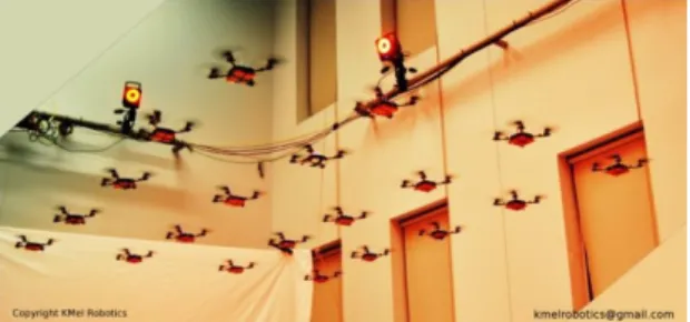
Figure 2.1: UAVs flying using a motion capture system for localization

2.2 VI-sensor

(8)

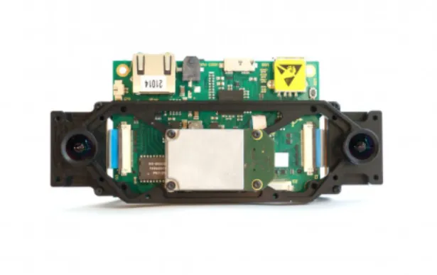
The VI-sensor comes with a factory calibration containing camera calibration and inter sensor dimensions. The base line of the stereo camera is 11 cm.

Figure 2.2: VI-sensor

2.3 EuRoC

This project is a follow-up of the EuRoC project at the University of Twente. The EuRoC project aimed at developing a platform for localization and mapping in an unknown environment with the help of two webcams and an IMU and lateron also a VI-sensor. An important recommendation from this project was to implement sensor fusion to increase the accuracy of the platform.

2.4 SLAM vs VO+IMU sensor fusion

Two approaches can be taken to solve the localization problem. The first solu-tion is Simultaneous Localizasolu-tion And Mapping (SLAM). The SLAM algorithm keeps track of the pose of the observer and of the pose of the recognized land-marks. The other solution is sensor fusion of Visual Odometry and an IMU. This approach only keeps track of the pose of the observer and not the landmarks. This makes that the pose estimation of the VO+IMU sensor fusion approach can drift over time since estimation errors are accumulating and can’t be cor-rected. The SLAM approach is not drifting since the drift of the observer can be observed by keeping track of the pose of the landmarks. A SLAM algorithm is therefore more complicated than a VO+IMU sensor fusion algorithm. SLAM also has a higher computational burden. The drift of the VO+IMU sensor fu-sion is not very big and can be corrected easily by the user. The disadvantage of the temporal drift does not weigh up to the advantage of easier implementation of the VO+IMU sensor fusion therefore this method will be chosen.

2.5 Visual odometry

(9)

1. Feature extraction 2. Feature matching 3. Motion estimation

The motion of the camera is calculated using only two consecutive frames so small errors in the estimation will accumulate and cause the estimate to drift. A pose estimation from visual odometry can be obtained by integrating the motion estimate. A comparison of different odometry methods for RGB-D cameras has been performed by Fang and Scherer[1]. They describe image based methods and depth based methods. Image based methods are found more faster and more accurate than depth based methods in feature rich environments. Since depth information from a stereo camera also relies on the number and quality of features it is better to look at the image based methods. Three image based methods are described of which only FOVIS[5] and VISO2[3] are applicable for monochrome stereo cameras. Both algorithms have a ROS implementation. The paper concludes that FOVIS is the best choice for accuracy and speed so FOVIS is chosen as visual odometry method.

2.6 Comparison of sensor fusion methods

The sensor fusion algorithm fuses visual odometry with IMU measurements. FOVIS provides a twist measurement including a covariance matrix. It can also provide a pose measurement which is the integration of the twist measurements. This pose measurement does not provide a covariance matrix. The IMU mea-surement consists of a linear acceleration and an angular velocity meamea-surement. Since we are not aiming at improving the state of the art we are looking for already implemented packages. This resulted in three packages: Robot pose EKF1, Robot localization2 and ETHZ ASL Sensor fusion3.

2.6.1 Comparison

Important properties of the sensor fusion is what it accepts as input measure-ment and which states are tracked. An overview of this can be seen in table2.1.

2.6.2 Remarks

Not everything can be put in a table so a few remarks on the different sensor fusion algorithms are made here.

2.6.2.1 Robot pose EKF

The sensor fusion algorithm uses only the orientation data provided in a ROS IMU message. This means that an extra filter is needed to estimate the orien-tation of the IMU based on the IMU measurements.

1_{http://wiki.ros.org/robot_pose_ekf}

2_{http://wiki.ros.org/robot_localization}

(10)

Robot pose EKF

Robot localization

ETHZ ASL Sensor fusion Input:

IMU _X* _X(multiple) _X(one) Pose sensor _X _X _X

Twist sensor _X Only linear velocity

Tracked states:

Position _X _X _X Linear velocity _X _X Linear acceleration _X _X Orientation _X _X _X Angular velocity _X _X

IMU bias _X

Sensor-IMU configuration _X

Pose scale _X

Roll and pitch drift _X

*Only accelerometer. Requires an extra filter to obtain attitude from IMU. Table 2.1: Overview of the inputs and the tracked states of the different sensor fusion algorithms

2.6.2.2 Robot localization

This sensor fusion is set up very general. It has an Extended Kalman Filter and an Unscented Kalman Filter implementation. The input measurements have to match the states such that the observation matrix H is identity. The process noise can be tuned by the user but it is not clear how this should be done.

2.6.2.3 ETHZ ASL Sensor fusion

This sensor fusion is designed for use with Micro Air Vehicles (MAV). It is based on an Extended Kalman Filter. The IMU is used in the propagation step. This makes that the linear acceleration and the angular velocity states can not be updated by other sensors than the IMU. The sensor fusion framework compensates for time delay in the measurements. The sensor-IMU configuration and the pose scale are also estimated but those are already known on beforehand. The process noise covariance is already determined in this implementation.

2.6.3 Choice of sensor fusion implementation

(11)

Chapter 3

Sensor fusion with

VI-sensor

This chapter details how the sensor fusion algorithm works. This sensor fusion algorithm is published by Weiss[12]. This sensor fusion algorithm has been implemented to work with the VI-sensor. The IMU measurements are fused with the pose estimation obtained by the visual odometry to obtain a high-bandwidth pose estimation from the VI-sensor. The sensor fusion is able to detect pitch and roll drift and can compensate for the time delay caused by the calculation time of the visual odometry. First the general functioning of the sensor fusion is elaborated. Then it will be described how the visual odometry pose has to be incorporated in the algorithm. The VI-sensor can also be used to create a map of the area. This will be described at the end of this chapter.

3.1 Software setup

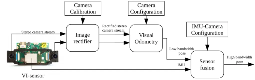
Figure 3.1shows the software setup which is used to obtain a high-bandwidth pose from the VI-sensor.

Figure 3.1: Software setup

(12)

calculate the pose using the rectified camera images and the known transfor-mation between both cameras. This pose is published at the frame rate of the camera which is 20 Hz in the case of the VI-sensor. The low bandwidth pose is fed to the sensor fusion together with the IMU data. The sensor fusion uses the known configuration of the IMU with respect to the camera to calculate a high bandwidth pose.

3.2 Sensor fusion

The sensor fusion algorithm used is an Error State Extended Kalman Filter (ESEKF) or Indirect Extended Kalman Filter. It uses three states: the true statexrepresenting the physical state in which the vehicle is, the estimated state

ˆ

x which is our estimation of the true state and the error state ˜x which is the difference between the true state and the error state˜x=x−ˆx. Ideally we want our estimated state to be the same as our true state so we want the error state to go to zero. The ESEKF measures the difference between our measurement and our estimation, which is the error, and uses this to calculate the corrections which has to be performed on the estimated state. This is elaborated more in the Kalman procedure. Recent work has been published which provides a very detailed description of the working of an ESEKF[10].

3.2.1 IMU as propagation sensor

The IMU is used as a propagation sensor in the sensor fusion. The bandwidth of the IMU is already high enough for the desired output bandwidth. Therefore it is unnecessary to compute extra prediction steps inbetween the IMU mea-surements. The IMU is affected by bias and noise. The bias is estimated in the filter and can therefore be compensated.

3.2.2 Coordinate frames

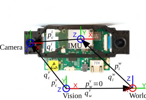
Four frames can be identified in the ESEKF model which can be seen in fig-ure3.2.

The world frame is always aligned with gravity. The IMU frame is the frame in which the IMU measurements are done. The camera frame is the origin of the reference camera. The vision frame is the world as observed by the cam-eras. The transformations between these frames are indicated using pand q.

pic describes the three-dimensional position of the origin of the camera frame of

reference expressed in the IMU frame of reference. qci is the quaternion

repre-sentation of the orientation of the camera frame of reference expressed in the IMU frame of reference. The same holds for the other transformations wherec

describes the camera frame of reference, v describes the vision frame of refer-ence, w describes the world frame of reference and i describes the IMU frame of reference.

(13)

Figure 3.2: Model used in EKF

initial rotation is incorporated in the rotation of the vision frame with respect to the world frame.

3.2.3 Drift observability

Since the pose measurements from visual odometry can drift the vision frame is defined separately from the world frame. The position drift of the visual odometry is unobservable in this setup. By forcing pv

w= 0 the position of the

vision frame equals the position of the world frame which means that the world frame is drifting in position along with the vision frame.

A drift in roll or pitch is observable using the gravity vector which can be obtained from the accelerometer. Therefore the rotation of the world frame in the vision frame can become non-zero. This non-zero rotation represents the roll and pitch drift of the visual odometry attitude measurement. A yaw drift is still unobservable. Therefore the yaw of the world frame is aligned with the yaw of the vision frame. This is done and further detailed in the update step of the ESEKF.

3.2.4 Kalman procedure

(14)

3.2.4.1 State vector

The state vector of the ESEKF is:

ˆ

x=pw_i vw_i q_iw bω ba λ qwv qic pic

T

(3.1) withpw_i and v_iw describing respectively the three-dimensional position and velocity and q_iw describing the quaternion representation of the orientation of the IMU frame expressed in the world frame. The three-dimensional vectors

bω and ba describe the bias terms on respectively the gyroscope and the

ac-celerometer. The scalar λ describes the scaling factor which is needed when scaled position measurements are done for example when using a mono camera setup. The quaternionqv

wdescribes the orientation of the world frame expressed

in the vision frame and the quaternionqi

c and the three-dimensional positionpic

describe respectively the orientation and the position of the camera expressed in the IMU frame.

The error state is defined as:

˜ x=p˜w

i v˜iw δθwi ˜bω ˜ba λ˜ δθwv δθic p˜ic

T

(3.2) where ˜pw_i represents the difference between the real position pw_i and the estimated position ˆpw_i: ˜pw_i =pw_i −pˆw_i. Similarly for velocity, scale and bias terms. The error in the orientation cannot be expressed by simple subtraction. The error in the orientation can be described by introducing the error quaternion:

δq_iw= ˆq_iw−1⊗q_iw (3.3) The ⊗ operator is the quaternion multiplication operator. This equation describes the same as:

δRw_i = ˆRw_i−1Rw_i (3.4) In the working area of the ESEKF the estimation of the orientation will be close to the real value of the estimation. This means that the error quaternion

δq is close to identity. This allows to use a small angle approximation of the error quaternion:

δRwi =I+bδθiwc× (3.5)

In which bxc× is the skew-symmetric matrix composed from the vectorx.

The relationship betweenδq andδθis given by:

δq≈

1 1₂δθx 12δθy 12δθz

T

=

1 1₂δθT

(15)

3.2.4.2 Propagation step

During the propagation step the states of the ESEKF are propagated using the IMU measurements. For every IMU measurement the following steps are performed:

1. Propagate the state variables according to their differential equations. For quaternions the first order quaternion integration is used[11].

2. Calculate Fd and Qd which describe the propagation of the error state

covariance matrix and the additional measurement noise.

3. Compute the propagated error state covariance matrix according to

Pk+1|k=FdPk|kFdT +Qd (3.7)

3.2.4.2.1 Propagate using differential equations

The differential equations used to propagate the state variables are: ˆ˙

pw_i = ˆv_iw

ˆ˙

vw_i =Rw_i (am−ˆba)−g

ˆ˙

qwi =

1

2Ω(ωm− ˆ

bω)ˆqwi

ˆ˙_b_ω_{= 0}_,ˆ˙_b_a _{= 0}_,ˆ˙_λ_{= 0} ˆ˙

p_ci = 0,qˆ˙i_c= 0,pˆ˙v_w= 0,qˆ˙v_w= 0

where am and ωm are respectively the measurements of the accelerometer

and the gyroscope and Ω(ω) is the quaternion-multiplication matrix ofω. It is constructed as:

Ω(ω) =



  

−ωx −ωy −ωz 0

0 ωz −ωy ωx

−ωz 0 ωx ωy

ωy −ωx 0 ωz



  

(3.8)

when the quaternion is defined asq=

qw qx qy qz

T

The position and velocity are updated according to

ˆ

pw_i

k+1|k = ˆp

w ik|k+ ˆ˙p

w i∆t

ˆ

viw_k₊₁|k = ˆv

w i_k|k+ ˆ˙v

w i ∆t

For the quaternion a first order quaternion integrator is used to integrate the quaternions[11].

3.2.4.2.2 Calculate propagation of error state covariance matrix and additional measurement noise

(16)

∆ ˙pw_i = ∆v_iw

∆ ˙v_iw=−Rw_ibam−bˆac×δθwi −R w

i ∆ba−Rwi na

δθ˙wi =−bωm−bˆωc×δθwi −∆bω−nω

∆˙bω=nbω ∆˙ba=nba ∆ ˙λ= 0

∆ ˙pi_c= 0 δq˙i_c= 0 ∆ ˙pv_w= 0 δq˙_wv = 0

The error state dynamics can be described in the linearized continuous time error state equation

˙˜

x=Fcx˜+Gcn (3.9)

with n being the noise vector n = nT

a, nTba, n

T ω, nTbω

T

. The continuous-time error state covariance matrixFc can be discretized:

Fd=exp(Fc∆t) =Id+Fc∆t+

1 2!F

2

c(∆t)

2

+. . . (3.10) A repetitive and sparse structure can be found in the matrix exponents which allows to expressFd exactly as

Fd =

       

I3 ∆t A B −Rˆwi

(∆t)2

2 03×13

03 I3 C D −Rˆwi ∆t 03×13

03 03 E F 03 03×13

03 03 03 I3 03 03×13

03 03 03 03 I3 03×13

013×3 013×3 013×3 013×3 013×3 I13         (3.11) with

A=−Rˆwi baˆc×

(∆t)2 2 −

(∆t)3

3! bωc×+ (∆t)4

4! (bωc×)

2

(3.12)

B=−Rˆw_i baˆc×

₋_(∆_t₎3

3! + (∆t)4

4! bωc×− (∆t)5

5! (bωc×)

2

(3.13)

C=−Rˆwi baˆc×

∆t−(∆t)

2

2 bωc×+ (∆t)3

3! (bωc×)

2

(3.14)

D=−A (3.15)

E=I3−∆tbωc×+

(∆t)2 2! (bωc×)

2 _(3.16) F =−∆t+(∆t)

2

2! bωc×− (∆t)3

3! (bωc×)

2 _(3.17)

(17)

Gc=        

03 03 03 03

−Rˆw

i 03 03 03

03 03 −I3 03

03 03 03 I3

03 I3 03 03

013×3 013×3 013×3 013×3         (3.18)

The discrete time system noise covariance matrixQd can now be calculated

as[6]:

Qd=

Z

∆t

Fd(τ)GcQcGTcFd(τ)Tdτ (3.19)

with

Qc=



  

σ2

na 03 03 03

03 σn2ba 03 03

03 03 σ2nω 03

03 03 03 σn2_bω



  

(3.20)

For the VI-sensor IMU, ADIS 16488, this matrix is

Qc=



  

0.0225632·I3 03 03 03

03 0.000082·I3 03 03

03 03 0.0042·I3 03

03 03 03 0.0000032·I3 

  

(3.21)

3.2.4.3 Measurement update

With only the propagation the error state covariance matrix will continue to grow i.e. the estimation becomes more uncertain. A measurement from another sensor can provide extra information to update the estimate and reduce the uncertainty. The Kalman procedure for the measurement update is as follows:

1. Compute the residual ˜z=z−zˆ

2. Compute the innovationS=HP HT +R

3. Compute the Kalman gain K=P HTS−1

4. Compute the correction ˆx˜=Kz˜

5. Update states ˆxk+1|k+1= ˆxk+1|k+ ˆx˜

6. Update error state covariance matrix

(18)

in whichz is the performed measurement, ˆz is the estimated measurement based on the estimated states,His the observation matrix relating the measure-ment error ˜z with the error state ˜xas ˜z =Hx˜. P is the error state covariance matrix andRis the measurement noise covariance matrix.

To process the measurement the residual ˜z, the observation matrix H and the measurement noise covariance matrix R have to be determined. The visual odometry pose is used as a measurement. This measurement can be split in three parts: the position, the attitude and an artificial yaw measurement. The artificial yaw measurement is included since the yaw drift is unobservable. By including an artificial yaw measurement it can be assured that the yaw of the vision frame is aligned with the yaw of the world frame. The three parts of the pose measurement can be computed separately and at the end combined in one observation matrix, one residual and one measurement noise covariance matrix.

3.2.4.3.1 Position measurement

For the position measurement the measurement function is:

hp(˜x) = ˜zp=Rvw(p w i +R

w i p

i

c)λ+np−Rˆvw(ˆp w i + ˆR

w i pˆ

i

c)ˆλ (3.22)

To obtain the observation matrix H the measurement function has to be linearized around the estimated state:

Hp=

∂hp(˜x)

∂x˜ |x=ˆx (3.23) This results in the following observation matrix:

Hp=

               ˆ Rv wλˆ

03x3

−RˆvwRˆiwbpˆ i c×cˆλ

03x3

ˆ

Rv

w(ˆpwi + ˆRwi pˆic)

−Rˆv_wb(ˆpw_i + ˆRw_i pˆi_c)ˆλ×c

03x3

ˆ

Rv wRˆwi ˆλ

               T (3.24)

How to derive this observation matrix is detailed in the appendix. The measurement noise covariance matrix was not given by the visual odometry so this is estimated at:

R=





0.01 0 0 0 0.01 0 0 0 0.01



 (3.25)

The residual is

˜

(19)

3.2.4.3.2 Attitude measurement

For the attitude measurement the measurement function is:

hq(˜x) = ˜zq = (ˆqcv)

−1_⊗_qv c = (ˆq

i c)

−1_⊗_(ˆ_qw i )

−1_⊗_(ˆ_qv w)

−1_⊗_qv w⊗q

w i ⊗q

i

c (3.27)

Linearizing this function around the estimated state results in the following observation matrix:

Hq =

              03x3 03x3 1 2R c i 03x3 03x3 0 1 2R c iRiw

1

2I3

03x3               T (3.28)

The measurement covariance matrixRis also not given for the attitude so it is also estimated. The estimation used is:

R=





0.02 0 0 0 0.02 0 0 0 0.02



 (3.29)

The residual of the attitude measurement is: ˜

zq = (ˆqcv)

−1_⊗_z

q (3.30)

3.2.4.3.3 Artificial yaw measurement

The artificial yaw measurement is to align the yaw of the vision frame with the yaw of the world frame. This can be achieved by using an observation scalar

H = 1, a measurement noise covariance of 1·10−6 and a residual

y=yaw((ˆqwv)−

1

⊗qvw) (3.31)

where the yaw of a quaternion is calculated as

yaw(q) =atan2(2(qwqz+qxqy),(1−2(q2y+q

2

z))) (3.32)

3.2.4.4 Complete measurement

The three parts can be combined together. This will result for the observation matrix in   ˜ zp ˜ zq ˜ zyaw  =   Hp Hq 1 

(20)

The total measurement error covariance matrix is R=          

0.01 0 0 0 0 0 0 0 0.01 0 0 0 0 0 0 0 0.01 0 0 0 0 0 0 0 0.02 0 0 0 0 0 0 0 0.02 0 0 0 0 0 0 0 0.02 0 0 0 0 0 0 0 1·10−6

          (3.34)

And the total residual is

˜

z=





zp−Rˆvw(ˆpiw+ ˆRwipˆic)ˆλ

(ˆqv

c)−1⊗zq

yaw((ˆq_wv)−1⊗qv_w)



 (3.35)

3.2.5 Fixed and known configuration

The EKF was designed for configurations in which the scale and the camera-IMU configuration is not known on beforehand. That means that those values are incorporated in the state vector. In our configuration however the camera-IMU configuration is known since the stereo cameras were calibrated in the factory and this data is provided with the cameras. Also the scale is known and fixed on 1 since a stereo camera is used. The states pi

c, δθic and λcould be removed

from the state vector since their values do not need to be estimated. But the software implementation also allows to fix the scale and the configuration. In addition the initial error state covariance matrix has to be put to zero at the rows and columns corresponding to the known states. This makes the filter know that these states are fully known.

3.2.6 Lost visual odometry

It can happen that the visual odometry algorithm is not able to estimate the pose. This can be caused for example when it can’t find enough features in the image. The algorithm will produce a faulty measurement which can be recog-nized by all zeros. In such a situation the measurement should not be taken into account in the sensor fusion. This can be done by setting the H-matrix and the residual to zero. The state estimation of the sensor fusion will now only be determined based on the IMU.

When the visual odometry has recovered it will continue to provide measure-ment data. The motion estimation is again valid but the pose estimation, which is an integration of the motion estimation, will continue from the pose it had before the visual odometry was lost. This is not correct. It should start from the pose estimation given by the sensor fusion at the moment of recovery. This error can be compensated by introducing a bias on the pose. This bias will be calculated at the moment of recovery.

(21)

Where ˆz is the expected measurement value using the estimated states of the sensor fusion andzis the obtained measurement value. The calculated bias should now be added to every new measurement value.

zp=pbias+zp

zq =qbias⊗zq

Next to an update of the measurement using a bias term the uncertainty of the measurement value has also increased.

3.2.7 Time delay compensation

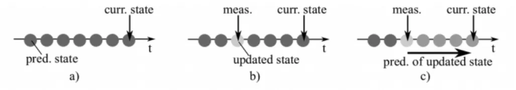
A useful property of the ESEKF implementation of Weiss[12] is that it allows for time delay compensation. The visual odometry algorithm which extracts the pose from the camera images takes some time and meanwhile the IMU has already propagated further. Timestamps of the camera images and the IMU are used to update the ESEKF at the time where the measurement took place. Then the state is further propagated from the time where the measurement took place using buffered IMU-measurements. This is shown in figure3.3.

Figure 3.3: Time delay compensation in the ESEKF

In a) the UAV is using the current state as reference. In b) a delayed mea-surement update arrives and the corresponding buffered state is corrected using the measurement. In c) the states following the corrected states are corrected by propagating the buffered IMU measurements using the propagation step of the ESEKF.

3.3 Mapping

(22)

Chapter 4

Realisation

Chapter 3 showed the theoretical approach toward the use of the VI-sensor as a high bandwidth pose sensor. The next step is to set up a system in which the external pose estimation can be used to control a UAV. This chapter first describes how the UAV is setup. Then the setup used to control the UAV is elaborated. Since the first test flights are performed inside an OptiTrack area a fail-safe has been implemented which switches back to OptiTrack in case visual odometry fails. This will described in the end of this chapter.

4.1 System setup

The UAV used is the ArduCopter Hexa-B. Six AC2830-358 850Kv motors are mounted on the frame. The ESCs are from 3D Robotics and can deliver 20 A of current and 6-16.8 V DC voltage. A FPV Radio Telemetry Ground Module is also mounted which allows wireless Mavlink communication. The flight con-troller used is a Pixhawk.

(23)

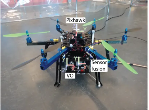
Figure 4.1: Hexacopter

The picture shows the UAV. On top and in the center of the UAV the Pix-hawk flight controller is located. The grey balls are the OptiTrack markers used for the OptiTrack pose estimation. The blue arms of the UAV show the front of the UAV. At the front the VI-sensor is mounted. At the back the Intel NUC is mounted. Both units weigh approximately the same and are placed such that the center of mass of the UAV stays in the center of the UAV.

In this picture also relevant frames are shown. The visual odometry (VO) frame is located in the reference camera and is the frame in which the visual odometry algorithm expresses its pose. The sensor fusion frame is located in the IMU of the VI-sensor and is the frame in which the sensor fusion expresses its pose. The Pixhawk frame is located in the IMU of the Pixhawk and is the frame in which the Pixhawk expresses its pose. Based on this pose the UAV is controlled. The OptiTrack pose is not shown for clarity of the image but the frame is in approximately the same position and orientation as the Pixhawk frame.

4.2 Control setup

(24)

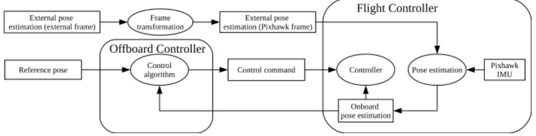
Figure 4.2: Control setup

Two external poses can be seen in figure 4.2. One is the external pose expressed in its own frame. The location of these frames can be seen in figure4.1. The other is the external pose expressed in the Pixhawk frame. Inbetween is a transformation which transforms the external pose from its own frame to the Pixhawk frame. This external pose can be OptiTrack, visual odometry, the pose output of the sensor fusion or another pose. In the Pixhawk the external pose is used in the pose estimation to compensate for drift of the Pixhawk IMU. The onboard pose estimation consists of two parts: an attitude estimation and a position estimation. Both estimators estimate position and attitude based on IMU readings from the Pixhawk IMU which are corrected by the external pose. The onboard pose estimator publishes its pose which is used in the offboard controller. The control algorithm compares the onboard pose estimation with a reference pose and publishes a control command based on this difference. This control command is sent to the controller onboard the Pixhawk.

4.2.1 Frame transformation

Figure4.2shows that a frame transformation is required to transform the pose expressed in the external frame such that it is expressed in the Pixhawk frame. For the visual odometry and the sensor fusion this pose is estimated using a ruler. The position of the VO frame expressed in the Pixhawk frame is estimated at

pP_{V O}=





0.15

−0.055

−0.1



 (4.1)

The rotation of the VO frame expressed in the Pixhawk frame is estimated at

RP_{V O}=





0 0 1 1 0 0 0 1 0



 (4.2)

For the sensor fusion the rotation is estimated the same as VO RP

SF =RPV O.

The position is estimated at

pP_SF =





0.15 0

−0.1



 (4.3)

(25)

posi-Pixhawk frame aligned with the OptiTrack frame. This makes that no transfor-mation matrix is required since the OptiTrack frame is aligned in position and orientation with the Pixhawk frame.

4.2.2 Offboard controller

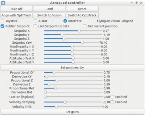
The offboard controller used is a PD position+yaw controller with velocity set-points as a control command to the Pixhawk. Velocity setset-points as an output is chosen because of compatibility with other UAVs. Also an advantage of using an offboard control algorithm is that it is easier to tune and understand what is going on. The reference position and yaw can be set by a Graphical User Inter-face (GUI). This GUI also allows to set the gains of the controller. A screenshot of the GUI can be seen in figure4.3.

Figure 4.3: Graphical User Interface

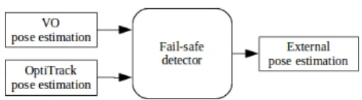
4.3 Fail-safe

(26)

Figure 4.4: Fail-safe

The input poses are not aligned with each other. For continuity in the output of the fail-safe during the switch it is necessary that both poses are aligned with each other. The OptiTrack pose is sent as the external pose when the fail-safe is activated. For fail-safety it is best that the OptiTrack pose is not changed. Therefor the VO pose has to modified to align both input poses. How to align these frames is elaborated in subsection 4.3.1. With the input poses aligned the fail-safe also has to decide whether it should be activated. This is further elaborated in subsection 4.3.2.

4.3.1 Frame alignment

The vision pose and the OptiTrack pose are not aligned with each other. Both poses are presented in their own frame of reference. The vision pose can be expressed as homogeneous matrix HV

S. A homogeneous matrix describes the

orientation and translation in one matrix:

HSV =

RV

S p

V S

0 1

(4.4) whereRV_S is the orientation of the sensor expressed in the visual odometry frame of reference andpV_S is the position of the sensor expressed in the VO frame of reference. In the same way the OptiTrack pose can be expressed asH_SO which is the pose of the sensor expressed in the OptiTrack reference frame.

The OptiTrack frame is used as reference frame so the sensor pose expressed in the VO frame has to be expressed in the OptiTrack reference frame. To express the sensor pose in the OptiTrack reference frame the following transformation is needed:

H_SO=H_VOH_SV (4.5) This requires the transformation matrixHO

V. This transformation matrix

can be calculated during a frame alignment procedure:

H_SO=H_VOH_SV (4.6)

(27)

used. Aligning the OptiTrack reference frame with the VO reference frame would require to transform the OptiTrack pose which is not desirable since the OptiTrack is the backup and transforming this pose might cause the backup to fail.

4.3.2 Switching procedure

There are two situations in which the fail-safe should switch to OptiTrack. The most obvious one is when the visual odometry fails to estimate a pose. This can be caused by insufficient inliers or a reprojection error. This is easy to detect since an error is produced by the VO algorithm. The other situation is when the visual odometry provides a bad estimation which is way off the actual value. This can happen when the visual odometry has little features but still finds a solution (which is an incorrect solution). To detect this situation the velocity of the visual odometry is compared with the velocity of the OptiTrack pose measurement. When the difference exceeds a threshold value, the fail-safe switch is activated. The velocity of the VO can be obtained directly from the velocity measurement of the VO. For OptiTrack only a pose measurement is received. To estimate the OptiTrack velocity a first order fixed window approach is used with a window of 10 samples. This calculates the velocity as

v(n) =p(n)−p(n−10)

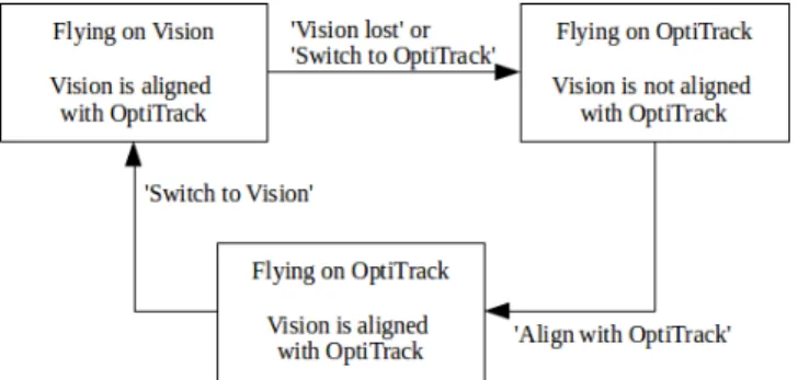
t(n)−t(n−10) (4.8) The fail-safe detector has been implemented as a state machine. This can be seen in figure 4.5.

Figure 4.5: Fail-safe detector state machine

(28)

(29)

Chapter 5

Experiments and discussion

Three experiments have been performed to test the performance of the algo-rithms presented before. The first experiment compares the different position and yaw estimation algorithms during a flight. It appeared that motor vi-brations affect the sensor fusion a lot therefore a second experiment has been performed in which the motors are not armed. The third experiment shows the results of the mapping algorithm described in chapter 2. At the end of the chapter there is a discussion on the experiments and the presented work.

5.1 Evaluation of position and yaw estimation

during flight

The goal of this experiment is to evaluate and compare the position and yaw estimations of the different pose estimation algorithms. The experiment setup is shown in figure 5.1.

Figure 5.1: Experiment setup

(30)

The other path in the figure shows the VO pose fused with the VI-sensor IMU using the ESEKF. This results in the sensor fusion pose expressed in the sensor fusion frame. Unfortunately the frame transformation to express the pose in the Pixhawk frame is forgotten to include here. The sensor fusion pose is also aligned with the OptiTrack pose such that the poses are easy to compare. This results in the sensor fusion pose expressed in the sensor fusion frame aligned with OptiTrack. The position and yaw of the pose estimations in the grey boxes are compared in the experiments.

The motor vibrations have a big effect on the IMU measurements. This is shown in figure 5.2

Figure 5.2: Effect of motor vibrations on IMU measurements

The noise on the accelerometer and gyroscope increases a lot when the mo-tors are armed at around t = 8. This effect will be taken into account in the sensor fusion by increasing the noise parameters of the accelerometer and the gyroscope by a factor 100. The bias parameters remain the same.

(31)

Figure 5.3: Comparison of pose estimation algorithms, x and y.

(32)

It can be seen that the UAV follows the setpoint. How well it follows this setpoint is a matter of control. In this experiment we are only interested in the accuracy of the pose estimation. It can be seen that for x, y and z the VO, the Pixhawk and the OptiTrack estimations are similar. Forxandzthe Sensor fusion estimation clearly shows a low accuracy. Foryhowever it seems to follow the OptiTrack estimation. A remark has to be made for the Sensor fusion. The frame transformation shown in figure4.2has not been included. The alignment procedure compensates for this error when the yaw does not change but at

t = 40−48 the yaw changes which causes an error inx and y at that time. The yaw estimation of OptiTrack shows short peaks. OptiTrack estimates the pose based on the location of multiple markers. If these markers are close to a rotation-symmetric configuration OptiTrack can measure a different orientation of the UAV. This could be the cause of these short peaks. In these figures it is hard to see what the differences between the different pose estimation algorithms are. In figure 5.5 and figure5.6 these differences are better shown. In these figures OptiTrack is used as ground truth and for every pose estimation the difference with OptiTrack is shown. The absolute position error in figure5.6

is calculated by ep=

q e2

x+e2y+e2z.

(33)

Figure 5.6: Pose estimation error for yaw and absolute position error. Figure5.5shows that the error of the VO position is within 3 cm forxand within 6 cm for y. The position error in z shows a drift of approximately 13 cm after 60 seconds. The absolute position error shown in figure 5.6 is also approximately 13 cm which is mostly caused by the position error inz. For the error in yaw it can be seen that the error stays within 3 degrees. It was expected that the Pixhawk error would follow the VO error but apparently they are not the same. It is not clear what the reason is why they are not the same.

5.2 Evaluation of sensor fusion

(34)

Figure 5.7: Evaluation of sensor fusion, x and y.

(35)

In this figure it can also be seen that an extra error in the sensor fusion positionxandyis introduced when the UAV is yawing fromt= 35−42. Around

t = 25 a short OptiTrack error occurred. Since the fail-safe algorithm checks the difference in velocity of OptiTrack and VO the fail-safe is also activated when OptiTrack generates a position error. That is the case at around t= 25. From this moment the Pixhawk pose estimation receives OptiTrack as external pose. The peaks in the yaw plot have the same reason as with the previous experiment. In these figures the performance of the sensor fusion is better now. Still it is hard to see how well it is performing. Therefore also an error plot is made. This can be seen in figure5.9and figure5.10.

(36)

Figure 5.10: Evaluation of sensor fusion for yaw and absolute position error. Still the error due to the missing transformation matrix can be seen. Apart from that the sensor fusion seems to follow the VO. The absolute position error is approximately 25 cm after 50 seconds but then reduces to approximately 15 cm.

5.3 Mapping

(37)

Figure 5.11: Octomap of the small fly arena of the RAM group at the University of Twente

Figure 5.12: Comparison of map and photo.

The comparison of the map and the photo shows that walls closeby are well observed. Also the glass door can be seen in the map as a rectangular hole in the wall. Below in the image also the desk with the computer can be observed. Further away from the UAV the map does not look that accurate anymore. This could be caused by the Stereo Block matching algorithm not being accurate at long distances. Maybe other point cloud generation techniques will provide better results.

5.4 Discussion

This section will discuss the experimental results and the presented work.

5.4.1 Frame transformation

(38)

The experiments shown in section5.1and5.2show that not incorporating this transformation leads to additional errors. For VO this transformation between VO and Pixhawk has been estimated using a ruler and for OptiTrack it is tried to align the OptiTrack frame as good as possible with the Pixhawk frame such that no transformation is needed. The better this transformation is estimated, the lower the error caused by misalignment will affect the pose estimation. This would result in better flight performance. The sensor fusion described in chapter 3 is able to estimate the transformation matrix between an external pose sensor and an IMU. This could be used to estimate these frame transformations.

5.4.2 Motor vibrations

As shown in figure5.2the motor vibrations have a big effect on the IMU mea-surements of the VI-sensor IMU. The experiments show that this deteriorates the performance of the sensor fusion. Already damping between the UAV and the VI-sensor has been applied to reduce the vibrations but this is still not enough. Aligning the motors could help to reduce the vibrations of the motor. The motor vibrations are now tried to be compensated by modeling it as an increase of noise in the sensor fusion. However, the source of the vibrations is clear and since the motors are spinning at high speed the vibrations could also be reduced by applying a low-pass filter on the IMU measurements. This has been researched a little bit with Matlab on the same IMU data as figure 5.2. An averaging filter where the last five measurements are averaged gives the following result:

(39)

It can be seen that the vibrations are reduced significantly compared to figure5.2. But this has to be tested to evaluate the effects in the real setup.

5.4.3 Sensor fusion

The ESEKF is implemented to obtain a high-bandwidth pose estimation from the VI-sensor. This is useful when the VI-sensor is used separately. However in the UAV setup also a sensor fusion algorithm is implemented onboard of the UAV. This made it possible to fly the UAV using only the VO measurement. The proposed setup had two sensor fusion algorithms cascaded. When the sensor fusion performs properly with the motors armed it should be tested if this cascaded sensor fusion will have better performance than using only one sensor fusion algorithm. Bypassing the Pixhawk sensor fusion however requires that the control of the UAV also has to be done offboard.

5.4.4 VO-IMU coupling

The visual odometry pose estimation and the IMU are loosely-coupled in the ESEKF meaning that both are treated as separate parts not interacting with each other. This makes that when visual odometry is lost it re-initializes from its last known visual odometry pose and not the sensor fusion pose. An attempt has been done to re-initialize at the sensor fusion pose but this hasn’t been tested. It may be better to use a tightly-coupled sensor fusion for fusing the visual odometry pose with the IMU.

5.4.5 Point cloud generation

The map is generated based on the point clouds which are generated from the stereo camera images. The algorithm used for this is Stereo Block matching. According to the KITTI benchmark[7] there are algorithms with better results which can also run at real time. A more accurate point cloud results in a more accurate map.

5.4.6 Outdoor

The setup has now only been tested indoor. It is designed for outdoor operation so additional experiments should be performed to test the performance in an outdoor environment.

5.4.7 Multiple sensors

(40)

Chapter 6

Conclusion and

recommendations

6.1 Conclusion

This project aimed at obtaining an accurate localization from vision. The VI-sensor was used to provide stereo camera images and IMU measurements. The visual odometry algorithm FOVIS obtained a pose estimation from the stereo camera images. The sensor fusion algorithm published by Weiss has been used to fuse the VO pose with the IMU measurements. This provides a high-bandwidth pose estimation from the VI-sensor. This high-bandwidth pose estimation was aimed to be used in a UAV setup providing the localization of the UAV. How-ever the motor vibrations affected the sensor fusion too much to be used in the setup. Therefore only the low-bandwidth VO pose has been used for providing the localization of the UAV. A working setup has been created with a hexacopter equipped with the VI-sensor and an Intel NUC which can fly using visual odom-etry pose estimation. A fail-safe has been designed and implemented to prevent the UAV from crashing when visual odometry fails and flying inside an Opti-Track area. Experiments show a good accuracy and drifts up to 15 cm/min. During the flight also a map of the environment can be created.

6.2 Recommendations

6.2.1 Robust pose from vision

(41)

6.2.2 Motor vibrations

The effect of motor vibrations on the IMU measurements has to be reduced. This should be done preferably mechanically. Using proper damping between the motors and the VI-sensor can reduce the damping. This has to be investi-gated more. Another mechanical solution is aligning the motors to reduce the eccentricity. The effect of vibrations can also be reduced in the software by implementing a low-pass filter on the IMU measurements.

6.2.3 Frame transformation estimation

Using incorrect frame transformations between the Pixhawk and the external pose sensor leads to additional errors in the localization. These frames have to be estimated more accurately. The sensor fusion algorithm of Weiss described in this project can likely be used to estimate these frame transformations.

6.2.4 Cascaded sensor fusion

When the ESEKF provides accurate enough pose estimations to be used in flight the system consists of two sensor fusion algorithms: the ESEKF and the onboard pose estimation. It should be investigated how much benefit is gained from using only VO and onboard pose estimation to using ESEKF and onboard pose estimation.

6.2.5 Outdoor testing

The setup has been designed for outdoor operation but it has never been tested outdoor. This should be done to verify that the setup can be used outdoor.

6.2.6 Additional sensors

More sensors should be added to reduce the dependency on the visual odometry pose. When VO is lost this shouldn’t lead to uncontrollability of the UAV. For example including GPS would still provide pose estimation when VO is lost even if this GPS pose is less accurate. It should be considered however that extra sensors will add extra mass to the UAV.

6.2.7 SLAM

(42)

6.2.8 Multi sensor fusion

In this project the single sensor fusion (SSF) framework has been used. From the same authors and with the same principle also exists the multi sensor fusion (MSF) framework. This allows to fuse more than one sensor with the IMU measurements. Also when only one sensor is used next to the IMU it is good to use the MSF since it seems that this framework is maintained.

6.2.9 Point cloud generation

The map is built using point clouds generated by Stereo Block Matching. As shown in the discussion better point cloud generation techniques exist. Imple-menting these newer techniques would increase the accuracy of the generated point cloud and therefore also the accuracy of the created map.

6.2.10 VIKI integration

VIKI is a ROS GUI currently developed within the AEROWORKS group. Its goal is to make it easier for the user to use ROS packages and connecting different packages into one system. This requires a modular design of the system. The current implementation of this project has to be made more modular. The fail-safe, control and GUI are now integrated in one module while it would be better to separate these modules. Then the modules have to be integrated in the VIKI framework.

6.2.11 Haptic interface

(43)

Appendix A

Observation matrix of

ESEKF

This appendix describes how to derive the observation matrix used in the ES-EKF. The observation matrixH relates the measurement function ˜zto the error state used in the ESEKF ˜xas

˜

z=Hx˜ (A.1)

A.1 Position

For the position measurement part the following measurement function is used:

hp(˜x) = ˜zp=Rvw(p w i +R

w ip

i

w ipˆ

i

c)ˆλ (A.2)

To obtain the observation matrix, this function has to be linearized around the estimated state:

Hp=

∂hp(˜x)

∂x˜ |x=ˆx (A.3) This equation can be solved for every state apart and then be concatenated at the end. Let’s start with solving it for ˜pw

i. First we fill in the equation:

∂hp(˜x)

∂p˜w i

|x=ˆx=

∂(Rv_w(pw_i +Rw_i pi_c)λ+np−Rˆvw(ˆp w i + ˆR

w i pˆ

i c)ˆλ)

∂p˜w i

|x=ˆx (A.4)

We want to find the derivative with respect to ˜pw

i . It can be seen that pwi

can be rewritten aspw

i = ˜pwi + ˆpwi . This will result in the following equation:

∂hp(˜x)

∂p˜w i

|x=ˆx=

∂(Rv

w((˜pwi + ˆpwi) +Rwi pic)λ+np−Rˆwv(ˆpwi + ˆRwi pˆic)ˆλ)

∂p˜w i

|x=ˆx

(44)

∂hp(˜x)

∂p˜w i

|x=ˆx=

∂( ˆRv

w((˜pwi + ˆpwi) + ˆRwipˆic)ˆλ+np−Rˆwv(ˆpwi + ˆRwipˆic)ˆλ)

∂p˜w i

(A.6) Analysing this equation shows that a lot of variables are cancelled out. Re-moving this variables will result in:

∂hp(˜x)

∂p˜w i

|x=ˆx=

∂( ˆRv

wp˜wiλˆ+np)

∂p˜w i

(A.7) Since ˆλis a scalar it is easy to solve the equation now resulting in

∂hp(˜x)

∂p˜w i

|x=xˆ= ˆRvwλˆ (A.8)

The same procedure can be repeated for the other states. For calculating

∂h(˜x)

∂v˜w i

|x=xˆit is easy to see that

∂hp(˜x)

∂v˜w i

|x=ˆx=

∂(Rvw(pwi +R w i p

i

c)λ+np−Rˆvw(ˆpwi + ˆR w i pˆ

i c)ˆλ)

∂v˜w i

|x=ˆx (A.9)

=03x3 (A.10)

For determining the derivative with respect toδθw

i the derivation is slightly

different. We first start with writing down the equation

∂hp(˜x)

∂δθw i

|x=xˆ=

∂(Rv

w(pwi +Rwi pic)λ+np−Rˆvw(ˆpwi + ˆRwi pˆic)ˆλ)

∂δθw i

|x=ˆx (A.11)

Now we want to substituteRw

i with a term containing the estimate ˆRwi and

the error δθw

i . This relation can be derived from the definition of the error

quaternion.

q_iw= ˆq_iw⊗δq_iw (A.12)

Rw_i =R_ˆw_i Rˆi_i (A.13) = ˆRw_i (I3+bδθiw×c) (A.14)

This relation can now be used to substituteRw i .

∂hp(˜x)

∂δθw i

|x=ˆx=

∂(Rv_w(pw_i + ˆR_iw(I3+bδθiw×c)p i

w ipˆ

i c)ˆλ)

∂δθw i

|x=ˆx

(A.15) From here the same procedure is used by evaluating the equation atx= ˆx

(45)

∂hp(˜x)

∂δθw i

|x=ˆx=

∂( ˆRv

w(ˆpwi + ˆRwi (I3+bδθwi ×c)ˆpic)ˆλ+np−Rˆvw(ˆpiw+ ˆRwi pˆic)ˆλ)

∂δθw i

(A.16) = ∂( ˆR

v

wRˆwibδθiw×cpˆicλˆ+np)

∂δθw i

(A.17) The final step is to rewrite the equation such thatδθw_i is moved to the end of the equation. This can be done by using the relation

A×B=−B×A (A.18) When this is applied on the equation this would make

bδθ_iw×cpˆi_c=−bpˆi_c×cδθ_iw (A.19) This will continue the derivation with

∂hp(˜x)

∂δθw i

|x=ˆx=

∂( ˆRv_wRˆw_i bδθ_iw×cpˆi_cˆλ+np)

∂δθw i

(A.20) =∂(−

ˆ

RvwRˆwi bpˆ i

c×cδθiwλˆ+np)

∂δθw i

(A.21) =−Rˆ_wvRˆ_iwbpˆi_c×cˆλ (A.22) The derivation of the other states is similar to the derivations described above. The derivations are listed below.

The derivative with respect to ˜bω:

∂hp(˜x)

∂˜bω

|x=xˆ=

∂(Rv

∂˜bω

|x=ˆx

=03x3

The derivative with respect to ˜ba:

∂hp(˜x)

∂˜ba

|x=xˆ=

∂(Rv

∂˜ba

|x=ˆx

=03x3

(46)

∂hp(˜x)

∂˜λ |x=ˆx= ∂(Rv

∂˜λ |x=ˆx

= ∂(R

v

w(pwi +R w i p

i

c)(˜λ+ ˆλ) +np−Rˆvw(ˆpwi + ˆR w i pˆ

i c)ˆλ)

∂λ˜ |x=xˆ

= ∂( ˆR

v

w(ˆpwi + ˆRwi pˆic)(˜λ+ ˆλ) +np−Rˆvw(ˆpwi + ˆRiwpˆic)ˆλ)

∂λ˜

= ∂( ˆR

v

w(ˆpwi + ˆRwi pˆic)˜λ+np

∂˜λ

= ˆRv_w(ˆpw_i + ˆRw_ipˆi_c) The derivative with respect toδθv w:

∂hp(˜x)

∂δθv w

|x=ˆx=

∂(Rv

w(pwi +Rwipic)λ+np−Rˆwv(ˆpwi + ˆRiwpˆic)ˆλ)

∂δθv w

|x=xˆ

=∂( ˆR

v

w(I3+bδθvw×c)(pwi +Rwi pic)λ+np−Rˆvw(ˆpwi + ˆRwi pˆic)ˆλ)

∂δθv w

|x=ˆx

=∂( ˆR

v

w(I3+bδθvw×c)(ˆpwi + ˆR w i pˆ

i

c)ˆλ+np−Rˆvw(ˆpwi + ˆR w i pˆ

i c)ˆλ)

∂δθv w

=∂( ˆR

v

wbδθvw×c(ˆpwi + ˆRwi pˆic)ˆλ+np)

∂δθv w

=∂(−Rˆ

v

wb(ˆpwi + ˆRwi pˆic)ˆλ×cδθwv +np)

∂δθv w

=−Rˆwvb(ˆpwi + ˆRiwpˆic)ˆλ×c

The derivative with respect toδθi c:

∂hp(˜x)

∂δθi c

|x=xˆ=

∂(Rv

∂δθi c

|x=ˆx

=03x3

The derivative with respect to ˜pic:

∂hp(˜x)

∂p˜i c

|x=ˆx=

∂(Rv

w(pwi +Riwpic)λ+np−Rˆwv(ˆpwi + ˆRiwpˆic)ˆλ)

∂p˜i c

|x=xˆ

=∂(R

v

w(pwi +R w i (˜p

i

c+ ˆpic))λ+np−Rˆvw(ˆpwi + ˆR w i pˆ

i c)ˆλ)

∂p˜i c

|x=ˆx

=∂( ˆR

v

w(ˆpwi + ˆRiw(˜pic+ ˆpic))ˆλ+np−Rˆvw(ˆpwi + ˆRwi pˆic)ˆλ)

∂p˜i c

=∂( ˆR

v

w(ˆpwi + ˆRiwp˜ic)ˆλ+np)

(47)

This will result in the following observation matrix:

Hp=

               ˆ Rv wˆλ

03x3

−Rˆv_wRˆ_iwbpˆi_c×cλˆ

03x3

ˆ

Rv

w(ˆpwi + ˆRwi pˆic)

−Rˆv

wb(ˆpwi + ˆRiwpˆic)ˆλ×c

03x3

ˆ

RvwRˆwiλˆ

               (A.23)

A.2 Attitude

For the position measurement part the following measurement function is used:

hq(˜x) = ˜zq= (ˆqvc)−1⊗qvc = (ˆqci)−1⊗(ˆqwi )−1⊗(ˆqwv)−1⊗qvw⊗qwi ⊗qic (A.24)

To obtain the observation matrix, this function has to be linearized around the estimated state:

Hq =

∂hq(˜x)

∂x˜ |x=ˆx (A.25) This derivation can also be split up in three parts containing. The first part is the derivative with respect to δθi

c. The derivative is calculated atx= ˆxso

every quaternion exceptqi

c can be substituted by its estimated variant:

hq(˜x) = (ˆqci)

−1_⊗_(ˆ_qw i )

−1_⊗_(ˆ_qv w)

−1_⊗_q_ˆv w⊗qˆ

w i ⊗q

i

c (A.26)

The equation ˆq−1_⊗_q_ˆ_{results in the unit quaternion and can then be removed}

from the equation. This results in the following equation:

hq(x˜) = (ˆqci)−1⊗qic (A.27)

This equation can be recognized as the definition of the error quaternion so it can also be written as

hq(˜x) =δqic (A.28)

The error quaternion can also be written as its small angle approximation:

hq(x˜) =

1 1 2δθ i c (A.29) When we now look at the derivative ∂hq(˜x)

∂δθi c

it can be solved as

∂hq(˜x)

∂δθi c

=1

2I3 (A.30) Forδθw

(48)

hq(˜x) = (ˆqci)

−1_⊗_(ˆ_qw i )

−1_⊗_(ˆ_qv w)

−1_⊗_q_ˆv w⊗q

w i ⊗qˆ

i c

= (ˆqci)−

1

⊗(ˆqwi )−

1

⊗qwi ⊗qˆ i c

= (ˆq_ci)−1⊗δq_iw⊗qˆ_ci

Now we need the following quaternion property:

q⊗

0

x

⊗q−1=

0

Rx

(A.31) whereqandR describe the same rotation.

Now the equation can be rewritten as

hq(˜x) =

1 0 0 Rc

i

δqwi

=

1 0 0 Rc

i 1 1 2δθ w i

The partial derivative can now be solved:

∂h(x˜)

∂δθw i

= ∂(R

c i12δθ

w i ) ∂δθw i = 1 2R c i

And last forδθvwthe same procedure can be followed to find the solution:

h(˜x) = (ˆqv_c)−1⊗q_cv= (ˆq_ci)−1⊗(ˆq_iw)−1⊗(ˆqv_w)−1⊗q_wv ⊗qˆw_i ⊗qˆ_ci = (ˆqi_c)−1⊗(ˆqw_i )−1⊗δθ_wv ⊗qˆw_i ⊗qˆi_c

=

1 0 0 Rc_i

1 0 0 Riw

δq_wv

=

1 0 0 Rc_i

1 0 0 Riw

1 1 2δθ v w

∂h(˜x)

∂δθv w

=∂(R

c iR

i w12δθ

v w) ∂δθv w =1 2R c iR i w

This makes the full observation matrix

Hq =

              03x3 03x3 1 2R c i 03x3 03x3 0 1 2R c iRiw

(49)

Appendix B

Physical design

The hexacopter was already assembled and available. A few mounts have been made for the Pixhawk, VI-sensor and Intel NUC.

B.1 Mount of VI-sensor and NUC

Mounting the VI-sensor and the Intel NUC required some more effort. The first designs which were made were passing too much vibrations of the motors to the IMU of the VI-sensor. A few iterations have been made to end up with the design presented in figureB.1.

(50)

On the left side of the image the VI-sensor can be recognized and on the right side the Intel NUC can be recognized. The VI-sensor is put at the front of the UAV. The mount is connected to the UAV with the four blue dampers. These dampers reduce the vibrations of the motors on the mount.

B.2 Electronics

A few components on the UAV need to be powered. That is the Pixhawk, the VI-sensor, the Intel NUC and the motors. The Pixhawk came with its own power module which ensured correct powering of the Pixhawk. The following table lists the voltage specifications of the different components.

Component Voltage

VI-sensor 10-13 V Intel NUC 12-19 V Motors 6-16.8 V

The system is powered by a LiPo battery. The LiPo battery is a series of LiPo cells which determine the voltage. The following table lists the voltage provided by different LiPo batteries.

Number of cells Minimum voltage Maximum voltage

1S 3.2 4.2 2S 6.4 8.4 3S 9.6 12.6 4S 12.8 16.8

5S 16 21

It can be seen that the Intel NUC requires a 4S battery, the motors can operate with a 2S, 3S or 4S battery. The VI-sensor requires a 3S battery. A 4S battery is chosen as power source. A voltage regulator is used to provide the correct voltage for the VI-sensor. The circuit of the voltage divider can be seen in figureB.2.

Figure B.2: Voltage regulator

(51)

avail-Appendix C

Software setup

This appendix will elaborate the implementation of the software structure. A block diagram of the software setup is given in figure C.1. Different colors are used to distinguish the different elements of the software. The blue color rep-resents the visual odometry. The red color reprep-resents the mapping. The green color represents the sensor fusion. The purple color represents the Pixhawk pose estimation. The yellow color represents the control algorithms and the grey color represents OptiTrack. How this software structure is implemented in ROS is given in figure C.2. The ellipses represent nodes and the rectangles represent topics. In the rest of this appendix every ROS node will be explained.

C.1 vi sensor node

The package vi_sensor_node interfaces with the VI-sensor. It will publish the

camera streams of both the cameras on the topics cam0/image_raw and cam1/ image_raw. It also provides a camera info message which contains intrinsic and

extrinsic parameters of the cameras1_{. These messages are published together}

with every camera image.

Next to two cameras, the VI-sensor also has an IMU. The values of the IMU are published on the topic imu0. The relation between the IMU and the two

cameras can be found in the topiccam0/calibrationandcam1/calibration.

Sometimes it can happen that the sensor is connected to the PC and you can ping the sensor(10.0.0.1) but autodiscovery can’t find the sensor. It is possible that the embedded software got locked due to unstable power at boot-up. The symptom would be that the FPGA LEDs continue to blink alternating while booting instead of having only one blinking LED when the sensor is ready. This can be solved by doing the following steps:

ssh [email protected] mount -o remount,rw /

rm fpga/FPGA_BITSTREAM_BROKEN reboot && exit

1_{Message definition can be found at} _{http://docs.ros.org/indigo/api/sensor_}

(52)

Figure C.1: Software setup

For other issues refer tohttps://github.com/ethz-asl/visensor_node/

wiki/FAQ.

C.2 stereo image proc

The package stereo_image_proc performs image rectification of the stereo

im-ages and calculates the disparity between both image streams. For image rectifi-cation it needs the raw image streams and the intrinsic and extrinsic parameters located in the camera info message. The rectified images are published onleft /image_rectandright/image_rect. For calculating the disparity the node uses

(53)

Figure C.2: Software setup

C.3 fovis ros

The packagefovis_rosis the ROS implementation of the FOVIS algorithm. It

requires the rectified stereo images and the camera info message to calculate the visual odometry. It will publish the odometry on the topicfovis/odometry.

The pose is published onfovis/pose.

C.4 ethzasl sensor fusion

The package ethzasl_sensor_fusion fuses the visual odometry pose with the

IMU values. The output of this sensor fusion is a pose which is published on

Precise localization of a UAV using visual odometry