University of Warwick institutional repository: http://go.warwick.ac.uk/wrap
This paper is made available online in accordance with
publisher policies. Please scroll down to view the document
itself. Please refer to the repository record for this item and our
policy information available from the repository home page for
further information.
To see the final version of this paper please visit the publisher’s website.
Access to the published version may require a subscription.
Author(s):
Gareth O. Roberts and Laura M. Sangalli
Article Title: Latent diffusion models for survival analysis
Year of publication: 2010
Link to published article: http://projecteuclid.org/euclid.bj/1274821078
DOI:10.3150/09-BEJ217
Latent diffusion models for survival analysis
G A R E T H O . RO B E RT S1and L AU R A M . S A N G A L L I2
1CRiSM, Department of Statistics, University of Warwick, Coventry CV4 7AL, UK.
E-mail:[email protected]
2MOX, Dipartimento di Matematica, Politecnico di Milano, P.zza L. da Vinci 32, 20133 Milano, Italy.
E-mail:[email protected]
We consider Bayesian hierarchical models for survival analysis, where the survival times are modeled through an underlying diffusion process which determines the hazard rate. We show how these models can be efficiently treated by means of Markov chain Monte Carlo techniques.
Keywords:diffusion processes; parametrization of hierarchical models; survival analysis
1. Introduction
Diffusion processes have found many applications in the modeling of continuous-time phenom-ena, for problems related to a variety of scientific areas, ranging from economics to biology, from physics to engineering. Here, we use diffusion processes as building blocks for the definition of models for survival and event history analysis. This idea is not new (see, e.g., the reviews in Aalen and Gjessing(2001,2004)). However, in this paper, we are able to considerably extend the flexibility of the diffusion models used, by adopting powerful Markov chain Monte Carlo techniques.
Diffusion models for survival analysis have been proposed because, as summarized inAalen and Gjessing(2004), “when modelling survival data it may be of interest to imagine an underly-ing process leadunderly-ing up to the event in question.” Such a process might, for example, represent the development of a disease. Two types of models have been considered in the literature: models where the event happens when a diffusion process hits some barrier and models where the hazard rate is some suitable function of the diffusion. For the former type of model, we refer the reader to Aalen and Gjessing(2001),Aalen, Borgan and Gjessing(2008) and references therein. Here, we are interested in the latter.Woodbury and Manton(1977) proposed a model where the hazard rate is a quadratic function of an Ornstein–Uhlenbeck diffusion process. This model has since been considered by several authors, includingMyers(1981),Yashin(1985),Yashin and Vaupel(1986) andAalen and Gjessing(2004). For given values of the parameters of the Ornstein–Uhlenbeck process, survival distributions and hazards are studied.Myers (1981) focuses on survival dis-tributions conditioned on initial covariate values;Yashin(1985) andYashin and Vaupel(1986) use hazards based on quadratic functions of Ornstein–Uhlenbeck processes in order to model heterogeneity among groups and individuals, and to study the relative hazard functions and sur-vival distributions;Aalen and Gjessing(2004) derives quasi-stationary distributions. Obtaining such analytical results for hazard functions other than quadratic functions, or for more complex diffusion processes, is not feasible.
In our paper, we adopt a Bayesian approach and show how these models can be efficiently treated by means of Markov chain Monte Carlo techniques for general choices of diffusion processes and hazard functions. For instance, by the proposed methods, it is possible to deal with latent diffusion models which are stochastic perturbations of common survival models. We also consider the case of multiple groups of observations, typical of clinical trials, and we show how to efficiently deal with covariates. We illustrate the methods via simulation studies and ap-plications to real-world data.
It should be mentioned that other classes of Bayesian nonparametric and semi-parametric mod-els for survival analysis have been proposed in the literature. Among the most important, we mention the models based onneutral to the right random probabilities, whose cumulative hazard rates are processes with independent increments (seeDoksum(1974) andFerguson(1974) for the definition and properties of these random measures, and, e.g.,Susarla and Van Ryzin(1976), Kalbfleisch(1978),Ferguson and Phadia(1979),Hjort(1990) andDamien and Walker(2002) for applications in survival analysis), and all models falling within the framework ofmultiplicative intensity models, whose hazard rates are mixtures of known kernels where the mixing measure is a weighted gamma process (seeDykstra and Laud(1981),Lo and Weng(1989),Ishwaran and James(2004) and references therein).
The paper is organized as follows. In Section2, we recall the essentials of diffusion processes and introduce the model; we also outline how, in the described framework, it is possible to con-sider stochastic perturbations of common survival models. In Section3, we describe the MCMC scheme and gives the details of a suitable Hastings-within-Gibbs algorithm, showing its im-plementation by means of a toy example. In Section4, we present improved versions of the algorithm, based on reparametrizations of the model. In Section5, we discuss a straightforward generalization of the framework developed in the previous sections and deal with the case of multiple groups of observations; this is also illustrated by application to a data set from a clinical trial, one that has been considered in a number of papers in the context of survival analysis, the famous paper by Cox (1972) being among the earliest. In Section6, we describe how covariates can be efficiently included in the proposed models and give an illustrative application to the lung cancer data set analyzed byMuers, Shevlin and Brown(1996). Finally, in Sections7and8, we discuss possible extensions of the models considered.
2. Latent diffusion models
Letbe a random variable with values inRd. Denote byC([0,∞),R)the space of continuous functions from[0,∞)toRand byC its cylinderσ-algebra. Given =θ, consider the scalar diffusion processX= {Xt: t≥0}, solution of astochastic differential equation(SDE) of the
form
dXt=β(Xt, θ )dt+σdBt, t≥0,
(1) X0=x0,
driven by the standard scalar Brownian motionB= {Bt: t≥0}. The Brownian motionB and
assumed constant and known, for the moment. The more technically difficult case of unknownσ is postponed to Section7. The driftβ(x, θ )is assumed to be jointly measurable inxandθ, and to satisfy the regularity conditions (locally Lipschitz, with linear growth bound) that guarantee the existence of a weakly unique global solution to (1). See, for exampleRogers and Williams (2000), Chapter V.24.
LetWσ be the law ofσ Band, for a givenθ, denote byPθthe law of the diffusionX, solution of (1). By Girsanov’s theorem, the Radon–Nikodym derivative ofPθwith respect toWσ is given by
dPθ
dWσ(x)=exp
∞
0
β(xt, θ )
σ2 dxt−
1 2
∞
0
β(xt, θ )2
σ2 dt
,
wherex is an element of (C([0,∞),R),C). See, for example,Rogers and Williams (2000), Chapter V.27.
Similarly, for a finiteT, denote byC([0, T],R)the space of continuous functions from[0, T] toRand byCT its cylinderσ-algebra. Then,B[0,T]:= {Bt: 0≤t≤T}andX[0,T]= {Xt: 0≤
t≤T}are random elements of(C([0, T],R),CT). Let WT ,σ be the law of σ B[0,T] and, for a
givenθ, denote byPT ,θ the law ofX[0,T]. Then, by Girsanov’s theorem, the Radon–Nikodym
derivative ofPT ,θ with respect toWT ,σ is given by
dPT ,θ dWT ,σ
x[0,T]
=exp
T
0
β(xt, θ )
σ2 dxt−
1 2
T
0
β(xt, θ )2
σ2 dt
(2)
and, for eachT, the measuresPT ,θ are absolutely continuous.
Given the diffusionX, let us consider the random distribution functionFX,hon[0,∞), defined
as
FX,h(t):=1−exp
−
t
0
h(Xs)ds
, t≥0, (3)
whereh(·)is some suitable non-negative and continuous function with0∞h(Xs)ds= ∞almost
surely. The functionh(·)plays the role of the hazard function andh(Xt)is the random hazard
rate at timetassociated with the random distributionFX,h.
Two features of the random measureFX,hhave to be noted. The first is that the hazard inherits
considering from models based on neutral to the right random probabilities, whose cumulative hazards are processes with independent increments and thus have an erratic behaviour.
Let us now consider a sequence of event timesY1, Y2, . . .which are, conditionally onFX,h,
in-dependent and identically distributed (i.i.d.) with common distributionFX,h. From (3), it follows
that the distribution ofY1, . . . , Yn, givenX=x, has density, with respect to then-dimensional
Lebesgue measureLn, given by
l(y1, . . . , yn|x):=
n
j=1
h(xyj)
exp
−
n
j=1
yj
0
h(xt)dt
. (4)
Censored observations can easily be dealt with in this setting. In the present paper, we shall re-strict our attention to independent right-censored schemes. If we let(y1, . . . , ym)be the observed
event times and let(ym+1+, . . . , yn+)be the right-censored event times, then the likelihood
be-comes
l(y1, . . . , ym, ym+1+, . . . , yn+ |x)
=
m
j=1
h(xyj)
exp
−
m
j=1
yj
0
h(xt)dt− n
j=m+1
yj+
0
h(xt)dt
.
We are thus considering a latent diffusion model for survival analysis, where the survival times are modeled via an underlying diffusion process which determines the hazard rate. As highlighted byAalen and Gjessing(2004), this model can also be interpreted as a random barrier hitting model. Indeed, the event occurs when the cumulative hazard strikes a random barrierR, which is exponentially distributed with mean 1 and is stochastically independent ofX.
2.1. Stochastic perturbations of common survival models
In the framework we have described, one possibility is to consider stochastic perturbations of common survival models. Heuristically, the idea is that if we can express the hazardr(t )of a given model as a solution of an ordinary differential equation dr(t )dt =g(r(t))for some suitable functiong, then we may be able to useg, or some modification of it, to model the drift of an SDE. Starting from this SDE, we can thus consider a latent diffusion model whose hazard function is a stochastic perturbation ofr(t ).
We shall illustrate this by means of some examples. The simplest case is offered by the Gom-pertz model. The GomGom-pertz hazardr(t )=βexp{αt}, forα, β >0, is a solution of the ordinary differential equation dr(t )dt =g(r(t))=αr(t ). Consider, thus, the latent diffusion model based on the SDE having driftg(Xt)=θ Xt forθ >0,
dXt=θ Xtdt+σdBt, t≥0, X0=x0>0, (5)
model reduces to the Gompertz model. Hence, the latent diffusion model based on the SDE (5) with hazard functionh(u)= |u|can be seen as a stochastic perturbation around a central Gom-pertz model. This constitutes a simple example of a latent diffusion model, for which the law of Xt, and thus also the law of the hazard, is known. In the other examples we shall now give, the
SDE cannot be explicitly solved, but the latent diffusion models based on them can be treated by the techniques described in the present paper.
Let us consider the Weibull model, whose hazardr(t )=αβtα−1forα, β >0 is a non-trivial solution of the ordinary differential equation dr(t )dt =g(r(t))=γ r(t)(α−2)/(α−1). Consider, thus, the latent diffusion model based on the SDE
dXt=θ1(sign(Xt))|Xt|θ2dt+σdBt, t≥0, X0=x0>0, (6)
where
sign(u)=
1, ifu >0,
−1, ifu <0,
0, ifu=0,
and with hazard functionh(u)= |u|. Forσ=0, the SDE (6) reduces to the ordinary differential equation written above, for which the Weibull hazard is a solution (θ2 here plays the role of
(α−2)/(α−1)). Hence, the latent diffusion model based on the SDE (6), with hazard function h(u)= |u|, can be seen as a stochastic perturbation around a central Weibull model. For values ofθ2in the interval(0,1), which correspond toα >2, the SDE (6) has a non-explosive solution.
This solution is weakly unique (see, e.g.,Stroock and Varadhan(2006)). In Sections5.1and6.1, we shall implement this latent diffusion model in some illustrative applications to real-world data.
Using the simple idea outlined above, it is possible to develop other latent diffusion models, such as stochastic perturbations of logistic models and exponential-power models. The log-logistic hazard (r(t )=αβtα−1/(1+βtα)forα, β >0) and the exponential-power hazard (r(t )= αβαtα−1exp{(βt)α} for α, β >0) can, in fact, be written as solutions of dr(t )dt =g(r(t)) for suitable functionsg(whenα <1 for the log-logistic andα >1 for the exponential-power). Let us give a further example, which generalizes the Pareto model. The Pareto hazardr(t )=α/t, for α >0 andt≥λ >0, is a solution of the equation dr(t )dt =g(r(t))= −α1[r(t )]2. Now, the SDE having driftg(Xt)= −θ Xt2, forθ >0,
dXt= −θ Xt2dt+σdBt, t≥λ >0, Xλ=xλ>0, (7)
provides a stochastic perturbation around the Pareto hazard, but, unfortunately, this SDE cannot be used for our purposes since it has an explosive solution. On the other hand, we can modify (7), for example, by inclusion ofXt in the diffusion coefficient, in order to obtain another SDE,
dXt= −θ Xt2dt+σ XtdBt, t≥λ >0, Xλ=xλ>0, (8)
corresponding SDE with constant coefficient, are almost surely positive and so we can take as hazard function h(·)the identity function, obtaining a particularly natural perturbation of the Pareto. It is worth recalling that an SDE with general diffusion coefficientσ (Xt, θ ),
dXt=β(Xt, θ )dt+σ (Xt, θ )dBt, t≥0, X0=x0,
can, in fact, be transformed into an SDE of unit diffusion coefficient for the processY, by ap-plying the 1–1 transformation Xt →η(Xt;θ )=:Yt, where η(x;θ )=
x 1
σ (z;θ )dzis any
anti-derivative ofσ−1(·;θ )(we are assuming thatσ (x, θ )is differentiable for anyx∈C([0,∞),R)); see, for example,Beskoset al.(2006). This approach opens up to a number of possible stochastic perturbations of commonly used hazards.
3. Markov chain Monte Carlo methods for latent diffusion
models
Letp(θ ) be the prior density, with respect toLd, of the d-dimensional parameter which
appears in the drift of the diffusion process X, solution of (1). Fix a finite time horizonT of interest, with T ≥y[n], where y[n]:=max{y1, . . . , yn}. The choice ofT will be discussed in
Section4. Then, the joint posterior distribution ofandX[0,T]has density, with respect to the
product measureLd⊗WT ,σ, given by
πθ, x[0,T]|y1, . . . , yn
=Cp(θ )g
x[0,T]|θ
ly1, . . . , yn|x[0,y[n]]
, (9)
where C is a normalizing constant and g(x[0,T]|θ ):=
dPT ,θ
dWT ,σ(x) is given by Girsanov’s
for-mula (2).
A Gibbs sampling algorithm for sampling from (9) alternates between
1. simulation of, conditional on the observations and the current path ofX[0,T];
2. simulation ofX[0,T], conditional on the observations and the current value of.
Note that the parameter and the observations Y1, . . . , Yn are conditionally independent,
given the non-observed processX[0,T]. In particular, from (9), the conditional distribution of
givenX[0,T] has density, with respect toLd, proportional top(θ )g(x[0,T]|θ ). The update of
the parameter is particularly straightforward when a conjugate priorp(θ )is chosen so that it is
possible to analytically derive the conditional distribution ofgivenX[0,T]and sample directly
from it. The second step is computationally more demanding. From (9), the conditional distri-bution ofX[0,T], given parameter and observations, has density, with respect toWT ,σ,
propor-tional tog(x[0,T]|θ )l(y1, . . . , yn|x)and cannot be sampled directly. An appropriate Metropolis–
Hastings step is thus required.
3.1. Hastings-within-Gibbs algorithm for a latent diffusion model
We now give the details of the Hastings-within-Gibbs algorithm for latent diffusion models. Just as an example, consider a latent diffusion model with base diffusion which is solution of the SDE
dXt=θTf (Xt)dt+σdBt, t≥0, X0=x0, (10)
withθT=(θ
1, . . . , θd)andf (x)T=(f1(x), . . . , fd(x)), wherefi(x)is some real-valued
func-tion fori=1, . . . , d. Let the driftθTf (x)be such that the regularity conditions mentioned in Section2are satisfied. Let the prior for=(1, . . . , d)be multivariate Gaussian with mean
vector and variance matrix, respectively, given by
μ= ⎡ ⎢ ⎢ ⎣ μ1 μ2 .. . μd ⎤ ⎥ ⎥
⎦ and =
⎡ ⎢ ⎢ ⎣
λ11 λ12 · · · λ1d
λ12 λ22 · · · λ2d
..
. ... . .. ... λ1d λ2d · · · λdd
⎤ ⎥ ⎥ ⎦ −1 .
Then, the distribution of, given the diffusionX[0,T]=x[0,T], is still Gaussian, with mean and
covariance matrix, respectively, given by
μx=x ⎡ ⎢ ⎢ ⎣ S1 S2 .. . Sd ⎤ ⎥ ⎥
⎦ and x=
⎡ ⎢ ⎢ ⎣
L11 L12 · · · L1d
L12 L22 · · · L2d
..
. ... . .. ... L1d L2d · · · Ldd
⎤ ⎥ ⎥ ⎦ −1 , (11)
where, fori=1, . . . , dandj=1, . . . , d,
Si :=
1 σ2
T
0
fi(xt)dxt+ d
j=1
λijμj, Lij :=
1 σ2
T
0
fi(xt)fj(xt)dt+λij.
The update ofcan thus be performed by sampling directly from this conditional distribution. The update of the diffusion X[0,T] is less straightforward and requires an appropriate
Metropolis–Hastings step. It is possible, for example, to carry out an independence sampler with proposal distribution given by a Brownian motion starting at x0. To improve the
accep-tance rate of the move that updates the diffusion path, we apply the following updating strat-egy. Let 0=t1<· · ·< tm=T. Instead of proposing a new diffusion path on the whole
in-terval[0, T], we propose to change the trajectory only on a subinterval [ti, ti+2], keeping the
rest of the diffusion fixed. To ensure continuity of the diffusion path, the proposal distribution for the new trajectory on the subinterval[ti, ti+2]is a Brownian bridgeBB[ti,ti+2](xti, xti+2)= {BBt(xti, xti+2): ti ≤ t ≤ ti+2}, having as starting and ending points, respectively, the val-ues Xti =xti and Xti+2 =xti+2 of the current diffusion. The proposed diffusion path x[∗0,T]
bbt(xti, xti+2)is the realization of the Brownian bridge BB[ti,ti+2](xti, xti+2). This move is ac-cepted with probability
1∧g(bb[ti,ti+2](xti, xti+2)|θ ) g(x[ti,ti+2]|θ )
l(y1, . . . , yn|x[∗0,y[n]]) l(y1, . . . , yn|x[0,y[n]])
, (12)
whereg(x[ti,ti+2]|θ )is given by Girsanov’s formula restricted to the interval[ti, ti+2], that is,
gx[ti,ti+2]|θ
=exp
ti+2
ti
θTf (X
t)
σ2 dxt−
1 2
ti+2
ti
(θTf (X
t))2
σ2 dt
.
The procedure is iterated fori=1, . . . , m−3. Note that the different blocks[ti, ti+2]overlap so
that there are no time instants where the diffusion is kept fixed. For the same reason, the last block [tm−2, T]is updated by means of a Brownian motionB[tm−2,T](xtm−2)starting atXtm−2=xtm−2 so that the value of the diffusion atT may vary. The acceptance coefficient of the move that updates the last block is the same as in (12), with[ti, ti+2] = [tm−2, T]andb[tm−2,T](xtm−2)in place ofbb[ti,ti+2](xti, xti+2), whereb[tm−2,T](xtm−2)is the realization of the Brownian motion B[tm−2,T](xtm−2).
This idea of updating smaller intervals at a time has been used inShephard and Pitt(1997) for the simulation of non-Gaussian time series models and later applied for the simulation of discretely observed diffusions, for example, byElerian, Chib and Shephard(2001).
In Section 3.2, we shall illustrate the implementation of this algorithm by means of a toy example. Note that in this section and in the following, we are considering base diffusions having drift linear in the parameterθsimply for purposes of exposition.
3.2. Implementation of the algorithm: A toy example
We show here the implementation of the algorithm described in Section3.1, by means of a toy example. Consider the model based on the diffusion process satisfying the SDE
dXt=θ1sin(Xt)dt+θ2dt+dBt, t≥0, X0=2, (13)
with hazard function h(u)=u2. We simulate observations from this model for values of the parametersθ1= −1.4 andθ2= −1, and censoring timeC=0.9. In particular, we sample one
realization x of the diffusion process satisfying (13), with θ1= −1.4 andθ2= −1. We then
simulate 200 i.i.d. observations from the corresponding distributionFx,h=1−exp{− t
0(xs) 2ds}
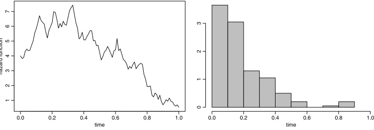
and censor the observations at a common cut-offC=0.9. The diffusion is sampled at intervals of length 0.01, using Euler–Maruyama approximation. Figure1shows the corresponding hazards (the squared diffusion) and a histogram of sampled data. The hazard function has a typical shape, first (mainly) increasing and then (mainly) decreasing.
We choose as time horizon of interestT =1. We then run the Hastings-within-Gibbs algorithm under the following specifications. The prior for (θ1, θ2)is Gaussian, as in Section3.1, with
Figure 1. Left: hazard functionx2. Right: histogram of data sampled fromFx,x2with censoring atC=0.9.
θ1=θ2=0 and the starting diffusion is a Brownian motion, starting atx0=2. The diffusion
path is updated on subintervals of length 0.2 at a time. The algorithm is run for 200 000 iterations and the first 2000 are discarded as burn-in.
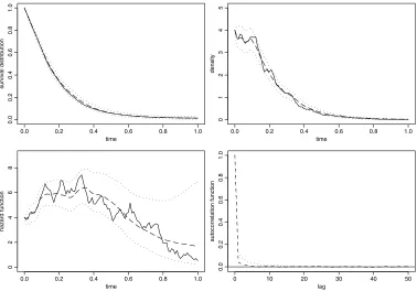
Figure2 shows the estimates of survival distribution, density and hazard function, based on the MCMC output, together with pointwise approximate 90% highest posterior bands. The true survival distribution and hazard function are also displayed to demonstrate the good fit of the MCMC estimates. Figure2also shows autocorrelation functions forθ1andθ2series.
4. Reparametrizations of the latent diffusion models
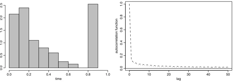
The MCMC algorithm described in the previous sections might have poor mixing properties when we consider a finite-time horizonT significantly larger than the maximum of the data. This problem is evident in Figure3. This figure shows the histogram of 200 i.i.d. observations from the distributionFx,h, wherex is a new realization of the diffusion process satisfying the
same SDE used in Section3.2; also, the hazard functionhand the censoring timeCare the same. In this simulation, we have fixed a longer time horizonT =1.8 and have then run the algorithm under the same specifications of Section3.2. Figure3displays autocorrelation functions forθ1
andθ2 series, which are not exponentially decreasing. With the same data set, but choosing a
shorter time horizon (such asT =1, as in the previous section), the algorithm does not exhibit strong serial correlation in the draws ofθ1andθ2. The worsening of the mixing properties of the
algorithm whenT becomes significantly larger than the maximum of the data was also observed for the data set simulated in Section3.2.
Figure 2. Upper-left: true survival distribution 1−Fx,x2(solid), together with its posterior mean (dashed)
and pointwise approximate 90% highest posterior bands (dotted). Upper-right: true density (solid), to-gether with its posterior mean (dashed) and pointwise approximate 90% highest posterior bands (dotted). Lower-left: true hazard functionx2(solid), together with its posterior mean (dashed) and pointwise approxi-mate 90% highest posterior bands (dotted). Lower-right: autocorrelation functions forθ1series (dotted) and
θ2series (dashed).
received much attention. See, for example,Hills and Smith(1992),Gelfand, Sahu and Carlin (1995),Gelfand, Sahu and Carlin(1996) andPapaspiliopoulos, Roberts and Sköld(2003, 2007). Instead of using the natural parametrization of the model in terms of (, X), the so-called
centered parametrization, we parametrize it in terms of(,X), where
Xt=1
t≤y[n]
Xt+1
t > y[n]
Bt−By[n]
, t≥0.
In the terminology used byPapaspiliopoulos, Roberts and Sköld(2003), this is called apartially non-centered parametrization, the fullynon-centered parametrizationbeing, in this case,(, B). The diffusionXcan then be reconstructed as a function of,Xandy1, . . . , yn, by
Xt=Xt, 0≤t≤y[n],
Figure 3. Left: histogram of data sampled fromFx,x2 with censoring atC=0.9. Right: autocorrelation
functions forθ1series (dotted) andθ2series (dashed).
The joint posterior distribution of andX has density, with respect to the product measure Ld⊗Wσ, given by
π(θ,x˜|y1, . . . , yn)=Cp(θ )g
x[0,y[n]]|θ
ly1, . . . , yn|x[0,y[n]]
, (14)
wherex[0,y[n]]≡ ˜x[0,y[n]], C is a normalizing constant and g(x[0,y[n]]|θ )=
dPy[n],θ
dWy[n],σ(x[0,y[n]])is
given by Girsanov’s formula (2). Note, in particular, that (14) characterizes the posterior dis-tribution ofX, and thus the posterior distribution of the diffusion X, over the whole positive half-line. It thus also highlights thatX[0,y[n]]acts as sufficient statistics.
It is possible to simulate from (14) by means of a Gibbs sampler quite similar to the one described in Section3.1. However, the algorithm is now completely robust to the choice ofT since the update of the parameter, conditionally onX, only involves X[0,y[n]]. In the first step,
in fact, we now simulateconditionally onX[0,y[n]]. In the second step, we simulateXover the
time interval of interest,[0, T], conditionally onand the observations. In this case, we use a proposal distribution which is a Brownian motion starting atx0over the time interval[0, y[n]]and
a Brownian motion starting at 0 over the time interval[y[n], T]. On[0, y[n]], we again follow the
updating strategy with the overlapping Brownian bridges that was described in Section3.1. When reconstructing the diffusionX[0,T]fromandX[0,T], we are careful to preserve the continuity
of the diffusion path at timey[n]. Details are omitted.
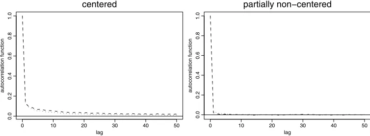
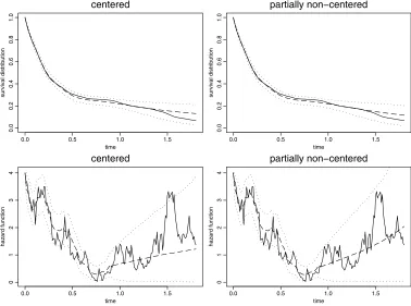
Figures4and5compare mixing and MCMC estimates obtained with the algorithms based on the centered parametrization and on the partially non-centered parametrization for the data set corresponding to Figure3. The specifications of the two algorithms are as in Section3.2. Note that the hazard function is bathtub shaped. Hazard functions with such a shape are quite common in survival analysis (think, for instance, of human mortality).
As we shall see in Section6, another reparametrization of the model, one that turns out to be useful in the presence of covariates, is the fullynon-centered parametrizationin terms of(, B). The diffusionXcan be reconstructed as a function ofandB, simply by the SDE
Figure 4. Autocorrelation functions forθ1series (dotted) andθ2series (dashed), obtained with the
algo-rithm based on the centered parametrization (left) and with the algoalgo-rithm based on the partially non-centered parametrization (right).
The joint posterior distribution of andB has density, with respect to the product measure Ld⊗Wσ, given by
π(θ, b|y1, . . . , yn)=Cp(θ )l
y1, . . . , yn|θ, b[0,y[n]]
, (15)
whereC is a normalizing constant andl(y1, . . . , yn|θ, b[0,y[n]])=l(y1, . . . , yn|x[0,y[n]])is as in (4). Note that, similarly to what has been observed for the partially non-centered parametrization, (15) also characterizes the posterior distribution of the diffusionXover the whole positive half-line. Moreover, the Gibbs sampler that simulates from (15) is also completely robust with respect to the choice of the time horizonT. In the first step, we simulateconditionally onB[0,y[n]]and
the observations. Note, in particular, that the conditional distribution of, givenB[0,T]and the
observations, now has density, with respect toLd, proportional top(θ )l(y1, . . . , yn|θ, b[0,y[n]]). In the second step, we simulate B over the time interval of interest, [0, T], conditionally on and the observations. For proposal distribution, we use a Brownian motion starting at 0 and we employ the updating strategy based on overlapping Brownian bridges. In this case, when updating the Brownian motion pathbover the subinterval[ti, ti+2], we need to reconstruct the
corresponding diffusion pathx over the subinterval[ti, T]in order to preserve the continuity of
the diffusion path at timeti+2. Details are omitted.
5. Latent diffusion models for multiple groups of observations
We now discuss a straightforward generalization of the framework developed in the previous sections and deal with the case of multiple groups of observations, where the observations within each group are taken under homogeneous conditions. Consider, for example, the case in which different treatments are being administered to different groups of patients in a clinical trial.
Figure 5. Top: true survival distribution distribution 1−Fx,x2 (solid), together with its posterior mean
(dashed) and pointwise approximate 90% highest posterior bands (dotted), obtained with the algorithm based on the centered parametrization (left) and with the algorithm based on the partially non-centered parametrization (right). Bottom: true hazard functionx2(solid), together with its posterior mean (dashed) and pointwise approximate 90% highest posterior bands (dotted), obtained with the algorithm based on the centered parametrization (left) and with the algorithm based on the partially non-centered parametrization (right).
of observations(Yn[1])n, . . . , (Yn[q])nsuch that the random variables in((Yn[1])n, . . . , (Yn[q])n)are
conditionally independent, givenFX[1],h, . . . , FX[q],h, and the random variables in(Y[ k] n )n have
common distributionFX[k],hfork=1, . . . , q.
The joint distribution ofY1[1], . . . , Yn[11], . . . , Y [q]
1 , . . . , Y
[q]
nq , givenX[
1]=x[1], . . . , X[q]=x[q],
has density, with respect toLn(wheren=n1+ · · · +nq), given by
ly1[1], . . . , yn[1] 1;. . .;y
[q]
1 , . . . , y[
q] nqx
[1]
[0,y[n1]], . . . , x [q]
[0,y[nq]]
=
q
k=1
ly[1k], . . . , y[nk]
kx
[k]
[0,y[nk]]
,
wherey[nk]:=max{y
[k]
1 , . . . , y[
k]
nk}andl(y
[k]
1 , . . . , y[
k] nk|x
[k]
[0,y[nk]])is as in (4). Using the partially
X[1], . . . ,X[q]has density, with respect to the product measureLd⊗Wqσ, given by
πθ,x˜[1], . . . ,x˜[q]y1[1], . . . , yn[1] 1;. . .;y
[q]
1 , . . . , y
[q] nq
(16)
=Cp(θ )
q
k=1
gx[[0k,y] [nk]]|θ
ly1[k], . . . , yn[k]
kx
[k]
[0,y[nk]]
,
whereCis a normalizing constant andg(x[[0k,y]
[nk]]|θ )=
dPy[nk],θ
dWy[nk],σ(x
[k]
[0,y[nk]])is given by Girsanov’s
formula (2).
The contributions of theq groups of observations factorize in (16) and a simple modification of the MCMC algorithm presented in the previous sections may be used to deal with this case. LetT1, . . . , Tqbe the time horizons of interest for theq groups, withTk≥y[nk]fork=1, . . . , q.
The Hastings-within-Gibbs algorithm for sampling from (16) alternates between 1. simulation of, conditional on the current paths ofX[[10],y
[n1]], . . . ,X
[q]
[0,y[nq]];
2. for eachkin{1, . . . , q}, simulation ofX[[k0],T
k], conditional on the observationsY
[k]
1 , . . . , Y[
k] nk
and the current value of.
Consider, for example, a latent diffusion model withq stochastically independent diffusion processes,X[1], . . . , X[q], satisfying the SDE (10). Choose the same multivariate Gaussian prior forthat was used in Section3.1. Then, the distribution of, givenX[[10,y]
[n1]]=x
[1]
[0,y[n1]], . . . ,
X[[0q,y] [nq]]=x
[q]
[0,y[nq]], is still Gaussian, with mean vector and covariance matrix as in (11), but
with
Si:=
1 σ2
q
k=1
y[nk]
0
fi
x[tk]dxt[k]
+
d
j=1
λijμj,
Lij:=
1 σ2
q
k=1
y[nk]
0
fi
x[tk]fj
xt[k]dt
+λij
fori=1, . . . , d,j=1, . . . , d. The update of the parametercan thus be performed by sampling directly from this conditional distribution. The second step may be carried out byq repetitions of the updating mechanism described in Sections3.1and4.
5.1. An illustrative application to a real data set with multiple groups of
observations
In this section, we show the implementation of the latent diffusion model for multiple groups of observations via an illustrative application to a small data set from a clinical trial, one that has been considered in a number of papers in the context of survival analysis, among themGehan (1965),Cox(1972),Wei(1984) andXu and O’Quigley(2000) in the non-Bayesian literature andKalbfleisch (1978), Laud, Damien and Smith(1998) and Damien and Walker (2002) in the Bayesian literature. In the trial, reported byFreireich(1963), 6-mercaptopurine (6-MP) was compared to a placebo in the maintenance of remission in acute leukemia. The following lengths of remission in weeks were recorded for 42 patients, half of which treated with the 6-MP drug and half with the placebo (a+sign indicates a censored observation):
6-MP: 6, 6, 6, 6+, 7, 9+, 10, 10+, 11+, 13, 16, 17+, 19+, 20+, 22, 23, 25+, 32+, 32+, 34+, 35+,
placebo: 1,1,2,2,3,4,4,5,5,8,8,8,8,11,11,12,12,15,17,22,23.
We thus consider a model for two groups of observations, namely the 6-MP drug group and the placebo group. As latent diffusion model, we shall use the stochastic perturbation around the Weibull described in Section2.1. Recall that this model has base diffusion satisfying the SDE
dXt=θ1(sign(Xt))|Xt|θ2dt+σdBt, t≥0, X0=x0>0,
and hazard functionh(u)= |u|.
We express the data as fractions of one year and choose as time horizons of interestT1=T2=
0.75, corresponding to 9 months (39 weeks). We take 1 and2to be a priori independent,
with a Gaussian prior distribution for1, meanμ=0, variance 1/λ=5, and a uniform prior
over[0,1]for2. Moreover, we setx0=0.8 andσ=8. We then run the Hastings-within-Gibbs
algorithm based on the partially non-centered parametrization. The update of1 is performed
by sampling directly from the conditional distribution1, given2,X[[10,y][n
1]],
X[[02],y
[n2]], which
is still Gaussian with meanSL++λμλ and varianceL+1λ, where
S:= 1 σ2
2
j=1
y[nj]
0
signxt[j]xt[j]θ2dxt[j]
and L:= 1 σ2
2
j=1
y[nj]
0
xt[j]θ22dt
.
For the update of2, we use an independence sampler with a Beta proposal distribution, with
parameters(1/2,1/2). The update ofX[1] andX[2] is carried out as described in the previous sections. The algorithm is run for 200 000 iterations and the first 2000 are discarded as burn-in.
Figure 6. Left: posterior mean survival distributions and pointwise approximate 90% highest posterior bands for the group of patients treated with 6-MP drug (solid) and for the group of patients treated with the placebo (dashed), together with corresponding Kaplan–Meier curves. Right: posterior mean hazards for the group of patients treated with 6-MP drug (solid) and for the group of patients treated with the placebo (dashed).
We could now verify the efficacy of 6-MP drug treatment as proposed inDamien and Walker (2002). In particular, under the hypothesis that the 6-MP drug is inefficient, we would regard all patients as belonging to a single group, instead of two. We could then implement the latent diffusion model based on the stochastic perturbation of the Weibull, but with just one diffusion process. Let M1 denote the model where all patients belong to a single group (corresponding
to the hypothesisH1of null efficacy of the 6-MP drug) and let M2denote the model
consid-ered above (corresponding to the hypothesisH2 of efficacy of the 6-MP drug). If the a priori
probabilities of hypothesesH1andH2are set equal to 0.5, the Bayes factor
BF=probability density of data under model M1 probability density of data under model M2
gives the posterior odds in favor ofH1. As expected, the computed Bayes factor (BF=9×10⁻⁶)
provides strong evidence for the efficacy of the 6-MP drug.
6. Latent diffusion models with covariates
Covariates can be included in the latent diffusion models described in a very natural way, as di-rectly influencing the underlying diffusion. For instance, ifZis a vector ofpcovariates measured at time 0, we can use the model based on the diffusion satisfying the SDE
dXt=β(Xt,z, θ )dt+σdBt, t≥0,
(17) X0=x0(z, θ ).
underlying process that leads to the event has advanced (such as staging measures in cancer) may be taken to influence the starting point of the diffusion. Those covariates which instead represent causal influence on the development of the process may be taken to influence the drift of the diffusion.
Letztake valuesz[1], . . . ,z[q]. Then, (17) givesqdifferent diffusions,X[z=z[1]], . . . , X[z=z[q]], driven by the same Brownian motionB, with
dXt[z=z[k]]=β
X[tz=z[k]],z[k], θdt+σdBt, t≥0,
X0=x0
z[k]
fork=1, . . . , q. Denote byF
X[z=z[1]]
,h, . . . , FX[z=z[q]]
,h the relative random distributions, as in
(3). Moreover, denote by Y1[z=z[k]], . . . , Yn[zk=z[k]] the survival times of the nk individuals
hav-ing covariatesz=z[k] for k=1, . . . , q. The survival timesY1[z=z[k]], . . . , Yn[zk=z[k]],
condition-ally onF
X[z=z[k]],h, are i.i.d. with common distributionFX[z=z[k]],h. Since theq diffusions are
driven by the same Brownian motion, it is here more natural to use the fully non-centered parametrization of the model, described in Section 4. In particular, the joint distribution of Y1[z=z[1]], . . . , Yn[z1=z[1]], . . . , Y
[z=z[q]]
1 , . . . , Y[
z=z[q]]
nq ,givenB=band=θ, has density, with
re-spect toLn(wheren=n1+ · · · +nq), given by
ly1[z=z[1]], . . . , yn[z=z[1]] 1 ;. . .;y
[z=z[q]]
1 , . . . , y[
z=z[q]]
nq θ, b[0,y[n]],z[
1], . . . ,z[q]
=
q
k=1
ly1[z=z[k]], . . . , yn[z=z[k]]
k θ, b[0,y[nk]],z[
k],
wherey[n]:=max{y1, . . . , yn},y[nk]:=max{y
[z=z[k]]
1 , . . . , y[
z=z[k]]
nk }and
ly1[z=z[k]], . . . , yn[z=z[k]]
k θ, b[0,y[nk]],z[
k]=ly[z=z[k]]
1 , . . . , y[
z=z[k]]
nk x
[z=z[k]]
[0,y[nk]]
is as in (4). The joint posterior distribution ofandB has density, with respect to the product measureLd⊗Wσ, given by
πθ, by1[z=z[1]], . . . , yn[z=z[1]] 1 ;. . .;y
[z=z[q]]
1 , . . . , y[
z=z[q]]
nq ;z
[1], . . . ,
z[q]
(18)
=Cp(θ ) q
k=1
ly1[z=z[k]], . . . , yn[z=z[k]]
k θ, b[0,y[nk]],z[
k].
Note that this model is structurally different from the model for multiple groups of observa-tions described in Section5 since the distributions of the survival times are here linked at the level of the Brownian motion, allowing a much stronger borrowing of strength for inference across individuals who share a common value of even just one of thepcovariates.
As usual, we denote byT the time horizon of interest,T ≥y[n]. The Hastings-within-Gibbs
1. simulation of, conditional on the current path ofB[0,y[n]], the observations and the
co-variates;
2. simulation ofB[0,T], conditional on the current value of, the observations and the
covari-ates.
In particular, the update of the Brownian motionB[0,T]can be carried out via the updating
strat-egy based on overlapping Brownian bridges, as described in Section4.
6.1. An illustrative application to a real-world data set with covariates
In this section, we illustrate how to efficiently handle the model with covariates via an application to a data set concerning 272 patients diagnosed with non-small cell lung cancer. The data set is described in detail inMuers, Shevlin and Brown(1996). Survival times are measured in months from the time of diagnosis (with 17% of censoring) and some covariates are recorded at the time of diagnosis. Just to give an illustration of the model, we shall consider here two covariates: sex (F =0: male andF =1: female) and hoarseness (H=0: absent andH=1: present). Using, for instance, the model based on the stochastic perturbation around the Weibull, we can include these covariates as follows:
dXt=exp{θ10+θ11F}(sign(Xt))|Xt|θ2dt+σdBt, t≥0,
X0=exp{θ00+θ01F +θ02H}.
Note that, following the suggestion of Aalen, Borgan and Gjessing(2008), we have modeled the covariate hoarseness, which only represents a measure of how far the lung tumor has ad-vanced, as influencing the starting point of the diffusion; we have instead taken the covariate sex to influence both the starting point and the drift of the diffusion, in order to account for possi-ble differences between males and females, both in the hazards at time of diagnosis and in the hazard dynamics. The covariate combinations determine four different diffusions,X[F=0,H=0], X[F=0,H=1],X[F=1,H=0]andX[F=1,H=1], driven by the same Brownian motion. According to
this model, the hazard at time 0 (the time of diagnosis) of patients suffering from hoarseness is exp{θ02}times that of patients not suffering from hoarseness and the hazard at time 0 of
fe-male patients is exp{θ01}times that of male patients; moreover, exp{θ11}gives a measure of the
different progression rate of the cancer in female patients with respect to male patients.
We express the data as fractions of a quadrennium and choose as time horizonT the maximum of the observations, corresponding to about 37 months. In order to avoid dependencies among the (θ00, θ01, θ02)parameters and among the(θ10, θ11)parameters, we reparametrize them in terms
of(η00, θ01, θ02)and(η10, θ11), withθ00=η00−pFθ01−pHθ02andθ10=η10−pFθ11, where
we have denoted bypF andpH the percentage of females patients and the percentage of patients
suffering from hoarseness, respectively. We take all of the parameters to be a priori independent, with Gaussian priors with mean 0 and variance 5 for all parameters except2, for which we
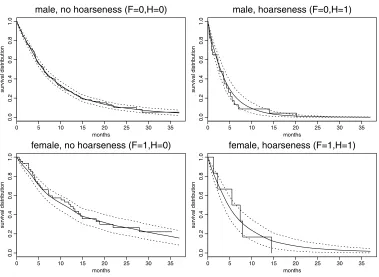
Figure 7. Left: posterior mean survival distributions, together with Kaplan–Meier curves, for male pa-tients without hoarseness at time of diagnosis (F=0, H=0, solid line), for male patients with hoarseness (F=0, H=1, dotted and dashed line), for female patients without hoarseness (F=1, H=0, dashed line) and for female patients with hoarseness (F=1, H=1, dotted line). Right: the same for posterior mean hazard functions.
Figure 7 shows posterior mean survival distributions, together with Kaplan–Meier curves, for male patients without hoarseness at time of diagnosis (F =0, H =0, solid line), for male patients with hoarseness (F =0, H =1, dotted and dashed line), for female patients without hoarseness (F =1, H=0, dashed line) and for female patients with hoarseness (F =1, H=1, dotted line). The four survivals are also plotted separately in Figure8with 90% highest posterior bands. Figure7also displays the posterior mean hazard functions for the four covariate combi-nations. In particular, the posterior mean hazard at time 0 of patients suffering from hoarseness is 2.2 times bigger than that of patients not suffering from hoarseness, whereas the hazard at time 0 of female patients is 0.6 times that of male patients.
Note that even though we have only considered categorical covariates in this illustrative appli-cation, quantitative covariates can also be included in the model; however, it may be necessary to categorize these covariates in order to have a sufficient number of observations for each of the diffusion processes. This, of course, requires larger data sets.
7. Generalization to the case of unknown diffusion coefficient
An important generalization of the models we have considered thus far consists of considering diffusion processes with unknown diffusion coefficientσ sinceσ describes a natural measure of prior uncertainty. We briefly discuss how to deal with this case.
Letbe a real random variable. Given=θand=σ, consider the scalar diffusion process Xsolution of the SDE (1) and denote byPT ,θ,σ the law ofX[0,T]. Letp(·)be the prior density,
with respect toL, of(for simplicity, we takeandto be stochastically independent a pri-ori). Let us consider, for instance, the centered parametrization of the model. The joint posterior distribution of(, , X[0,T])has density, with respect toLd+1⊗WT ,σ, given by
πθ, σ, x[0,T]|y1, . . . , yn
=Cp(θ )p(σ )g
x[0,T]|θ, σ
ly1, . . . , yn|x[0,y[n]]
Figure 8. Upper-left: posterior mean survival distribution and pointwise approximate 90% highest poste-rior bands, together with Kaplan–Meier curve, for male patients without hoarseness. Upper-right: the same for male patients with hoarseness. Lower-left: the same for female patients without hoarseness. Lower-right: the same for female patients with hoarseness.
whereC is a normalizing constant andg(x[0,T]|θ, σ ):=
dPT ,θ,σ
dWT ,σ (x[0,T])is given by Girsanov’s
formula (2).
The quadratic variation of a diffusion processes, having diffusion coefficientσ, satisfies
lim
m→∞
m
i=1
Xt i/m−Xt (i−1)/m 2
=t σ2, WT ,σ-a.s. for allt.
Therefore, the conditional distribution of, given the diffusionX[0,T], degenerates to a point
mass and is completely determined by the diffusion path. In practice, we cannot simulate the diffusion path in continuous time, but just at discrete time instants. In any case, the finer the discrete-time approximation{XiT /m: i=1, . . . , m}of the diffusionX[0,T], the stronger the
dependence between{XiT /m: i=1, . . . , m}and. Consider the algorithm for the simulation
from (19) that alternates between:
1. simulation of, conditional on the current value ofand the current path ofX[0,T];
3. simulation ofX[0,T], conditional on the observations and the current values ofand.
The finer the approximation of the diffusion path, the worse the convergence of the algorithm becomes. In the limiting casem= ∞(i.e., if the diffusion process could be simulated in con-tinuous time), this scheme would be reducible; seeRoberts and Stramer(2001). An alternative way to see this problem is to note that the collection of measures{WT ,σ: σ ∈R}are mutually singular and, therefore, so are the measures{PT ,θ,σ: σ∈R}.
In this case, the need for a different parametrization of the model is thus compelling. Following Roberts and Stramer(2001), we parametrize the model in terms of(, ,X), where˙ X˙t=(Xt−
X0)/. By Itô’s formula,
dX˙t=
β(X˙t, )
dt+dBt, t≥0, X˙0=0.
The distribution ofX˙[0,T] depends on, but any realization ofX˙[0,T] contains only finite
in-formation about. Analogous reparametrizations are derived starting from the ones described in Section4. MCMC algorithms based on these reparametrizations can be obtained as simple modifications of the ones previously described.
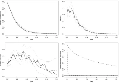
Consider the toy example described in Section3.2and assume the same model, but let the diffusion process have an unknown diffusion coefficient. Let the prior for this coefficient be exponential with mean 1. Figure9displays the results obtained with the MCMC algorithm based on the reparametrization(, ,X). Specifications of the algorithm are as in Section˙ 3.2. Note that the mixing forσ is slow relative to the very good mixing forθ1 andθ2, but this does not
prevent good estimates of the survival distribution, density and hazard being obtained. Slow mixing forσ could probably be improved by a further reparametrization of the model.
Alternatively to the case of an unknown diffusion coefficient, it would be possible to consider models based on diffusion processes havingσ =1, but with hazard functionh(, X), where is a random parameter. A reparametrization of the model would also be necessary in this case.
8. Discussion
In this paper, we have described latent diffusion models for survival analysis and have shown that these models can be efficiently treated by means of MCMC techniques. We have dealt with the case of multiple groups of observations, typical of clinical trials, and we have shown how covari-ates can be efficiently included in the models. We have outlined how, in the described framework, it is possible to consider stochastic perturbations of common survival models. In particular, we have used a stochastic perturbation of the Weibull model in some illustrative applications to small data sets, with multiple groups of observations and with covariates. Applications to larger data sets, where the potential of a latent diffusion model may be fully expressed, will be the object of future work. All analyses presented are computationally feasible within R (seeR Development Core Team(2007)).
associ-Figure 9. This corresponds to Figure 2, but for the model with unknown diffusion coefficient. The lower-right plot also displays the autocorrelation function forσ series (dotted-dashed line).
ated with random probabilities based on diffusions are smooth, being the integrals of continuous processes. By replacing the diffusion process with a jump diffusion process, it would be possi-ble to capture sudden changes in the behavior of cumulative hazards that might be due to some kind of shock experienced by the population. Hazards modeled through stochastic processes with jumps have been studied, for instance, byGjessing, Aalen and Hjort(2003).
Acknowledgments
[image:23.488.69.448.54.319.2]References
Aalen, O.O., Borgan, Ø. and Gjessing, H.K. (2008).Survival and Event History Analysis. A Process Point of View. New York: Springer.MR2449233
Aalen, O.O. and Gjessing, H.K. (2001). Understanding the shape of the hazard rate: A process point of view (with discussion).Statist. Sci.161–22.MR1838599
Aalen, O.O. and Gjessing, H.K. (2004). Survival models based on the Ornstein–Uhlenbeck process.Lifetime Data Anal.10407–423.MR2125423
Beskos, A., Papaspiliopoulos, O., Roberts, G.O. and Fearnhead, P. (2006). Exact and computationally effi-cient likelihood-based estimation for discretely observed diffusion processes.J. R. Stat. Soc. Ser. B Stat. Methodol.68333–382.MR2278331
Cox, D.R. (1972). Regression models and life-tables (with discussion).J. R. Stat. Soc. Ser. B Stat. Methodol. 34187–220.MR0341758
Damien, P. and Walker, S. (2002). A Bayesian non-parametric comparison of two treatments.Scand. J. Statist.2951–56.MR1894380
Doksum, K. (1974). Tailfree and neutral random probabilities and their posterior distributions.Ann. Probab. 2183–201.MR0373081
Dykstra, R.L. and Laud, P. (1981). A Bayesian nonparametric approach to reliability.Ann. Statist.9356– 367.MR0606619
Elerian, O., Chib, S. and Shephard, N. (2001). Likelihood inference for discretely observed nonlinear dif-fusions.Econometrica69959–993.MR1839375
Ferguson, T.S. (1974). Prior distributions on spaces of probability measures.Ann. Statist. 2615–629.
MR0438568
Ferguson, T.S. and Phadia, E.G. (1979). Bayesian nonparametric estimation based on censored data.Ann. Statist.7163–186.MR0515691
Freireich, E.O. (1963). The effect of 6 mercaptopurine on the duration of steroid induced remission in acute leukemia.Blood21699–716.
Gehan, E.A. (1965). A generalized Wilcoxon test for comparing arbitrarily singly-censored samples. Bio-metrika52203–223.MR0207130
Gelfand, A.E., Sahu, S.K. and Carlin, B.P. (1995). Efficient parameterisations for normal linear mixed models.Biometrika82479–488.MR1366275
Gelfand, A.E., Sahu, S.K. and Carlin, B.P. (1996). Efficient parametrizations for generalized linear mixed models. InBayesian Statistics5165–180. New York: Oxford Univ. Press.MR1425405
Gjessing, H.K., Aalen, O.O. and Hjort, N.L. (2003). Frailty models based on Lévy processes.Adv. in Appl. Probab.35532–550.MR1970486
Hills, S.E. and Smith, A.F.M. (1992). Parameterization issues in Bayesian inference. InBayesian Statistics 4227–246. New York: Oxford Univ. Press.MR1380279
Hjort, N.L. (1990). Nonparametric Bayes estimators based on beta processes in models for life history data.
Ann. Statist.181259–1294.MR1062708
Ishwaran, H. and James, L.F. (2004). Computational methods for multiplicative intensity models using weighted gamma processes: Proportional hazards, marked point processes and panel count data.J. Amer. Statist. Assoc.99175–190.MR2054297
Kalbfleisch, J.D. (1978). Non-parametric Bayesian analysis of survival time data.J. R. Stat. Soc. Ser. B Stat. Methodol.40214–221.MR0517442
Kloeden, P.E. and Platen, E. (1992). Numerical solution of stochastic differential equations. InApplications of Mathematics23. Berlin: Springer-Verlag.MR1214374
Lo, A.Y. and Weng, C.-S. (1989). On a class of Bayesian nonparametric estimates. II. Hazard rate estimates.
Ann. Inst. Statist. Math.41227–245.MR1006487
Muers, M.F., Shevlin, P. and Brown, J. (1996). Prognosis in lung cancer: Physicians’s opinions compared with outcome and a predictive model.Thorax51894–902.
Myers, L.E. (1981). Survival functions induced by stochastic covariate processes.J. Appl. Probab.18523– 529.MR0611796
Papaspiliopoulos, O., Roberts, G.O. and Sköld, M. (2003). Non-centered parameterizations for hierarchical models and data augmentation (with discussion). InBayesian Statistics7307–326. New York: Oxford Univ. Press.MR2003180
Papaspiliopoulos, O., Roberts, G.O. and Sköld, M. (2007). A general framework for the parametrization of Hierarchical models.Statist. Sci.2259–73.MR2408661
R Development Core Team (2007).R: A Language and Environment for Statistical Computing. Vienna, Austria: R Foundation for Statistical Computing. ISBN 3-900051-07-0.
Roberts, G.O. and Stramer, O. (2001). On inference for partially observed nonlinear diffusion models using the Metropolis–Hastings algorithm.Biometrika88603–621.MR1859397
Rogers, L.C.G. and Williams, D. (2000).Diffusions, Markov Processes, and Martingales, Volume 2: Itô Calculus.Cambridge Mathematical Library, Cambridge: Cambridge Univ. Press.
Shephard, N. and Pitt, M.K. (1997). Likelihood analysis of non-Gaussian measurement time series. Bio-metrika84653–667.MR1603940
Stroock, D.W. and Varadhan, S.R.S. (2006).Multidimensional Diffusion Processes. Berlin: Springer-Verlag.
MR2190038
Susarla, V. and Van Ryzin, J. (1976). Nonparametric Bayesian estimation of survival curves from incom-plete observations.J. Amer. Statist. Assoc.71897–902.MR0436445
Wei, L.J. (1984). Testing goodness of fit for proportional hazards model with censored observations.
J. Amer. Statist. Assoc.79649–652.MR0763583
Woodbury, M.A. and Manton, K.G. (1977). A random-walk model of human mortality and aging.Theoret. Population Biology1137–48.MR0490068
Xu, R. and O’Quigley, J. (2000). Proportional hazards estimate of the conditional survival function.J. R. Stat. Soc. Ser. B Stat. Methodol.62667–680.MR1796284
Yashin, A.I. (1985). Dynamics of survival analysis: Conditional Gaussian property versus the Cameron– Martin formula. InStatistics and Control of Stochastic Processes466–485. New York: Optimization Software.MR0808217
Yashin, A.I. and Vaupel, J.W. (1986). Measurement and estimation in heterogeneous populations. In Im-munology and Epidemiology.Lecture Notes in Biomath.65198–206. Berlin: Springer.MR0849172