The Perdigão field campaign : evaluation of the Cell Perturbation Method in atmospheric simulations

1

Faculty of Electrical Engineering,

Mathematics & Computer Science

The Perdig˜ao Field Campaign:

Evaluation of the

Cell Perturbation Method

in Atmospheric Simulations

Leendert van Veen

April 11, 2018

Graduation committee:

Chairman: Prof. dr. ir. B.J. Geurts

Multiscale Modeling and Simulation Applied Mathematics University of Twente

Supervisor: Prof dr. ir. F.K. Chow

Environmental Fluid Mechanics and Hydrology Civil and Environmental Engineering University of California, Berkeley

Independent member: Dr. H.G.E Meijer

Abstract

State-of-the-art modeling methods are used to simulate the flow over highly complex terrain

as documented during the 2017 Perdig˜ao Field Campaign (Portugal). A one-way nesting

tech-nique in the Weather Research and Forecasting (WRF) model distinguishing four levels is used

to capture the broad range of scales of motion. A new coupling strategy, the Cell

Perturba-tion Method (CPM), is adopted and evaluated using the field data of the campaign. To what

extent CPM is contributing to the numerical predictions is the main question addressed in this

research. Different model configurations are compared and both qualitative and quantitative

comparisons are evaluated to demonstrate the contributions of CPM to the overall results. The

domain definition is found important and the robustness of CPM is shown by field comparisons.

Wind direction comparisons with tower data of eight different towers show a better agreement

for towers measuring the mean flow. Wind speed is under-predicted for all the towers and only

the average magnitude of the prediction of turbulent kinetic energy (TKE) has a reasonable

agreement with some of the tower data. Comparison with a simulations without CPM shows

Contents

1 Introduction 5

2 Dataset: Perdig˜ao Field Campaign 8

2.1 General Background . . . 8

2.2 Measurement Equipment . . . 10

3 Numerical Setup 11

3.1 WRF Numerical Scheme . . . 11

3.2 Multiscale Modeling Strategy . . . 13

3.3 Cell Perturbation Method . . . 16

4 Assessment of Simulation Results using Perdig˜ao Field Data 20

4.1 Robustness of the Cell Perturbation Method . . . 20

4.2 Domain Configuration . . . 22

4.3 Comparison to Field Data . . . 25

1

Introduction

Mesoscale to microscale modeling can be used to efficiently represent the broad range of scales

of motion in atmospheric flows. Mesoscale modeling is typically done with resolutions of

O(1− 10km) , while microscale modeling uses a much finer resolution, O(1− 10m). At the largest mesoscale grids, turbulence is only represented in an average sense, while at finer

scales the resolution is fine enough to resolve some of the energy-containing eddies. Using

grid nesting, the comparably smooth solution from the mesoscale grid can be interpolated to a

nested, much finer grid to represent lateral boundary conditions for the Large Eddy Simulation

(LES). As a consequence, the lateral boundary conditions imposed on the nested LES domain

do not contain the energy scales required to match the three-dimensional eddies which can be

resolved on the LES domain.

Recent work has developed a technique to computationally ‘enhance’ the mesoscale

solu-tion imposed at the LES boundaries which needs to improve the coupling between the nested

models. Small scale energy is introduced with the aim of significantly speeding up the

numer-ical transition from the rather smooth solution imposed at the boundaries of the LES domains.

These leads to a much more energetic representation of the finer scales which are resolvable in

the nested LES domain. This has the virtue of reducing computational costs, since nested LES

domain does not have to be enlarged to represent the same energetic representation of the finer

scales. In this research we exploit the recent 2017 Perdig˜ao Field Campaign data to support

a first validation of the so-called cell perturbation method (CPM), as pioneered by

Mu˜noz-Esparza et al. [2014], when applied to flow over highly complex terrain. To what extent CPM

contributes to the quality of numerical predictions is the main question addressed in this report.

Generating the appropriate turbulent length scales at inflow boundaries has been a

ap-plications ranging from hybrid RANS-LES models in aerodynamics modeling [Lardeau et al.,

2007] to multiple level nested modeling in atmospheric boundary layer modeling [Mirocha

et al., 2014]. A well known method is the so-called recycling method [Lund et al., 1998]. This

method computes the solution of the flow at a vertical plane located in the LES domain

paral-lel to the inflow boundary and uses this solution as lateral boundary condition for the domain

of interest at each time step. This way the flow at the inlet of the domain is fully developed.

However, due to the recycling technique of the flow solution, periodicity may influence the

flow solution. In case of a nested atmospheric flow model with variable inflow and outflow

conditions along each boundary, measurement data can be used to generate consistent

bound-ary conditions. Nakayama et al. [2012] used a recycling strategy to generate turbulence for

a boundary-layer flow over urban areas. The fluctuating components at a downstream station

were added to the mean winds at the inflow. This method showed promising results. However,

the method is hard to implement when the dominant wind-direction changes in time.

As an easy-to-implement method, Mirocha et al. [2014] examined the addition of sinusoidal

perturbations in both horizontal directions to the potential temperature and velocity fields on the

nested LES domain near the inflow boundaries. The added perturbations accelerated the

forma-tion of turbulent structures in simulaforma-tions of neutral atmospheric condiforma-tions. In this method it

is a challenge to define the different parameters of the perturbations, e.g., magnitude, timescale

and location of the perturbations. Mu˜noz-Esparza et al. [2014] tested different methods based

on direct perturbation of the potential temperature field. They found their cell perturbation

method (CPM) to be the simplest and most efficient in accelerating the generation of

small-scale dynamic content in the numerical turbulence. This method superimposes pseudo-random

perturbations to the solution at grid points near the inflow boundary. In fact, the same

forcings. Important parameters were identified and suitable values were advised for various

atmospheric conditions.

CPM was initially developed for numerically accelerating the transition between a smooth

mesoscale solution and a full three-dimensional turbulent flow. Recently, different papers have

highlighted the advantage of using such a perturbation method also when the solution from the

parent domain contains (under-resolved) turbulence. Mirocha et al. [2014] found that adding

perturbations on lateral boundaries of a fine LES domain nested within a coarse LES domain

significantly accelerated the development of turbulence. In this approach, small scales were

added to inertial range eddies advecting in from the parent domain. Mazzaro et al. [2017]

showed that the cell perturbation method can be beneficial when the solution on the parent

mesoscale domain contains under-resolved convection. The under-resolved convective

struc-tures may be broken down to smaller strucstruc-tures by the perturbation method, thereby explicitly

adding to the dynamic content of the solution. Propagating such numerically added small-scale

structures with a Navier-Stokes solver may rapidly yield good approximations of the actual

turbulent flow even quite close, downstream of the perturbed cells.

These previous studies were performed for idealized setups [Mu˜noz-Esparza et al., 2015]

and over relatively flat domain [Mu˜noz-Esparza et al., 2017, J¨ahn et al., 2016]. Mu˜noz-Esparza

et al. [2017] used CPM to successfully reduce the computational cost of a diurnal cycle

simula-tion. It was found that the so-called fetch, i.e., the distance from the domain boundary needed

to develop appropriate turbulence length scales, could be significantly reduced in the

highest-resolution LES domain when perturbations were applied. CPM was applied to the LES domain,

nested within a parent mesoscale domain. For stably-stratified conditions, this approach was

also successfully applied to a second LES domain nested within a coarser LES domain.

With-out the CPM, neither of the LES domains developed turbulence, pointing at a baseline

qualitative improvements of the numerical solution, toward a genuinely turbulent flow.

The question whether CPM is beneficial in simulations over a real domain with complex

topography has not yet been addressed in literature. The generation of small-scale turbulence

on the nested domain is accelerated by the presence of finer length scales linked to the specific

topography in the domain. On the other hand, this may not be sufficient for the appropriate

turbulent length scales to develop in the domain with a reasonable fetch. In this research we

implement CPM in WRF in which we closely follow the setup of Mu˜noz-Esparza et al. [2015].

To quantify the performance of CPM, the simulated results will be compared to field data from

the Perdig˜ao campaign. This site consists of two (almost) parallel ridges surrounded by rolling

hills. Moreover, the field site has been equipped with various measurement equipment which

resulted in an unprecedented amount of available data, ready to exploit in a detailed validation.

The organization of this report is as follows. A description of the Perdig˜ao dataset which we

used to validate the computational model is given in Section 2. The numerical setup including

CPM settings that are used for these simulations can be found in Section 3. The results of

simulations and how these compare to field data can be found in Section 4. Finally, the main

findings and conclusions are summarized in Section 5.

2

Dataset: Perdig˜ao Field Campaign

2.1

General Background

The Perdig˜ao Field Campaign was part of the New European Wind Atlas (NEWA) project,

a mega-project funded by the European Union. As part of this project, the Perdig˜ao Field

Campaign focused on collecting data of mean flow and turbulent wind fields over a complex

terrain site with two parallel ridges and a single wind turbine on top of the southwest ridge. The

main focus was on better understanding the dynamics of the flow induced by complex terrain

The Perdig˜ao site is shown in Figure 2.

One of the goals of the Perdig˜ao study is to improve representation of turbulence for LES

of flow over complex terrain. Previous studies of flow over Askervein Hill [Chow and Street,

2009] showed that significant numerical errors arise due to the choice of turbulence closure

and land-surface representation. The Perdig˜ao site includes steeper and more complex terrain

compared to the Askervein Hill case which has been used as a recent benchmark for modeling

flow over complex terrain.

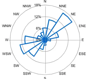
Figure 1: Wind rose for the Perdig˜ao site for a whole year. Wind is often perpendicular to the ridges.

The Perdig˜ao site features a valley, Vale do Cobr˜ao,

located near the village of Perdig˜ao. The valley is

en-closed by two (almost) parallel ridges with a length of

4 km and about 1.4 km apart. The wind direction is

often perpendicular to these ridges (Fig. 1), from both

sides, which makes the site very interesting for detailed

cross-valley flow studies. Using the dense

instrumen-tation of the site, better insight into the magnitude of

numerical errors may be achieved.

The evening transition between day and night of May 9, observed between1900−1930local time (LT), or1800−1830UCT, is selected to study the use of CPM within the Perdig˜ao case study. This date showed fairly strong south-easterly winds nearly perpendicular to the ridges

and additionally the weakly convective conditions are well-suited for studying the influence

of CPM. The height up to which the perturbations are applied is dependent on the height of

the planetary boundary layer (PBL), which increases for convective conditions and decreases

for stable, nighttime condition. Moreover, the generated perturbations are suppressed in stably

2.2

Measurement Equipment

The field site was deployed with state-of-the-art instrumentation to capture high resolution flow

characteristics. A total of 48 towers, varying in range from 10 to 100 m, were located in and

around the valley. The locations of these towers can be found in Figure 2.

Figure 2: Location of the towers at the Perdig˜ao field site with the towers labeled into four different groups. The red, star icons indicate the locations of the towers used in this research. Screenshot from Google Earth.

The layout of the towers was chosen to characterize the major features of the flow. As

shown in Figure 2, two groups of towers were located on top of the ridges, labeled ’rne’ and

’rsw’ for the NE ridgeline and SW ridgeline, respectively. A third and fourth group of towers

were located on two different transects of the valley, labeled ’tnw’ and ’tse’ for the transect at

in the valley, aligned with the ridgelines, labeled ’v’. Unfortunately, not all the measurement

equipment successfully measured the needed variables. Therefor eight different towers were

chosen for the analysis, namelyrsw06,rne06,tse13,tnw01,tnw07,v06,tse06andtse07. These

towers represented the top of both the ridgelines (rsw06, rne06 and tse13), the valley (v06,

tnw07,tse06andtse07) and the upstream conditions (tnw01). The measurements for all towers

were at 20 m above ground level (AGL), except fortse13at 100 m AGL andtse06at 60 m AGL.

By choosing these tower locations a comparison at fixed height AGL between ridges, upstream

location and the valley is possible. Moreover, the measurements at the tower locations oftse13

at the NE ridgeline andtse06in the valley can be used to compare the results higher aloft.

The towers were equipped with three dimensional sonic anemometers from which the three

dimensional wind speedsui, as well as the Reynolds stressesu0iu0j were obtained. The available

tower data had a five minute time interval. The turbulent kinetic energy (TKE) of the flow can

be computed using the Reynolds stresses, as will be explained in Subsection 4.3.

3

Numerical Setup

3.1

WRF Numerical Scheme

Multiscale simulations of the evening transition of May 9 were performed using the Weather

Research and Forecasting (WRF) model, version 3.9.1.1 [Skamarock and Klemp, 2008]. WRF

is equipped with a third-order Runge-Kutta time integration scheme and an Arakawa C-grid

staggering for spatial discretization (see figure 3).

The vertical coordinateηis terrain-following and is given by (1),

η= ph−pht

phs−pht

. (1)

with phs defined as the hydrostatic pressure at the surface of the Earth, pht the hydrostatic

Figure 3: Arakawa grid staggering with potential temperature θ, three dimensional velocity componentsu, vandwand spatial coordinatesx, yandη(from Skamarock and Klemp [2008]).

η. Eachη-level has equal hydrostatic pressure, where η = 0equals the top of the domain and η = 1describes the Earth’s surface of the domain (see Figure 4). The simulations here define the domain top aspht= 100hPa, which coincides with an altitude of approximately 15 km.

Figure 4: Vertical discretization by terrain followingη-levels (from WRF User Guide).

Aligning theη-levels with the terrain simplifies the

application of the lower boundary conditions.

How-ever, the terrain-following coordinates can cause errors

in simulations over complex terrain due to the high

as-pect ratio of the computational cells, especially when

the vertical grid spacing is decreased near the ground

[Daniels et al., 2016]. An increase in the vertical

reso-lution requires a corresponding increase of the

horizon-tal resolution to keep the aspect ratios and skewness of

the grid cells near the boundary within reasonable

lim-its. This clearly has its repercussions for the temporal

well to adhere to a CFL condition and hence maintain stability of the explicit time-stepping

method. Avoiding large aspect ratios and skewness of the grid cells when increasing the

ver-tical resolution is the main reason that simulations over complex terrain need to employ very

small time steps. This makes simulations over complex terrain particularly expensive compared

to those over flat terrain.

3.2

Multiscale Modeling Strategy

To efficiently represent the broad range of motions, a 4-domain nested setup is used, identifying

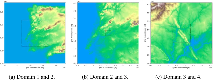
D04 ⊂ D03 ⊂ D02 ⊂ D01. The simulation thus includes motions from synoptic scales of the order of 1000 km, all the way down to turbulent eddies in the lowest part of the atmosphere

where resolutions as fine as a few meters may be achieved. The four domains are shown in

figure 5 and the sizes of the domains are given in Table 1.

(a) Domain 1 and 2. (b) Domain 2 and 3. (c) Domain 3 and 4.

Figure 5: Four domain nesting setup. Squares indicated by the dashed lines show the spatial extent of the next nested domain.

The different domains in the nested approach utilize different turbulence closure schemes.

Domains with a rather coarse resolution (∆x ≥1000m) are equipped with a mesoscale turbu-lence closure. Since the resolution of these grids is too coarse to actually resolve any turbulent

domains D01 and D02 are equipped with the Mellor-Yamada Nakanishi and Niino (MYNN)

Level 2.5 turbulence closure scheme [Nakanishi and Niino, 2004]. The choice of the MYNN

model was made following the sensitivity analysis carried out by Mu˜noz-Esparza et al. [2017].

Under convective conditions, the dominant turbulence scales are of the order of 100 m so these

can be partially resolved in D03 and D04 and subfilter-scale turbulence can be represented with

an LES closure model. In this study we employ the 1.5-order TKE closure scheme [Lilly, 1967].

All computational dimensions are listed in Table 1.

Table 1: Physical and computational dimensions of the nested grids, with nx, ny and nz the number of grid points in each dimension,∆xand∆ythe horizontal grid resolutions,∆zminthe vertical grid spacing of the first grid point, Lx (km) and Ly (km) the horizontal domain sizes and∆tthe temporal resolution.

nx ny nz ∆x(m) ∆y(m) ∆zmin(m) Lx(km) Ly (km) ∆t(s)

D01 141 141 59 6750 6750 60 945 945 30

D02 181 181 59 2250 2250 60 405 405 10

D03 241 241 71 150 150 30 27 27 0.5

D04 361 361 117 30 30 15 10.8 10.8 0.05

The resolutions of the grids on the two outermost domains D01 and D02 are∆x= 6.75,2.25

km, respectively and the resolutions of the grids on the two innermost domains D03 and D04

are∆x = 150, 30m. All the grids are uniform in x andy direction in the horizontal plane. On these grids it is possible to capture the large-scale dynamics including that induced by the

ocean on D01 and D02, as well as some of the turbulent eddies on D03 and D04. In addition, the

domain D04 was made big enough to capture the entire valley, including the ridges. The choice

of domain size of D03 is explained in Subsection 4.2. The simulations were forced in D01 by

analysis data from 0.25 by 0.25 degree global latitude and longitude grid from the Global

Fore-casting System (GFS), which is about 27.8 km by 21.4 km in the specific case of the Perdig˜ao

field site. GFS is a global weather prediction model which is initialized four times a day by the

analysis (which incorporate observation data) and predicted fields. GFS data from each interval

is interpolated to provide lower and lateral boundaries for D01 as well as initial conditions for

the simulations. The two outermost mesoscale domains, D01 and D02, are initialized on May

9, 0600 LT, D03 is initialized at 1200 LT, and D04 is initialized at 1500 LT. All the domains are

run until 1930 LT. The analysis focuses on the prediction of flow characteristics between 1900

LT and 1930 LT (1800−1830UTC), when the influence of CPM is most noticeable.

The nesting ratio between the domains D02 and D03 (∆xD02/∆xD03 = 11) is bigger than

the commonly used value of 3 to 5. The reason for this large nesting ratio is because both

mesoscale and LES closure schemes have difficulty when the resolution of the domain is in

the so-called Terra Incognita (TI) regime [Wyngaard, 2004, Zhou and Chow, 2014, Zhou et al.,

2014]. Resolutions in this regime are close to the scale of thermal plumes in the boundary

layer which extend to the boundary layer height of order O(103 _{m). Some of the convective}

cells or rolls will be resolved atO(103 _{m) resolution, rather than requiring parameterization}

through the turbulence model. This is in contrast to the assumption in mesoscale models that

the turbulence scheme captures all the turbulence and that no turbulent motions are resolved.

On the other hand, LES models running with TI resolutions also fail to accurately represent the

flow because the resolution is not fine enough to resolve all the energetic eddies. Simulation

results at TI resolutions can affect finer nested simulations by passing in erroneous information

about resolved structures [Zhou and Chow, 2014]. By adopting a large nesting ratio of 11 we

largely ’skip’ the TI regime and attempt to by-pass these complications. We do, however, put

significant emphasis on the generation of appropriate scales using this nesting strategy, which

is the focus of the CPM study here.

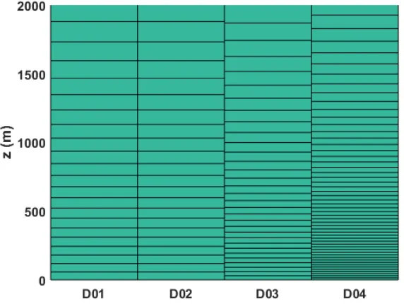
The vertical grid nesting capability [Daniels et al., 2016] implemented in WRF version 3.7

and improved in WRF version 3.8 is used here to adjust vertical resolution on each of

meters imply computational cells with very high aspect ratios when combined with a coarse

horizontal grid. These high aspect ratios cause additional numerical errors over complex terrain

due to the use of terrain following coordinates, as explained in Subsection 3.1. We use a vertical

resolution near the ground on the innermost LES domain D04 of 15 m and on the two outermost

domains D01 and D02 of 60 m. Choosing a finer vertical resolution on D04 led the simulation

to blow up. The grid spacing of the domains was increased higher aloft up to 450 m for

D01-D03 and 250 m for D04 at the top of the domain, which was placed atpht = 100 hPa. The discretization of the first 2000 m on each domain is shown in Figure 6.

Figure 6: Vertical discretization of the four domains. Only the first 2000 m above ground level is shown.

3.3

Cell Perturbation Method

The cell perturbation method was developed by Mu˜noz-Esparza et al. [2014] and improved in

Mu˜noz-Esparza et al. [2015]. The method is based on perturbations of the potential temperature,

of grid points near the inflow boundaries of the LES domain. These patches are referred to as

‘cells’. Which of the boundaries are inflow boundaries at a given moment is determined by

re-computing the average wind direction over each boundary. The perturbations are renewed

periodically after a so-called ‘perturbation time’ tp. Moreover, the random amplitude of the

perturbations in each cell is distributed uniformly over an interval [−θ˜pm,+˜θpm]. Here, θ˜pm is the maximum perturbation magnitude, determined dynamically during the simulations. The

value of θ˜pm, as well as the value of tp, is made dependent on the flow speed in a manner specified below. The method has very low computational costs and is easy to implement.

In our setup we used horizontal cells consisting of8×8 grid points. The motivation for using eight grid points is that the numerical diffusion of the WRF model dissipates energy

rapidly for k ≥ 2π/(7∆x) [Skamarock, 2004]. Therefore, any perturbation imposed with a shorter wavelength than 8∆x does not contribute much to the development of turbulence. These patches are located near the inflow boundaries of the nested LES domain; three rows

of patches parallel to the boundary are imposed, covering the first 24 grid points downstream

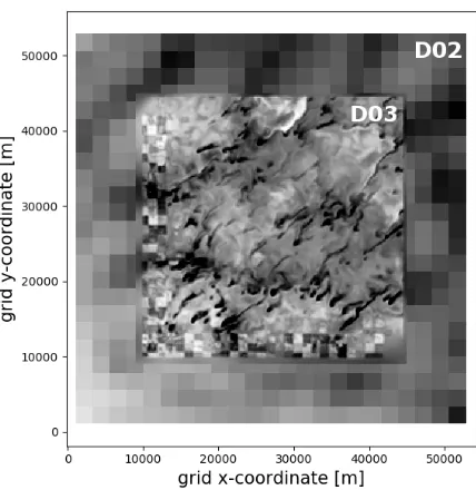
into the domain. We followed Mu˜noz-Esparza et al. [2015] in this setup. Figure 7 shows the

potential temperature field on the inner part of D02 (the outer domain with coarser grid cells)

and D03. The three rows of patches near the south and east boundaries of D03 are visible,

displaying an intermediate coarseness between the resolution of D02 and the resolution used

inside D03.

The two yet-unknown parameters in this method are the maximum perturbation magnitude

˜

θpm and the perturbation time periodtp. Following Mu˜noz-Esparza et al. [2015], we identify

two non-dimensional numbers from which these parameters can be computed: the perturbation

Eckert numberEc =U_g2/cpθ˜pmand the perturbation time-scale Γ = tpUw/dc. Here, Ug is the geostrophic wind speed,cpthe specific heat capacity at constant pressure,Uwa measure for the

Figure 7: Potential temperature field on D03 showing detailed structures, nested in D02, show-ing coarser spatial resolution. The application of CPM is easily recognized by the intermediate coarsening in 8×8 grid points at the west and south boundaries, which turned out to be the inflow boundaries at this particular instance.

cells, when traversing the cells in the direction of the local mean wind. All these four values

can be obtained during the simulations, such thattpandθ˜pmcan be computed dynamically upon selecting suitable values forEcandΓ.

The perturbation Eckert number expresses the interaction between the geostrophic forcing

and the buoyancy contribution induced by the potential temperature perturbations. CPM was

tested for different geostrophic forcings by Mu˜noz-Esparza et al. [2015] who advised an optimal

Eckert number ofEc= 0.2. This value is also used in our simulations. If the Eckert number is set too low, the perturbations are dominated by buoyancy effects and exaggerate the distortion

of the velocity field near the inflow boundaries. Moreover, the resulting strong perturbations due

to a highθ˜pmresult in rather unphysical separated high- and low-speed areas. On the other had, if the Eckert number is set too high, the effect of the imposed small-amplitude perturbations is

The perturbation time scaleΓis found by Mu˜noz-Esparza et al. [2015] atΓ = 1. The time scale describes the time that it takes to cross a cell at the ‘weakest wind’ velocity. A perturbation

time-scale lower than 1, i.e., a short perturbation time tp, results in an amplification of the

instabilities. On the other hand, settingΓ ≤ 1results in an alternating laminar and turbulent flow. As recommended by Mu˜noz-Esparza et al. [2015],Γ = 1is used. The distance across the perturbed cellsdcused inΓis computed asdc= 1/cos ( ˆφ)·24∆xwhereφˆis the average wind direction over every grid point at the inflow boundaries and the number 24 originates from three

rows of 8 grid cells.

To compute the weakest and geostrophic wind speeds, the settings of Mu˜noz-Esparza et al.

[2015] were adopted, namely setting the geostrophic wind speedUgas the horizontal wind speed

at the boundary layer heightziand the weakest wind speedUw as the horizontal wind speed at

the first grid point above the Earth’s surface, U1. Moreover, the perturbations were applied

up to2/3zi, as was recommended by Mu˜noz-Esparza et al. [2014] to avoid interference of the perturbations with the inversion layer, which could potentially trigger numerical instabilities.

However, following this original proposal, the perturbations did not accelerate the generation of

turbulence significantly. Therefore, a few adjustments were made.

Due to the very shallow boundary layer during the evening transition, the factor of2/3was increased up to 0.9, to make the perturbed region in the vertical direction larger in an attempt to

trigger turbulence also higher aloft. We did not encounter any numerical instabilities in this new

setup. To make sure that the perturbations were strong enough, the geostrophic wind speed was

evaluated at1.1ziinstead of atzi. Finally, since the wind speed at the lower three vertical levels was very low, the horizontal wind speed at the fourth grid-point above the surface was used to

evaluate the weakest wind speedUw = U4. After these adjustments a significant improvement

in the acceleration of turbulence was observed. This was used throughout the study. How the

complex terrain is interesting from a reliability perspective and will be investigated in future

research.

4

Assessment of Simulation Results using Perdig˜ao Field Data

4.1

Robustness of the Cell Perturbation Method

In this section we compare simulation results obtained with and without CPM, on small and

larger domains. CPM is designed to enrich a flow with small-scale motions only, thus the main

large-scale flow features should not be affected significantly by CPM. The goal is for CPM to

help develop turbulent flow at appropriate scales inside the domain. Hence, comparing

simu-lations without CPM, but on a larger domain with longer fetch available, with CPM enriched

simulations on a smaller domain and shorter fetch should ideally yield good similarity. Both

ver-tical velocity profiles as well as energy spectra are analyzed at verver-tical grid levelk = 8at D03, which coincides with an altitude of≈260 m AGL. The simulated date is May 9,1600−1930

LT.

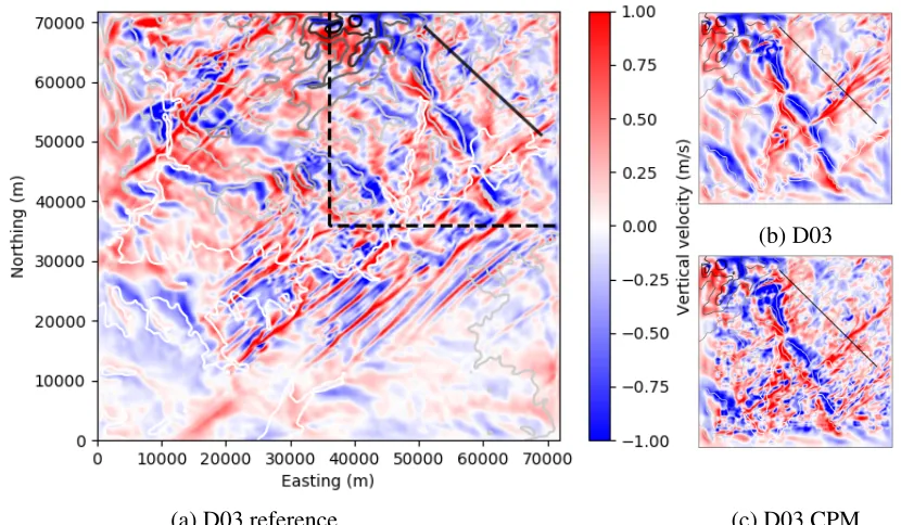
The velocity profiles in Figure 8 illustrate the robustness of global features of the simulation

results obtained for the Perdig˜ao site. As a point of reference, Figure 8(a) shows contours of

the vertical velocity over an extended domain that contains D03. CPM was not used in this

simulation - it will be referred to asD03 ref. The vertical velocity contours on the original D03

without CPM,D03, are shown in Figure 8(b) and the simulation results with CPM applied on

D03, are shown in Figure 8(c).

The simulated results are very similar in the sense that the mean flow structure, based on

the vertical velocity profile, does not change significantly. The reference simulation in Figure

8(a) shows a region of highw-velocity magnitude at and around the location of the valley. The

same structures appear in Figure 8(b). Hence, the large fetch in Figure 8(a) does not seem

(a) D03 reference

(b) D03

(c) D03 CPM

Figure 8: Vertical velocity profile at 260 m AGL at 1900 LT. Small domain without CPM (b) compared to a large reference domain without CPM (a) and small domain with CPM (c). The dashed lines in (a) show the spatial extent of the original D03. The diagonal line in (a) is used for the shown spectra comparison in Figure 9.

further smaller scale structures induced by CPM. The flow is clearly enriched with small scale

motions. Hence, CPM provides an increased control over the degree of small scales that could

be exploited to enhance the correspondence with field observations.

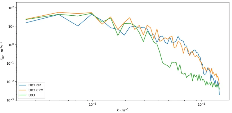
To quantify the contributions of CPM to the flow, the energy spectra of thew-velocity over

the diagonal line in Figure 8(a) across the domain D03 were computed as well. The diagonal

line contains 120 grid points and the spectra are computed following the approach of Durran

et al. [2017], averaged over five consecutive time samples with an interval of 150 seconds. The

line is located downstream of the valley such that the wind already has crossed the valley and

should be fully developed by the time it crosses the diagonal line. The results are shown in

Figures 9.

Figure 9: Comparison of energy spectra computed from the w-profile over the diagonal line shown in Figure 8(a). Averaged over five time samples, started at 1900 LT.

similar for all three simulations. However, the energy spectra for higher wavenumbers (k ≥

0.005 m−1_{) show significant differences between D03 and the other two simulations. On the}

other hand,D03 CPMshows a very similar energy spectrum compared to the spectrum ofD03

ref. This corresponds to the induced wavenumbers by CPM ofk = 2π/(8∆x) ≈ 0.005m−1. The increased agreement between results obtained on the small domain with CPM and the

reference simulation without CPM on the larger domain, nicely quantify the benefit of CPM

concerning the smaller turbulence scales, i.e., similar spectra are obtained with much less fetch.

In the next subsection we turn our attention to the influence of the domain definition on the

predicted flow.

4.2

Domain Configuration

To systematically compare the influence of different configurations of D03, simulations with

three different nested domain configurations are compared. The simulated date is the same as

of the three simulations, however, the computational grid of the domain is shifted toward the

north-east and the south-west. By doing so, we modify the distance from the domain boundary

over which the atmospheric flow can evolve within the computation domain before reaching the

valley. A shift of the nested D03 of one grid point east and one grid point south on D02 implies

a shift of 15 grid points in these directions for D03. Figure 10 shows the locations of the three

computational domains for the different setups.

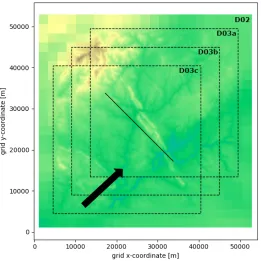
Figure 10: Location of the three different nesting setups of D03 (a-c) within D02. The vertical velocity profiles over the diagonal line are used to compare the energy spectra of the flow for the different domains. The mean flow direction is indicated by the arrow.

D03b is the default computational domain as it is defined in Figure 8(b). D03a is the same

computational domain, shifted 30 grid points to the north-east and D03c is obtained by

shift-ing D03b 30 grid points to the south-west. Four simulations are compared: three simulations

(D03a CPM). Comparison is done on the basis of energy spectra obtained from the vertical

velocity profile at 1900 LT, over the diagonal line shown in Figure 10, similar to the analysis in

Subsection 4.1. The computed spectra are shown in Figure 11.

Figure 11: Spectra of the vertical velocity profile over the diagonal line shown in Figure 10, averaged over five time samples, started at 1900 LT. Three simulations without CPM over three domains D03(a-c) and a simulations with CPM over D03a are compared.

The comparison shows a clear difference in energy spectra for the different domain

con-figurations. Spectra extracted from simulations with D03a, i.e., with a shorter distance to the

boundary in terms of the prevailing wind direction, are significantly lower. This suggests that

the turbulence levels in the flow have not developed as fully as they should in accordance to the

flow conditions. Conversely, domains with a larger distance show spectra that represent higher

energy levels for higher wavenumbers.

Similar to Figure 9, CPM clearly enriches the energy content of the smaller eddies in the

flow. In fact, the simulation with the shortest distance, but with CPM shows an energy spectrum

that compares closely with the simulation with the largest distance without CPM. The

added by the perturbations, as explained in Subsection 4.1. This clearly demonstrates the action

of CPM toward efficiently generating small-scale turbulence in a compact spatial domain.

Ap-plication of CPM can therefore be used beneficially to study turbulent flow over complex terrain

at reduced costs. Instead of having to increase the size of D03 by about 30 grid points in each

direction, one can achieve similar predictions by employing CPM at virtually no computational

overhead. In this example, increasing the grid from 241 to 271 nodes in each horizontal directly

would be an increase of 26% in computational cost.

In the next subsection the simulated results are compared to field data. The domain

configu-ration of D03b including CPM is used for the simulations to ensure a fully developed flow over

the two ridges.

4.3

Comparison to Field Data

In this subsection, the simulated results are compared to field data from the Perdig˜ao field

campaign. In contrast to the results shown in the previous two sections, the simulated results

in this section are taken from the innermost domain, D04. This domain has the highest spatial

resolution and allows for most detailed comparisons with field data. CPM is applied on both

D03 and D04 to ensure that the flow is stimulated in its development across the domain. The

simulated time is the same as before,1600−1930LT, or1500−1830UCT.

For comparison with tower data, data from eight different towers are used: rsw06, rne06,

tse13, tnw01, v06, tnw07, tse06andtse07. The locations of the towers can be found in Figure

2, Subsection 2.2. All the tower measurements are taken at 20 m AGL, except fortse13at 100

m AGL andtse06at 60 m AGL. Three different variables are compared, namely the wind speed

U, wind direction φ and the turbulent kinetic energy (TKE). The eight towers are chosen in a

specific manner to test the computational model over a range of demanding conditions. Two

wind direction, shown in Figure 12, and towers that do not line up so well, shown in Figure 13.

(a) rsw06. (b) rne06.

(c) tse13. (d) tnw01.

Figure 12: Wind direction comparison between simulated data and tower measurements taken at a ridgeline. Results in (a), (b) and (d) are measured at 20 m AGL and (c) is measured at 100 m AGL.

The towersrsw06andrne06are located at the top of the SW and NE ridgelines, respectively.

The simulated wind direction at 20 m AGL at the location of these towers in Figure 12(a)

and 12(b) show a good agreement with the measurements from the towers over the simulation

period. Figure 12(b) shows a less good agreement at the end of the time period, which could

be explained by weaker wind speeds during the evening transition. Comparison higher aloft, at

100 m AGL, with tower data fromtse13, located at the NE ridgeline, shows good agreement

throughout the entire time period. In addition to the towers on top of the ridges, the comparison

at 20 m AGL, also shows good agreement. Both the model prediction as well as the measured

results show a consistent southwesterly wind (225 degrees), as is expected from the results on

D03 shown in the previous subsections.

In contrast, Figure 13 shows the comparisons of simulations with the tower data for towers

located behind the first ridgeline, in the valley. The simulated results show an average wind

(a) v06. (b) tse06.

(c) tse07. (d) tnw07.

Figure 13: Wind direction comparison between simulated data and tower measurements taken in the valley. Results in (a), (d) and (c) are measured at 20 m AGL and (b) is measured at 60 m AGL.

direction of approximately 250 degrees with considerable variations in some places. The

mea-sured data are seen to differ significantly, with an average wind direction of 25 degrees or a

north-northwesterly wind until 1800 LT. After 1800 LT, the measured wind direction in the

of the wind direction can be explained by the influence of the ridges. The flow is possibly getting

diverted around the valley and channeled in to the valley from the north, which could explain

the northern wind measured by the towers. The model is clearly not capable of simulating this

wind shift, not at 20 m AGL (Figures 13(a), (d) and (b)), nor at 60 m AGL (Figure 13(c)).

To further compare the simulated results with tower data, the wind speed comparison for

the towers included in Figure 12 is shown in Figure 14. Despite the rather good agreement of

(a) rsw06. (b) rne06.

(c) tse13. (d) tnw01.

Figure 14: Wind speed comparison between simulated data and tower measurements taken at a ridgeline. Results in (a), (b) and (d) are measured at 20 m AGL and (c) is measured at 100 m AGL.

the simulated wind direction and the measured wind direction, the model strongly over-predicts

the wind speed at almost all the towers compared. The simulated results at the two ridges at

m/s. However, the measured data shows only a wind speed of around 10m/s. The same result is shown by the comparison higher aloft, at 100 m AGL, for towertse13in Figure 14(c). The

comparison with the towertnw01at 20 m AGL, located upstream from the SW ridgeline, shows

a smaller error, but the wind speed is over-predicted for this location as well.

The over-prediction of wind speeds near the surface is a well known problem of WRF [Ngan

et al., 2013, Jim´enez and Dudhia, 2012]. A possible reason for this over-prediction, given by

Jim´enez and Dudhia [2012], is the smoother topography used in the model. The unresolved

topographic features should produce an additional drag to the already existed drag generated

by the parameterized vegetation. An even more plausible reason for the over-prediction is the

absence of a canopy model in the simulation, which takes into account the dense vegetation of

the valley. Adding a suitable canopy model would increase the drag generated by the vegetation

as well.

The wind speed comparisons for towers inside the valley are shown in Figure 15. The

results show a better agreement of simulated results with the measurements inside the valley,

compared to the towers on top of the ridges. Especially the comparisons of the towers on the

north-side of the valley,v06andtnw07, show a good agreement with the tower data. The very

low wind speed also helps interpreting the irregular behaviour in the simulated wind directions

in Figures 15(a) and 15(d), because it is well known that the wind direction is more difficult

to predict for low wind speeds. The model over-predicts the wind speed for the towers on the

south-side of the valley, shown in Figures 15(b) and 15(c). Although all the four towers are

located inside the valley, the towers tse06 and tse07 are located closest to the SW ridgeline.

The over-prediction of the wind speed at the ridgeline could be a possible explanation for the

smaller, but still significant over-prediction at the location of the towerstse06andtse07.

To assess the generated turbulence in D04, the turbulent kinetic energy (TKE) of the

(a) v06. (b) tse06.

(c) tse07. (d) tnw07.

Figure 15: Wind speed comparison between simulated data and tower measurements taken in the valley. Results in (a), (d) and (c) are measured at 20 m AGL and (b) is measured at 60 m AGL.

turbulent fluctuationsu0_iin a turbulent flow: T KE = 1₂u0_iu0_i. The turbulent fluctuationsu0_i were obtained using Reynolds decomposition:u0_i =ui−ui, whereuiare the time-averaged velocity components. The Reynolds stress componentsu0_u0_{, v}0_v0 _andw0_w0 _{as observed in the field data}

were directly obtained from the tower-data with an interval of 5 minutes. The TKE of the tower

measurements was computed with

T KEtowers =

1 2 u

0_u0_+v0_v0_+w0_w0

(2)

To compute the TKE from the simulations, both the resolved TKE and the subgrid-scale

1.5-order TKE closure scheme and hence was available as an output from the simulation. The

resolved TKE was computed from the time seriesUi from the simulation output. The 5-minute

time average< Ui > of the time series was computed, as an approximation of time average

velocity componentsui. Using this average, the fluctuations of the time series were computed:

U_i0 =Ui−< Ui >, after which each entry of the vectorUi0 was squared. Finally, the new time seriesU_i0U_i0was averaged over a time period of 5 minutes for the period of interest (1600−1930

LC), similar to the tower data. The resolved TKE is then obtained using the same formula,

T KEsim,resolved=

1 2 U

0_U0_+V0_V0 _+W0_W0

. (3)

Due to limited storage capabilities, the output of the simulation on D04 was available at 30

second intervals and accordingly 10 samples were used to average the stress termsU_i0U_i0 and

obtain the Reynolds stressesU0

iUi0. More samples are needed to retrieve an accurate

representa-tion of the resolved TKE. However, for the eight towers considered in this secrepresenta-tion, an average

of 93% of the total TKE is contributed by the sub-grid part. Therefor we neglect the error of the

resolved TKE in this research.

The TKE comparisons between field data and simulated results for the towers positioned at

the ridgeline and upstream are shown in Figure 16. The simulated results for the locations of the

towers on the NE ridge,rne06andtse13, agree much better to the measured data, than for the

location of the tower on the SW ridge,rsw06 and the tower upstream, tnw01. The turbulence

levels induced by the flow over the valley are much higher for the locations on the NE ridge and

are seen to match the simulated results better. The simulated results for the other two towers

over-predict the TKE significantly. Moreover, all the tower comparisons show a bad agreement

for the temporal behaviour of the TKE budget.

The TKE comparison inside the valley is shown in Figure 17. The average prediction of

(a) rsw06. (b) rne06.

(c) tse13. (d) tnw01.

Figure 16: TKE comparison between simulated data and tower measurements. Results in (a), (b) and (d) are measured at 20 m AGL and (c) is measured at 100 m AGL.

general, the simulation predicts a higher TKE value with much more temporal variation than is

observed at the towers in the valley. There is a significant difference between the predictions

and the measurements of the TKE. Apparently, this quantity can not be reliably captured by the

model at this resolution, since other papers show a much smaller error, e.g., Rai et al. [2017]

and Mu˜noz-Esparza et al. [2017] show errors≤0.5m2/ss.

All the results presented in this subsection so far are generated using a model setup with

CPM on both LES domains. To quantify the influence of CPM on the accuracy of the

simula-tions, we compare the previous results generated with CPM on both LES domains with results

(a) v06. (b) tse06.

(c) tse07. (d) tnw07.

Figure 17: TKE comparison between simulated data and tower measurements. Results in (a), (d) and (c) are measured at 20 m AGL and (b) is measured at 60 m AGL.

direction and the TKE of the towertnw01are shown in Figure 18. The results do not show a

significant difference, which is expected since CPM only contributes to small scale motions,

i.e., the direction of the mean winds and the TKE should not change significantly.

The temporal behaviour for both variables in Figure 18 does change due to the CPM.

How-ever, the mean value over time of both variables stays approximately the same. The average

wind direction for the simulation without CPM is 228.6±19.8 degrees and for the simulation

with CPM 222.6±13.6 degrees. The averaged measured wind direction is 229.8 ±17.7

de-grees and hence CPM does not increase or decrease the accuracy of the simulations accordingly.

(a) Wind directionφ. (b) Turbulent Kinetic Energy.

Figure 18: Wind direction (a) and TKE (b) comparison at the location oftnw01at 20 m AGL between tower measurements and results from two simulations, one with CPM applied on two nested LES domains and one without CPM.

is 4.10±3.02 m2/s2 and for the simulation with CPM the average TKE is 3.77±2.96 m2/s2,

while the average TKE of the tower data is only 1.53±0.93 m2/s2. Hence, both simulations

are not capable of predicting the correct order of magnitude of the TKE or the prediction of the

correct temporal behaviour, as can be seen from Figure 18(b).

5

Conclusions

Nested multiscale modeling is used to represent the evening transition of May 9, 2017 at the

Perdig˜ao site in Portugal. The resolutions of the four domains ranged from ∆x = 6.75 km down to∆x = 30m. A new coupling strategy, the cell perturbation method (CPM) [Mu˜noz-Esparza et al., 2014, 2015], is implemented and adapted to the specific situation, particularly

paying attention to challenges due to the rough terrain. This is the first time that CPM is applied

to a real complex case. To that end the height up to where the perturbations are applied and the

height at which the ‘weakest’ velocity is measured were increased.

The robustness of CPM is demonstrated by comparing the results with CPM to those

struc-tures are unaltered by the method and that only the small scales are enriched. Moreover, spectra

comparisons show that these scales are enriched up to a level similar to that of the larger

do-main, suggesting that CPM successfully accelerates the development of turbulent flow in the

nested configuration.

The importance of the precise domain configuration was considered, varying the distance

from the location of the interest to the inflow boundary. Only when the spatial domain is

suf-ficiently large the flow can fully develop, implying that the smaller scales contain the correct

levels of turbulent kinetic energy. The required size of the spatial domain can be decreased

con-siderably using the cell perturbation method, suggesting savings of at least 25% in the example

configurations tested here. The energy spectra are very similar and the main flow structures are

unaltered, while the domain size is decreased significantly.

Finally, using a simulation with CPM on two nested LES domains, comparison with

ac-tual field data was undertaken. Quite good agreement of the wind direction with tower

mea-surements was found on top of the ridges. The comparisons with tower data from inside the

valley show much less good agreement. Moreover, we found that wind speed is significantly

over-predicted by the model for all the tower locations, while the turbulent kinetic energy was

observed to have about the correct order of magnitude for some of the towers, but showing a

very different temporal behaviour. For more sensitive quantities such as wind speed and TKE

the model appears to lack qualitative agreement, due to a too coarse resolution and a the lack of

a suitable canopy model.

The results from a simulation without CPM showed that the CPM did not significantly

in-crease or dein-crease the accuracy of the simulation when compared to the field observations. The

temporal behaviour of the different variables did change, but the order of magnitude stayed

approximately unaltered. A more statistical approach is needed to conclude on a possible

and TKE for simulations using higher resolution grids and a canopy model. A sensitivity

anal-yses for different mesoscale and LES closure schemes and different forcing systems such as

the European Centre for Medium-Range Weather Forecasts (ECMWF) system instead of GFS

could possibly suggest an improvement of the model configuration. Finally a sensitivity

anal-ysis for the different parameters of CPM, e.g., the height at which the weakest wind speed is

approximated and the maximum altitude up to which the perturbations are applied, might show

an improvement compared to the settings used in this research.

Acknowledgments

The major part of the research was carried out in the Environmental Fluid Mechanics and

Hy-drology group at the University of California, Berkeley in close collaboration with James M.T.

Neher and supervised by Fotini K. Chow, who both acknowledge support from the National

Sci-ence Foundation grant AGS-1565483. The author would like to acknowledge high-performance

computing support from Cheyenne (doi:10.5065/D6RX99HX) provided by NCAR’s

Computa-tional and Information Systems Laboratory, sponsored by the NaComputa-tional Science Foundation, as

well as the Savio computational cluster resource provided by the Berkeley Research Computing

program at the University of California, Berkeley (supported by the UC Berkeley Chancellor,

Vice Chancellor for Research, and Chief Information Officer). The author expresses great

ap-preciation for the members of the Environmental Fluid Mechanics and Hydrology group and

the researchers participating in the Perdig˜ao Field Campaign for their support and additionally

to Jeff Mirocha for his help with implementing the CPM code. Finally the author would like to

thank James M.T. Neher and both of his supervisors, Fotini K. Chow and Bernard J. Geurts for

References

F. K. Chow and R. L. Street. Evaluation of turbulence closure models for Large-Eddy

simula-tion over complex terrain: Flow over Askervein Hill. Journal of Applied Meteorology and

Climatology, 48(5):1050–1065, 2009. doi: 10.1175/2008JAMC1862.1.

M. H. Daniels, K. A. Lundquist, J. D. Mirocha, D. J. Wiersema, and F. K. Chow. A New Vertical

Grid Nesting Capability in the Weather Research and Forecasting (WRF) Model. Monthly

Weather Review, 144(10):3725–3747, 2016. doi: 10.1175/MWR-D-16-0049.1.

D. Durran, J. A. Weyn, and M. Q. Menchaca. Practical Considerations for Computing

Dimen-sional Spectra from Gridded Data. Monthly Weather Review, 145(9):3901–3910, 2017. ISSN

0027-0644. doi: 10.1175/MWR-D-17-0056.1.

M. J¨ahn, D. Mu˜noz-Esparza, F. Chouza, O. Reitebuch, O. Knoth, M. Haarig, and A.

Ans-mann. Investigations of boundary layer structure, cloud characteristics and vertical mixing

of aerosols at Barbados with large eddy simulations. Atmospheric Chemistry and Physics, 16

(2):651–674, 2016. doi: 10.5194/acp-16-651-2016.

P. A. Jim´enez and J. Dudhia. Improving the representation of resolved and unresolved

to-pographic effects on surface wind in the wrf model. Journal of Applied Meteorology and

Climatology, 51(2):300–316, 2 2012. doi: 10.1175/JAMC-D-11-084.1.

S. Lardeau, N. Li, and M. A. Leschziner. Large Eddy Simulation of Transitional Boundary

Lay-ers at High Free-Stream Turbulence Intensity and Implications for RANS Modeling.Journal

of Turbomachinery, 129(2):311, 4 2007. doi: 10.1115/1.2436896.

D. K. Lilly. The Representation of Small-Scale Turbulence in Numerical Simulation

Experi-ments. Proceedings of the IBM Scientific Computing Symposium on Environmental Sciences,

no. 281(November):195–210, 1967. doi: 10.5065/D62R3PMM.

Spatially-Developing Boundary Layer Simulations. Journal of Computational Physics, 140(2):233–

258, 3 1998. doi: 10.1006/jcph.1998.5882.

L. J. Mazzaro, D. Mu˜noz-Esparza, J. K. Lundquist, and R. R. Linn. Nested

mesoscale-to-LES modeling of the atmospheric boundary layer in the presence of under-resolved

con-vective structures. Journal of Advances in Modeling Earth Systems, 2017. doi: 10.1002/

2017MS000912.

J. D. Mirocha, B. Kosovi´c, and G. Kirkil. Resolved Turbulence Characteristics in

Large-Eddy Simulations Nested within Mesoscale Simulations Using the Weather Research and

Forecasting Model. Monthly Weather Review, 142(2):806–831, 2014. doi: 10.1175/

MWR-D-13-00064.1.

D. Mu˜noz-Esparza, B. Kosovi´c, J. D. Mirocha, and J. van Beeck. Bridging the Transition from

Mesoscale to Microscale Turbulence in Numerical Weather Prediction Models.

Boundary-Layer Meteorology, 153(3):409–440, 2014. doi: 10.1007/s10546-014-9956-9.

D. Mu˜noz-Esparza, B. Kosovi´c, J. V. Beeck, and J. D. Mirocha. A stochastic perturbation

method to generate inflow turbulence in large-eddy simulation models Application to

neu-trally stratified atmospheric boundary layers A stochastic perturbation method to generate

inflow turbulence in large-eddy simulation models. Physics of Fluids, 035102(035102):1–

43, 2015. doi: 10.1063/1.4913572.

D. Mu˜noz-Esparza, J. K. Lundquist, J. A. Sauer, B. Kosovi´c, and R. R. Linn. Coupled

mesoscale-LES modeling of a diurnal cycle during the CWEX-13 field campaign: From

weather to boundary-layer eddies. Journal of Advances in Modeling Earth Systems, 9(3):

1572–1594, 2017. doi: 10.1002/2017MS000960.

M. Nakanishi and H. Niino. An improved Mellor-Yamada Level-3 model with condensation

physics: Its design and verification. Boundary-Layer Meteorology, 112(1):1–31, 2004. doi:

H. Nakayama, T. Takemi, and H. Nagai. Large-eddy simulation of urban boundary-layer flows

by generating turbulent inflows from mesoscale meteorological simulations. Atmospheric

Science Letters, 13(3):180–186, 2012. doi: 10.1002/asl.377.

F. Ngan, H. Kim, P. Lee, K. Al-Wali, and B. Dornblaser. A study of nocturnal surface wind

speed overprediction by the WRF-ARW model in Southeastern Texas. Journal of Applied

Meteorology and Climatology, 52(12):2638–2653, 12 2013. doi: 10.1175/JAMC-D-13-060.

1.

R. K. Rai, L. K. Berg, B. Kosovi´c, J. D. Mirocha, M. S. Pekour, and W. J. Shaw. Comparison of

Measured and Numerically Simulated Turbulence Statistics in a Convective Boundary Layer

Over Complex Terrain. Boundary-Layer Meteorology, 163(1):69–89, 2017. doi: 10.1007/

s10546-016-0217-y.

W. C. Skamarock. Evaluating Mesoscale NWP Models Using Kinetic Energy Spectra.Monthly

Weather Review, 132(12):3019–3032, 2004. doi: 10.1175/MWR2830.1.

W. C. Skamarock and J. B. Klemp. A time-split nonhydrostatic atmospheric model for weather

research and forecasting applications.Journal of Computational Physics, 227(7):3465–3485,

3 2008. doi: 10.1016/j.jcp.2007.01.037.

J. C. Wyngaard. Toward Numerical Modeling in the Terra Incognita.Journal of the Atmospheric

Sciences, 61(14):1816–1826, 2004. doi: 10.1175/1520-0469(2004)061h1816:TNMITTi2.0.

CO;2.

B. Zhou and F. K. Chow. Nested Large-Eddy Simulations of the Intermittently Turbulent Stable

Atmospheric Boundary Layer over Real Terrain. Journal of the Atmospheric Sciences, 71(3):

1021–1039, 2014. doi: 10.1175/JAS-D-13-0168.1.

B. Zhou, J. S. Simon, and F. K. Chow. The Convective Boundary Layer in the Terra Incognita.

Journal of the Atmospheric Sciences, 71(7):2545–2563, 2014. doi: 10.1175/JAS-D-13-0356.