Symbolic Model Checking with Partitioned BDDs in Distributed Systems

(1)

M

ASTER

T

HESIS

Symbolic Model Checking with

Partitioned BDDs in Distributed

Systems

Author:

Janina T

ORBECKE

(s0191981)

Graduation Committee:

Jaco

VAN DE

POL

Wytse OORTWIJN

Ana VARBANESCU

Marieke HUISMAN

September 17, 2017

(2)

(3)

Abstract

In symbolic model checking Binary Decision Diagrams (BDDs) are often used to represent states of a system in a compressed way. By using reachability analysis the system’s entire state space can be explored. However, even with symbolic representation models can grow exponentially during an analysis such that they do not fit in a single machine’s working memory. Both multi-core and distributed reachability algorithms exist, but the combination of both is still uncommon.

In this work we present a design for multi-core distributed reachability anal-ysis. Our work is based on the multi-core model checking tool Sylvan and com-bines this with a BDD partitioning approach. As network traffic is one of the bottlenecks that are often reported in distributed reachability designs, we tried to minimize communication between machines.

(4)

(5)

List of Figures

2.1 Binary Decision Tree . . . 11

2.2 QROBDD . . . 11

2.3 ROBDD . . . 11

2.4 BDDφwith two partitions . . . 15

4.1 Flow chart of the process from the workers’ view. . . 22

4.2 Flow chart of the process from the master’s view. . . 22

4.3 Primitives commonly used in the following pseudo codes of this chapter . . . 24

4.4 Partitioned BDD . . . 30

4.5 Partitioned BDD after one reachability step . . . 33

4.6 List of new split variables . . . 35

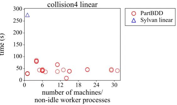
5.1 Best achieved speedup with respect to linear analysis . . . 43

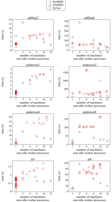
5.2 Benchmark results compared to Sylvan and DistBDD. . . 44

5.3 Final number of nodes plotted against number of active worker processes . . . 47

5.4 Execution times plotted against final number of nodes . . . 48

5.5 Communication overhead caused by idle worker processes . . . . 50

5.6 Comparision of analyses on one and four machines with final nodes 54 5.7 Comparision of analyses on one and four machines with split times 55 5.8 Execution times plotted against split count for a certain split size and number of splits . . . 57

5.9 Execution times plotted against number of splits and split count for a certain split size and number of splits (1) . . . 58

5.10 Execution times plotted against number of splits and split count for a certain split size and number of splits (2) . . . 59

(8)

(9)

Chapter 1

Introduction

In recent days the application of program verification became more important and challenging as the number of software solutions and their complexity in-creased. For instance, in the last fifty years, the size of aircraft software grew from 1.9 million lines of code (F-22) to over 24 million lines of code (F-35) [1]. One common program verification technique is model checking, where an ab-stract model of the system is built. This model can then be used to check if the software meets the requirements imposed on it.

In model checking the a program is reflected by its state space. The state space is defined as a set of all possible combinations of variable assignments in the program. Thereby the software can be seen as a graph such that com-mon graph analysis tools can be used to test for certain desired or undesired outcomes and properties. For instance, it can be tested if a certain error state is reachable from a given initial state of the system. Since verifying even small programs can result in exploring huge state spaces, several mechanisms to cope with this state space explosion problem have been developed. One method is to decrease the number of states, another is to use faster or more hardware resources.

(10)

dif-1.1. CHALLENGES FORDISTRIBUTEDMODEL CHECKING

ferent structure of BDDs compared to less restrictive graphs, in many of these cases the number of edges tends to decrease compared to the initial representa-tion. [3] By using BDD operations the state space of a system can be generated and analyzed. Although compressing the model by a symbolic representation (symbolic model checking) yields a significant reduction of states, the size of the state space remains a limiting factor.

It is also possible to use more processing units and parallelize the computa-tion. Recent work shows that a significant speedup factor of up to 38 can be reached with 48 cores by the parallel model checker Sylvan [4]. However, if the size of the model exceeds the size of the main memory, it is necessary to distribute the computation over multiple machines. Although many algorithms for distributed symbolic verification have been developed [5–8], most of them can process big models, but do not result in speedup. The main two reasons are that the computation is either executed sequentially (no speedup through par-allelization), e.g. through horizontal partitioning [6, 9], or it is slowed down due to workload or memory imbalance or communication overhead between machines. As far as we know there is only one approach that combines both multi-core and distributed architectures. This was done by Oortwijn, van Dijk and van de Pol in [10]. Their BDD package (called DistBDD) reached speedups up to 51.1 and is even able to outperform single-machine computations with Sylvan when memory runs short. [11]

In this work we focus on symbolic model checking with BDDs and the opti-mization of their distribution and processing on multiple machines. In partic-ular, we will focus on limiting communication overhead and finding a suitable BDD partitioning strategy with the goal to obtain speedups in distributed sym-bolic verification. As [11] has shown the advantages of combining multi-core with distributed algorithms, we will follow this approach.

1.1 Challenges for Distributed Model Checking

1.1.1 Locality

(11)

be-1.1. CHALLENGES FOR DISTRIBUTEDMODEL CHECKING

tween adjacent nodes are referred to ascutting edges. In a distributed environ-ment, the performance of BDD-based exploration can be improved significantly if adjacent BDD-nodes are located on the same machine such that the number of cutting edges is minimal. However, this graph partitioning problem is NP-complete [12]. There are several ways to make a good estimation of a reason-able graph distribution of explicit graphs. This operation remains challenging in symbolic reachability analysis, since it is difficult to make assumptions about the resulting graph (a BDD) obtained after applying an operation.

Obviously, locality is maximal if all nodes of the BDD belong to one ma-chine. In this case, there are no cutting edges and no communication between machines is necessary. [13] However, this is not possible in the case that the graph exceeds a machine’s memory limit. Furthermore, due to additional hard-ware resources in distributed systems, the communication overhead might be compensated by higher parallelization (load balancing).

1.1.2 Workload balancing

Together with the challenge of locality comes the issue of workload balancing. While certain problems need to be calculated sequentially, others are suited to be parallelized. For example, rendering 3D images is a task that is often performed independently for different parts of the resulting image. An exam-ple in terms of graph theory is the algorithm of Bor˚uvka which allows high parallelization of calculating the minimal spanning tree for a given graph. An optimal workload balance means that tasks are distributed over all processing units (over both machines and cores within these machines) in a way such that during a computation all these units finish processing at the same or nearly at the same time without idle or waiting times during the computation. For some types of graphs there exist approaches to achieve a good workload bal-ance while keeping the number of cutting edges low, but often a good workload balance correlates with a high number of cutting edges [14].

1.1.3 Communication Overhead

(12)

1.2. RELATEDWORK

and the more the nodes are spread over machines, the more likely it is that data must be shared between them. On the other hand, a good distribution over several machines might result in a better workload balance and therefore achieve higher parallelization of processing, which can lead to less processing time. There are graphs for which there are good distribution algorithms such that the workload is balanced and still communication is low [15]. However, in many cases it is difficult to achieve both a good workload balancing and minimal communication [13]. Still, there are also several algorithms that try to address communication overhead by sending data in bursts in contrast to continuous traffic [16] or optimize the network load in other ways [17].

1.1.4 Bandwidth/Network

Communication between machines and therefore the entire computation is also limited by the throughput/bandwidth and the latency of the used hardware of the network. Recent research indicates that the Infiniband [18] technology shows good results in this area. Infiniband supports remote direct memory access (RDMA), which decreases the latency. Therefore latency is not a bottle-neck, but the throughput is still an issue. In our opinion Infiniband is at this point the fastest and also affordable network hardware available [10, 19]. In this study we will use this technology and will not focus on finding an even better solution.

1.2 Related Work

1.2.1 Distributed Explicit Graph Analysis

(13)

1.2. RELATED WORK

were used, which are, according to the developers, essential for a balanced workload between cores. [19]

Research by Guo, Varbanescu, Epema and Iosup showed that the combina-tion of GPU and CPU resources in distributed systems can have a positive impact on the performance [20].

An explicit model checker which achieves close to linear speedup is Murφ. It uses distributed memory without synchronization between processes and a hash function to guarantee a balanced workload. [13]

Work by Inggs and Barringer on reachability analysis for CTL* model check-ing also shows nearly linear speedup. They use a shared-memory architecture with a work stealing mechanism to keep the workload balanced and minimize idle times of processors. [21]

1.2.2 Symbolic Model Checking

In 1997 Narayan, Jain, Fujita and Sangiovanni-Vincentelli invented partitioned-ROBDDs as a new way of constructing decision diagram representations for a given Boolean function. The Boolean space is divided into partitions and each partition is then represented by a ROBDD with its own variable ordering. This can result in a state space which is exponentially smaller than the generated state space using a single ROBDD. [22] According to [23] the core advantage of partitioned-ROBDDs is that for instance counterexamples in model checking can be located fast and that each partition can have its own variable ordering.

In 2000 Heyman, Geist, Grumberg and Schuster developed a partitioning algorithm with dynamic repartitioning for symbolic model checking with BDDs in a distributed-memory environment [8]. Their partitioning method (’Boolean function slicing’) is based on the work of Narayan et al. (see [22]). We will refer to it as vertical partitioning.

In 2003 Grumberg, Heyman and Schuster presented a work-efficient ap-proach due to dynamic allocation of resources and a mechanism for recovery from local state space explosion. This means that no unnecessary hardware resources are used. [17]

(14)

avail-1.3. RESEARCHQUESTIONS

able. [6]

Two years later (2006) Chung and Ciardo developed their method further and achieved speedups of up to 17 percent compared to their previous version. This time they used vertical slicing combined with speculative firing. [7]

Not a distributed technology but another way to minimize the state space are partial binary decision diagrams(POBDDs) which were developed by Townsend and Thornton in 2002 [25]. As opposed to the method of Narayan et al. not a Boolean formula but an existing ROBDD representation is partitioned into multiple partial BDDs. As far as we know this approach has not yet been used in a distributed environment.

In 2015 Oortwijn, van Dijk and van de Pol presented their findings on shared-memory hash tables for symbolic reachability model checking. They stated that for the efficient use of shared hash tables it is essential to minimize the number of roundtrips which is limited by the throughput of the network (in this case Infiniband which supports Remote Direct Memory Access – RDMA). According to Oortwijn et al. linear probing is one way to achieve less roundtrips (compared to e.g. Cuckoo hashing). With DistBDD they implemented the first BDD package that combines both distributed and multi-core reachability algo-rithms. [10, 11]

1.3 Research Questions

In the graph analysis and especially the symbolic model checking domain there are still many challenges to solve to make optimal use of the benefits of dis-tributed environments. Since in most of the cases of disdis-tributed reachability analysis the network is the bottleneck of the system, we focus in this thesis mostly on how to reduce communication overhead between machines and how to achieve this by combining existing multi-core and multi-machine approaches that have shown good performance in earlier research. We will base our work on the multi-core model checker Sylvan and the vertical partitioning method of [17].

This leads to the following main research question:

(15)

1.3. RESEARCH QUESTIONS

To better point out the different aspects, this question will be split into three sub-questions.

Subquestion 1: How can principles of vertical partitioning be combined with ex-isting multi-core model checking solutions?

Subquestion 2: How do different configurations regarding the partitioning policy affect the overall performance of the resulting system?

(16)

(17)

Chapter 2

Preliminaries on Symbolic Model

Checking

2.1 Binary Decision Diagrams

Binary decision diagrams were developed by C. Y. Lee [27] and are based on the idea of Shannon expansion [28]. Any Boolean function f can be decomposed into two sub-functions in which each Boolean variableXi is either true or false:

f(X0, . . . , Xi, . . . , Xn)≡Xi·f(X0, . . . ,1, . . . , Xn) +Xi·f(X0, . . . ,0, . . . , Xn) (2.1)

Since every variable in a Boolean formula can have two values, a binary decision tree can be built by recursively applying the Shannon expansion for-mula. Figure 2.1 is an example of such a tree. It represents formula a∨₍_b∧_c₎_.

This tree can be transformed into a directed acyclic graph (DAG) by merging or deleting some nodes. These DAGs were invented by Bryant and are called Reduced Ordered Binary Decision Diagrams (ROBDDs). [29,30]. The following definition is taken from [4].

Definition 1(Ordered Binary Decision Diagram). An (ordered) BDD is a directed acyclic graph with the following properties:

1. There is a single root node and two terminal nodes 0 and 1.

2. Each non-terminal node p has a variable label xi and two outgoing edges,

labeled 0 and 1; we writelvl(p) =i andp[v] =q, wherev∈ {₀_,₁}_.

(18)

2.2. BDD OPERATIONS

4. There are no duplicate nodes, i.e.,

∀_p∀_q·₍_lvl₍_p_{) =}_lvl₍_q₎∧_p_{[0] =}_q_[0]∧_p_{[1] =}_q_[1])→_p₌_q_.

The 0 and 1 edges are also referred to as high- and low-edges [31] and in diagrams they are indicated with dashed and solid lines respectively. A BDD that has all the properties that are mentioned in Definition 1 is called quasi-reduced (QROBDD). It does not contain duplicate nodes, but it may contain redundant nodes. These are nodes for which the node’s high and low edge lead to the same child node. A BDD which also does not contain any redundant nodes is called a reducedOBDD (ROBDD). [32]

In [4] (fully-)reduced and quasi-reduced BDDs are defined as follows:

Definition 2(Fully-reduced/Quasi-reduced BDD). Fully-reduced BDDs forbid re-dundant nodes, i.e. nodes with p[0] =p[1]. Quasi-reduced BDDs keep all redun-dant nodes, i.e., skipping levels is forbidden.

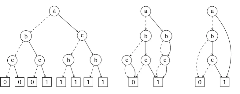
The graphs shown in Figures 2.1, 2.2, and 2.3 all describe the following Boolean formula:

a∨₍_b∧_c₎ _(2.2)

Figure 2.1 shows the decision tree belonging to the formula without any re-ductions or ordering. In Figure 2.2 all duplicate nodes of the decision tree in Figure 2.1 are removed (i.e. the two b-nodes on the bottom right) and its variables are ordered. In Figure 2.3 also the redundant nodes are removed.

In the following we refer to ROBDDs simply as BDDs.

An important part of model checking with BDDs is that there must be a unique table of nodes which is used to guarantee that there are no duplicate nodes in a BDD. This prevents the creation of superfluous nodes which may lead to overhead. In many existing implementations a hash table is used for this.

In the following section the most important operations on BDDs will be explained.

2.2 BDD Operations

(19)

2.2. BDD OPERATIONS

a

b c

c c b b

1 1 1 1

0 0 0 1

Figure 2.1: Binary Decision Tree

[image:19.595.104.497.78.233.2]

a b b c c c 1 0

Figure 2.2:QROBDD

a

b

c

1 0

Figure 2.3: ROBDD

Definition 3 (Restriction (cofactor)). Let f(x0, . . . , xn) be a BDD representing a

Boolean function and 0≤_i ≤_n_{. Then:}

restrict(f , xi,1) =fxi=1(x0, . . . ,xi, . . . , xn) = f(x0, . . . ,1, . . . , xn)

restrict(f , xi,0) =fxi=0(x0, . . . ,xi, . . . , xn) = f(x0, . . . ,0, . . . , xn)

are thepositiveandnegative restrictions(orcofactors) off with respect toxi.

Multiple BDDs can be combined in certain ways using Boolean operators like conjunction (∧_{), disjunction (}∨_{), implication (}→_{), exclusive or (}⊕_{) and more.}

Given two BDDsφandψ and a Boolean operator

op_{a new BDD} φ

op ψcan be constructed which is defined as follows:

φ op

ψ=x(φxopψx) +x

0

(φx0opψ_x0) (2.3)

The algorithm that computesφ op

ψ is based on Shannon decomposition (see Equation (2.1)) and is commonly calledapply. [33]

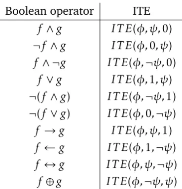
The operations computed by apply can also be expressed in an if-then-else (ITE) structure. This ITE operation is defined as follows (definition from [4]).

Definition 4 (If-Then-Else (ITE)). Let ITE_x=v be shorthand for the result of ITE(φx=v,ψx=v,χx=v) and let x be the top variable of φ, ψ and χ. Then ITE is defined as follows:

IT E(φ, ψ, χ) =

              

ψ φ= 1

χ φ= 0

(20)

2.2. BDD OPERATIONS

Boolean operator ITE

f ∧_g _{IT E}₍_{φ, ψ,}₀₎ ¬_f ∧_g _{IT E}₍_φ,₀_{, ψ}₎

f ∧ ¬_g _{IT E}₍_φ,¬_ψ,₀₎

f ∨_g _{IT E}₍_φ,₁_{, ψ}₎ ¬₍_f ∧_g₎ _{IT E}₍_φ,¬_ψ,₁₎ ¬₍_f ∨_g₎ _{IT E}₍_φ,₀_,¬_ψ₎

f →_g _{IT E}₍_{φ, ψ,}₁₎

f ←_g _{IT E}₍_φ,₁_,¬_ψ₎

f ↔_g _{IT E}₍_{φ, ψ,}¬_ψ₎

[image:20.595.195.380.85.278.2]

f ⊕_g _{IT E}₍_φ,¬_{ψ, ψ}₎

Table 2.1: Boolean operators and their ITE representation, whereφandψare the unique BDD representatives off andg, respectively.

MK(x, T , F) in Definition 4 is used to create a new BDD node with variable x. The outgoing high-edge of x goes to the BDD T and its low edge to the BDD F.

Table 2.1 shows Boolean operators and their ITE equivalents.

For a reachability analysis with BDDs there are four operations which are necessary to calculate the reachable states. These are∧_,∨_, ∃_{and substitution.}

The Boolean operators are covered by the apply operation explained above. Furthermore∧_and ∃_{are commonly combined in a single algorithm. [4]}

Listing 2.1 shows an outline of a reachability analysis, where Initial is an initial BDD, T is a BDD representing a transition relation from one state to another andXandX0 are sets of states.

1 BDD R e a c h a b i l i t y (BDD I n i t i a l , BDD T , S e t X , S e t X ’ ) 2 BDD Reachable := I n i t i a l , P r e v i o u s := 0

3 while Reachable != P r e v i o u s

4 BDD Next := (∃_X · _{( Reachable} ∧ _{T) ) [X ’ / X]}

5 P r e v i o u s := Reachable

6 Reachable := Reachable ∨ _Next

7 return Reachable

Listing 2.1: Reachability algorithm from [4]

In line 4 of the algorithm ∃_X·₍_Reachable∧_T_))[_X0_/X_] _{computes the set of}

reachable states from state Reachable using the transition relation T. After applying ∃ _{only the successors remain. This combination of}∃ _and ∧ _{is called}

the relational product (RelProd).

(21)

2.2. BDD OPERATIONS

Definition 5 (RelProd). Let X ={_x₁_{, . . . , x}_n} _and _X0 ₌ {_x0

1, . . . , x

0

n} be two sets of

variables,f :Bn→Ba Boolean function and g:Bn×Bn→Ba Boolean relation. Letφ andψ be the respective BDD representations of the functionsf and g. The relational product overφandψ with respect to X’, denoted byRelProd(φ, ψ, X, X0) is the BDD representing ∃_X·₍_f₍_X₎∧_g₍_{X, X}0₎₎_.

An example algorithm ofRelProdis shown in Listing 2.2 [4].

1 BDD RelProd ( BDD A , BDD B , Set X)

2

3 // ( 1 ) T e r m i n a t i n g c a s e s

4 i f A = 1 ∧ B = 1 then return 1

5 i f A = 0 ∨ B = 0 then return 0

6

7 // ( 2 ) Check cache , hash t a b l e f o r c o n s t a n t time a c c e s s on

8 // i n t e r m e d i a t e r e s u l t s o f BDD o p e r a t i o n s

9 i f inCache (A , B , X) then return r e s u l t

10

11 // ( 3 ) C a l c u l a t e top v a r i a b l e and c o f a c t o r s

12 x := t o p V a r i a b l e ( x_A, x_B)

13 A0 := c o f a c t o r 0 (A , x ) B0 := c o f a c t o r 0 (B , x )

14 A1 := c o f a c t o r 1 (A , x ) B1 := c o f a c t o r 1 (B , x )

15

16 i f x ∈ _X

17

18 // ( 4 ) C a l c u l a t e subproblems and r e s u l t when x ∈ _X

19 R0 := RelProd (A0, B0, X)

20 i f R0 = 1 then r e s u l t := 1 // Because 1 ∨ R1 = 1

21 e l s e

22 R1 := RelProd (A1, B1, X)

23 r e s u l t := ITE (R0, 1 , R1) // C a l c u l a t e R0 ∨ R1

24 e l s e 25

26 // ( 5 ) C a l c u l a t e subproblems and r e s u l t when x < X

27 R0 := RelProd (A0, B0, X)

28 R1 := RelProd (A1, B1, X)

29 r e s u l t := MK( x , R1, R0)

30

31 // ( 6 ) S t o r e r e s u l t in cache

32 putInCache (A , B , X , r e s u l t )

33

34 // ( 7 ) Return r e s u l t

35 return r e s u l t

Listing 2.2: RelProdalgorithm

(22)

2.3. BDD PARTITIONING

Definition 6 (Substitution). Let X = {_x₁_{, . . . , x}₂} _{be a set of variables and} _f _:

Bn → B be a Boolean function. Let x1, y ∈ X be two variables from X. Then the substitution of xi by y, denoted by f[xi ← y], is defined as f[xi ← y] ≡ f(x1, . . . , xi−₁, y, x_i₊₁, . . . , x_n). Let Y = {y₁, . . . , y_m} ⊆ X and Z = {z₁, . . . , z_m} ⊆ X

be two subsets ofX. Thenφ[Y ←_Z_]≡₍₍₍_f_[_y₁←_z₁_])[_y₂←_z₂_])_{. . .}_)[_y_m←_z_m_]_.

2.3 BDD Partitioning

2.3.1 Horizontally Partitioned BDDs

In horizontal partitioning [6, 9] the levels of a BDD are distributed over ma-chines and each level is assigned to a single machine. This means that all nodes that belong to a certain level are located on the same machine. Figure 2.4 visualizes this partitioning strategy.

1 0 w1

w2

w3

(23)

x x

1 0

φ∧_x

[image:23.595.236.377.93.281.2]

φ∧ ¬_x

Figure 2.4: BDDφwith two partitions

2.3.2 Vertically Partitioned BDDs

In [22] partitioned-ROBDDs were introduced which can be exponentially smaller than other BDDs. With partitioned-BDDs not the entire Boolean space is repre-sented as a whole, but it is divided in multiple partitions and each of them is represented by one ROBDD. The division is done using one or more “window-ing functions”w. A windowing function can be a Boolean variable or a Boolean formula, which represents a part of the BDD’s Boolean space. In Definition 7 which is taken from [22] partitioned-ROBDDs are described formally.

Definition 7(Partitioned-ROBDDs). Given a Boolean functionf :Bn→_B_defined

over Xn, a partitioned-ROBDD representationxf of f is a set ofk function pairs, xf ={(w1,f1˜), . . . ,(wk,f˜k)}wherewi :Bn→Bandf˜i :Bn→Bfor1≤i≤k, are also

defined overXnand satisfy the following conditions:

1. wi and ˜fi are represented as ROBDDs with the variable orderingπi, for1≤ i≤_k_.

2. w1∨w2∨ · · · ∨wk≡True

3. f˜i ≡wi∧f, for1≤i≤k

(24)

Research in [8, 17, 34] also uses partitioned-ROBDDs. Based on Definition 7 they developed algorithms to find suitable windowing functions for partitioning a BDD. Figure 2.4 visualizes a BDD after partitioning with windowing function

(25)

Chapter 3

Method

In the following we will describe how we try to answer the main research ques-tion and the three subquesques-tions stated in secques-tion 1.3.

To answerresearch question 1we use the work on partitioned-ROBDDs done in [34] as a starting point and try to implement their partitioning algorithm, which divides Boolean functions into multiple BDDs. These newly created BDDs can be processed locally by an existing model checker. We will use Sylvan for this purpose since this tool has shown significant speedup on multi-core ma-chines compared to other tools. In this way we hope to achieve also good speedups in a distributed environment. The goal is to extend Sylvan’s func-tionality in order to obtain communication between multiple machines within reachability analysis. This leads to several additional challenges that have to be solved like synchronization of local analyses and avoidance of unnecessary communication overhead. For communication between machines/processes we will introduce Open MPI [35], an open source implementation of the Message Passing Interface (MPI) standard [36].

(26)

3.1. VALIDATION

are interested in differences in performance (execution time) between multi-ple analyses of the same model with varying initial settings of the parameters mentioned above.

In order to find an answer to research question 3 and be able to make as-sumptions over the scalability of the system, the proposed partitioning and com-munication method, we will evaluate the system’s performance depending on the maximum size of the input model and the utilized hardware resources. In contrast to research question 2, we want to gain insights into the performance of our implementation when the initial configurations are kept the same, but the size of the input model grows. Furthermore, we are interested in how effi-ciently additional hardware resources can be used.

3.1 Validation

We will validate the implementation by executing multiple reachability anal-yses on several models. We do this with varying parameters/settings of our implementation (like the moment when a BDD is partitioned and the number of partitions that are created during partitioning). We will compare the results with those of other implementations (DistDD). Hereby we use the number of reachable states as an indication of correct calculations.

3.2 Performance Measurement

When it comes to the general evaluation of the invented method we want to be able to draw conclusions regarding its contribution with respect to the overall computation time.

To set our approach into relation with existing ones we will record and mea-sure the following factors:

• total computation time

• size of the generated state space

• number of machines that are not idle at the end of the computation (see chapter 4)

• used settings for the analysis (moment that a BDD is partitioned and num-ber of partitions that are created during partitioning)

(27)

3.2. PERFORMANCE MEASUREMENT

(28)

(29)

Chapter 4

Designing and Implementing

Distribution and Communication

Algorithm

4.1 Algorithm Overview

During reachability analysis of large models the BDD of that model might be-come too large to process on a single machine. In this case, the process can split its BDD and send one or more of its partitions to processes on other machines, if available. In this section we will give a short overview of the reachability al-gorithm we designed and implemented in this work. In the following sections, we will go into more detail.

One essential part of our design is that each analysis using our algorithm consists of at least two processes of which one is called themaster process and all other are worker processes. The master process handles part of the com-munication between processes and provides information about the progress of the analysis. The worker processes, on the other hand, are responsible for the actual reachability analysis.

(30)

4.1. ALGORITHMOVERVIEW

start

receive split vars from master

do reachability step

compute non-owned part(s)

send non-owned BDDs to and receive

owned BDDs from other workers

delete non-owned states from set of visited states

merge received BDDs with set of visited states

send status to master and receive

termination signal continue

receive BDD split from worker

receive BDD split from master

split BDD into k partitions

receive target IDs for partitions and send new split vari-ables to master

send BDD partition(s)

[image:30.595.77.499.111.404.2]

terminate

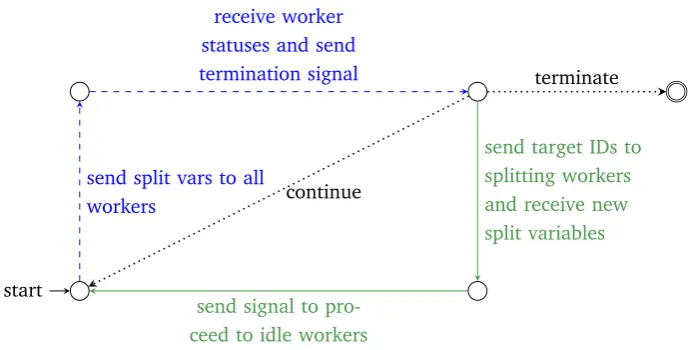
Figure 4.1: Flow chart of the process from the workers’ view. Dotted (black) arrows: local processing steps, dashed (blue) arrows: communication between a worker and the master, solid (green) arrows: communication between workers.

start

send split vars to all workers

receive worker statuses and send termination signal

continue

send target IDs to splitting workers and receive new split variables

send signal to pro-ceed to idle workers

terminate

[image:30.595.126.472.477.652.2]

(31)

from section 2.3.

Figures 4.1 and 4.2 show an overview of all the steps that each process, worker and master, perform multiple times during the reachability analysis. When the processes begin the analysis (see start node in the figures), the initial setup is already done (initializing processes, reading transition relations and initial BDD from file). The following steps are performed in each iteration:

1. Updating the list of split variables. The master process keeps track of all changes and notifies the worker processes (see section 4.5 for details).

2. Each worker process performs one level of the reachability analysis (com-putes the set of next states using the transition relation). Note that also the idle states (their local BDD is still empty, or false) do this step. Their set of next states will be empty.

3. Worker processes exchange non-owned states (see section 4.4). States that do not belong to the BDD partition of a process will be removed and states that have been received from other processes will be merged with the local BDD partition.

4. All worker processes merge their set of next states (including the received states from other processes) with all reachable states that have been ex-plored locally.

5. Each worker process determines a status (“idle”, “out of work”, “in progress”, “needs to split”) and sends it to the master process. The master process receives these messages and determines how to proceed. If all workers send the message “out of work”, the master will notify the workers to ter-minate. If at least one of the workers sent ”needs to split”, the master will handle the splitting procedure in the next step.

6. If no signal to terminate has been received, worker processes may receive or send BDD partitions. This depends on the processes’ status:

• “in progress” or “out of work”: The worker process will do nothing and continue with the next step.

• “idle”: The worker process waits for a BDD from another worker process or the master process.

(32)

multiple target processes from the master and sends the partitions to these targets. Finally it notifies the master about the used split variables.

7. The master sends empty BDDs to every process that is still idle.

Listing 4.1 gives the pseudocode to the steps described above, that runs on each worker process. Note that it is similar to the reachability algorithm in Listing 2.1 with some additional steps. On lines 7 and 16 the actual reachability analysis happens. First, the set of reachable states (Next) from the current set of already explored states (Reachable) is calculated using the relational product of the current state space and the transition relationT. Then, the states inNextare added toReachable. While the algorithm in Listing 2.1 tests whetherReachable

changes with respect to the previous iteration to terminate the while loop, our algorithm terminates, when all processes are finished. More specifically, they terminate, when the master process sends a termination signal.

On lines 9 to 15 the exchange ofnon-owned states happens. Each process sends states that it is not supposed to keep to other processes and may receive states from other processes. We explain non-owned states and their exchange in more detail in section 4.4.

The following lines of code (18 to 22) determine, if a process can receive or must send a BDD partition, does not need to do anything or has to terminate (in this case the reachability analysis is finished).

Receiving and sending of BDD partitions happens on lines 24 to 30, if any process has to split its BDD or can receive one.

Finally, each process receives updates about used split variables from the master.

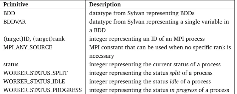
Primitive Description

BDD datatype from Sylvan representing BDDs

BDDVAR datatype from Sylvan representing a single variable in a BDD

(target)ID, (target)rank integer representing an ID of an MPI process

MPI ANY SOURCE MPI constant that can be used when no specific rank is necessary

[image:32.595.91.489.545.703.2]

status integer representing the current status of a process WORKER STATUS SPLIT integer representing the statussplitof a process WORKER STATUS IDLE integer representing the statusidleof a process WORKER STATUS PROGRESS integer representing the statusin progressof a process

(33)

4.2. SPLITTING ANDSENDING A BDD

In the next sections, we will describe each step of the algorithm in more detail.

1 // Initial BDD, transition relation T, variable sets X, X’

2 BDD R e a c h a b i l i t y (BDD I n i t i a l , BDD T , Set X , Set X ’ )

3 BDD Reachable := I n i t i a l

4 BDD S p l i t v a r s [ n u m b e r o f p r o c e s s e s ]

5 i n t q // id of this process

6 while not a l l p r o c e s s e s f i n i s h e d

7 BDD Next := (∃_X · _{( Reachable} ∧ _{T) ) [X ’ / X]}

8

9 f o r each p r o c e s s p , p , q

10 BDD n e x t s p l i t := Next ∧ _{s p l i t v a r s [ p ]}

11 s e n d t o ( p , n e x t s p l i t )

13 Next := Next ∨ _{r e c e i v e f r o m ( p )}

14

15 Next := Next ∧ _{S p l i t v a r s [ q ]}

16 Reachable := Reachable ∨ _Next

17

18 S t a t u s := d e t e r m i n e s t a t u s ( )

19 s e n d t o m a s t e r ( S t a t u s )

20 i f r e c e i v e t e r m i n a t i o n s i g n a l ( )

21 break

22

23 i f S t a t u s == SPLIT

24 i n t n := 0

25 while n < k : // k = number of partitions

26 Reachable := h a n d l e s p l i t ( Reachable )

27 n := n + 1

28 i f S t a t u s == IDLE

29 Reachable := r e c e i v e f r o m ( )

30

31 r e c e i v e a n d u p d a t e ( S p l i t v a r s )

32 return Reachable

Listing 4.1: Customized reachability algorithm

4.2 Splitting and Sending a BDD

(34)

4.2. SPLITTING AND SENDING A BDD

with the algorithm itself. Note, that we will provide details about BDD parti-tions and their creation in section 4.3. In this section we will keep this concept on a higher level. At this point it is sufficient to keep in mind, that each BDD can be split into multiple partitions. These partitions can “overlap” (are usually not disjoint) and their conjunction gives the initial BDD.

By when to split we mean: “How large is the state space of one process allowed to be?”. As a measure of the state space we use the number of nodes of the BDD. We can either choose a large number of nodes as limit, such that a BDD does just fit in the working memory of a machine. Or we can set the limit lower and split the BDD when it is smaller. The advantage of a high value is that the reachability analysis is kept on as few machines as possible. The fewer machines involved in the computation, the less time-consuming communication between them is necessary. Only when the working memory of the utilized machines does not suffice, we split and use more machines. However, splitting and sending large BDDs might consume more time compared with splitting and sending smaller BDDs. If we set the limit lower, the BDD will be split earlier. The advantage of this approach is that more machines may get involved in the computation (e.g. a BDD will be split 3 times instead of once), which can process the partitions in parallel. When a good partitioning can be found (see section 4.3) it is possible that splitting the BDD early decreases the total number of nodes (removal of redundant states). This could have an impact on the computation time. Also, splitting and sending partitions might happen faster. The disadvantage is that more communication between machines will be necessary (when exchanging non-owned states) and more duplicate nodes might be created compared with an execution with a higher maximum number of nodes.

(35)

4.2. SPLITTING ANDSENDING A BDD

of nodes. When the number of partitions is low, less machines are needed, which leads to less communication between machines. But a low split count also means that the created partitions are likely to consist each of more nodes than a partition in the case that the split count is high, because all the states of the initial BDD will be distributed over less partitions. At the same time, more partitions might lead to more duplicate nodes. We explain duplicate nodes in section 4.3. One advantage of more splits is that it might take more time until the next process needs to split, because the partitions are initially smaller. However, at the same time, creating more partitions might take longer and the communication between processes might increases.

In our implementation we use fixed numbers for the maximum number of nodes and the number of partitions per run of the algorithm. So for every partition and every split that a partition performs during the entire analysis, the same numbers are used.

Listings 4.2 and 4.3 give the pseudocode that belongs to the splitting proce-dure, the first from a worker’s point of view, the second from the master’s. As seen in Listing 2.1 on lines 26 to 28, each worker that has to split its BDD will

call handle split() k−₁ _{times, where} _k _{is the number of partitions that we}

want the worker to create.

In each iteration, the worker process will first search a suitable split variable (see section 4.3). In the next step, two partitions will be created from the BDD that contains all explored states so far. The split variable is used to generate these partitions. After this, on line 11 of Listing 4.2 and line 14 of Listing 4.3 the worker will receive a target process from the master. For this, the master iterates through all workers and chooses the first “idle” process. The worker can now send the smaller one of the created partitions to the target process which is already waiting to receive a BDD (see lines 29 and 30 in Listing 2.1). It is important that the worker keeps the larger partition, because we might want to split this one again, if the process has not yet splitk−₁_{times. In this way we try}

to achieve an even distribution of states over all created partitions. The master’s next step is to set the current status of the target process to “in progress”. This is done to avoid sending multiple partitions to that process.

(36)

4.2. SPLITTING AND SENDING A BDD

Finally, handle split returns the partition that has not been sent and the

worker process will set its BDD of reachable states to this partition.

1 BDD h a n d l e s p l i t (BDD r e a c h a b l e )

2

3 // determine the best variable to split over

4 BDDVAR s p l i t v a r := s e l e c t s p l i t v a r ( r e a c h a b l e ) 5

6 // perform the actual split and return both partitions

7 // where left is the larger part, if not equal

8 BDD r i g h t , l e f t = decompose ( r e a c h a b l e , s p l i t v a r )

9

10 // receive a “target” process from master

11 i n t t a r g e t r a n k := r e c e i v e t a r g e t r a n k ( ) 12

13 // sending smaller part of the split to “target rank”

14 bdd bsendto ( r i g h t , t a r g e t r a n k )

15

16 // send the split variables and process IDs to the master process

17 s e n d n e w s p l i t v a r s ( t a r g e t r a n k , s p l i t v a r , w o r k e r i d , neg ( s p l i t v a r ) )

18

19 // Return the other part of the splitted BDD

20 return l e f t

Listing 4.2: Pseudocode forhandle split(BDD next)

1 v o i d h a n d l e c o m m u n i c a t i o n B D D s p l i t ( )

2

3 f o r (i n t j = 1 ; j < s p l i t c o u n t ; j++)

4

5 // loop through worker processes

6 f o r each p r o c e s s p

7

8 // if p has sent worker status ‘‘has to split’’

9 i f c u r r e n t s t a t u s [ p ] == WORKER STATUS SPLIT

10 // find a worker with status ‘‘idle’’, abort otherwise 11 i n t t a r g e t i d := f i n d f i r s t i d l e p r o c e s s o r a b o r t ( ) ; 12

13 // send target id to process p

14 s e n d t a r g e t i d ( p , t a r g e t i d )

15

16 // update status of target process from ‘‘idle’’ to ‘‘in progress’’

17 c u r r e n t s t a t u s [ t a r g e t i d ] := WORKER STATUS PROGRESS

18

19 // receive new split variables from p

20 r e c e i v e s p l i t v a r s ( p )

Listing 4.3: Pseudocode for handle communication BDD split() from the master’s

(37)

4.3. FINDING THE SPLITVARIABLE

4.3 Finding the Split Variable

Whenever a worker needs to split its BDD (because it became too large), one or multiple split variables must be determined to divide the BDD into partitions. In order to generate k partitions, k−₁ _{split variables are necessary. When} _k

partitions are created, the splitting worker keeps one partition and sends k−₁

partitions to other workers. However, more than two BDD partitions are never created in a single step, but to create multiple partitions, the BDD φ (and its partitions) will be divided in two parts multiple times. For instance, when three partitions must be generated, first the initial BDD will be split along variablex. For this split variablex, one partition contains all nodes that are reachable viax

and the other partition contains all nodes that are reachable via¬_x_{. In the next}

step, one of these partitions (e.g. the¬_x_{-part) will again be split into two parts}

along variable y. This means that we now have three partitions: φ1 =φ∧x, φ2 =φ∧ ¬x∧y and φ3 =φ∧ ¬x∧ ¬y, where each has its own split function.

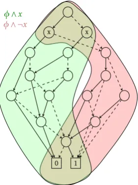
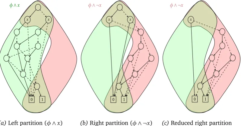
Figure 4.4 shows how two BDD partitions of the BDD given in figure 2.4 might look like.

Figure 4.4a shows the partition φ∧_x_{, which contains all BDD nodes of the}

initial BDD φ that are reachable via high (positive) edges of split variable x. Low edges of x in the initial BDD now lead to 0. Figures 4.4b and 4.4c show the counterpart of Figure 4.4a. Here, all high edges of variablex lead to0and the BDDs contain all nodes that were reachable via low edges ofxin the initial BDD φ. The BDD of Figure 4.4b is still unreduced, while in Figure 4.4c all redundant nodes are removed. In the unreduced version, both nodes on level

x have high and low edges leading to the same nodes, so they can be merged. This leads to the fact that the top node becomes redundant, because both its edges lead to the same node. This unreduced version shown in Figure 4.4b is actually never created and is included here for illustration purposes only. When BDD operations are performed on BDDs with Sylvan, the resulting BDD is kept reduced at all time and duplicate nodes are never created.

Given Figure 4.4 (especially Figures 4.4a and 4.4c) we can observe that there are many possible ways to split the initial BDD, leading to different re-sults with respect to (1) node distribution, (2) duplicate nodes and (3) node reduction:

(1) The left partition contains 11 nodes, while the right one contains 7 nodes.

(38)

x x

1 0

φ∧_x

(a)Left partition (φ∧_x)

x x

1 0

φ∧ ¬_x

(b)Right partition (φ∧ ¬_x)

x

1 0

φ∧ ¬_x

[image:38.595.87.487.103.313.2]

(c)Reduced right partition

Figure 4.4: Partitioned BDDφwith split variablex

at the bottom.

(3) The right partition could be reduced by two nodes.

Finding a suitable split variable is essential for the overall performance of the reachability analysis using vertical partitioning. An optimal split variable splits the BDD into two partitions where

1. one partition has approximately |φ_k| and the other has approximately |_φ| −

|_φ|

k nodes, where|φ|is the number of nodes in the initial BDD andkis the

number of desired partitions,

2. the number of duplicate nodes (redundancy) is as low as possible and

3. the partitions can be reduced, such that the total number of nodes de-creases.

In [8] an algorithm has been developed to find a good split variable with respect to the above criteria (see Listing 4.4). This algorithm uses the following function to determine the cost of a given partitioning of BDDφalong variablev.

cost(φ, v, α) =α∗MAX(|φv|,|φ¬v|)

|_φ| + (1−α)∗

|_φ_v|₊|_φ_¬_v|

|_φ| (4.1)

The first part, MAX(|φv|,|φ¬v|)

|_φ| , gives a measure of the reduction achieved by the partition (criterium 3), while the second part, |φv|+|φ¬v|

(39)

number of shared BDD nodes (redundancy) inφv and φ¬_v (criterium 2). The weight of both parts of the function depends on the value of α, which has to be between 0 and 1. A low α results in a low weight of the first (reduction) part and a high weight of the second (redundancy) part. As α increases, the weight of the first part increases and the weight of the second part decreases. The value ofα is reset after each search for a split variable.

Equation (4.1) only effects criterium 2 and 3, the redundancy and the re-duction of the partitioning. The partitioning algorithm (Listing 4.4), however, also takes criterium 1, the node distribution into account. First, the value of

α (which is needed in the cost function) and a step variable∆α will be set to

min(0.1,1_k), where k is the number of partitions we want to achieve. Then, on line 2, the best split variablebest var of all variablesv∈_φ_{with the given BDD}

φ and α is determined. Because α is initially low, the cost function will give most weight to the number of duplicate/shared nodes of the partitions.

At this point it may be that |_φ₁| ≈ |_φ| _and |_φ₂| ≈ ₀_{. Therefore, the split}

variable will be improved – if possible – in the following while loop (rows 3 to 5) to achieve a more balanced split. Because we want the two partitions to be of size |φ_k| and|_φ| −|φ|

k (see criterium 1), a threshold variableδis set to

|_φ|

k and will

be used in the while condition. According to [8], when the redundancy of the split is small and one of the partitions is of sizeδ, then the other partition is very likely of size |_φ| −_δ_{. From this follows that we want to find a split variable for}

which the larger partition of the split is smaller or equal to|_φ| −_δ_{. The first part}

of the while condition,max(|_φ∧_{best var}|_,|_φ∧ ¬_{best var}|₎_>|_φ| −_δ_{, checks if this}

property is fulfilled. When no such split can be found,αwill be increased by∆α

which equalsmin(0.1,0_k.1)and therefore the reduction part’s weight of the cost function increases. This will be repeated until either a suitable split variable is found or alpha becomes 1, which means that the weight of the reduction factor is maximal.

Note that although processing the while loop may take up to max(k,9) it-erations with each|_V| _{processing steps to calculate the minimum cost for each}

variable, where |_V| _{is the number of variables in} _φ_{, the total processing time}

of select var() does not increase significantly due to the while loop, because

(40)

4.4. EXCHANGINGNON-OWNEDSTATES

1 α, ∆α := min(0.1,1/k)

2 δ := |_φ|_/k

3 b e s t v a r = the variable v with minimal cost(φ, v, α)

4 while ( ( max (|φ∧ b e s t v a r|,|φ ∧ ¬b e s t v a r|) > |φ| − _δ) ∧ (α≤1) )

5 α := α +∆α

6 b e s t v a r := the variable v with minimal cost(φ, v, α)

7 return b e s t v a r

Listing 4.4: Pseudo code forselect splitvar(φ)which searches for a split variablebest var

that can be used to divide the given BDD into two partitions with desired sizes, minimal redundancy, and maximal reduction

4.4 Exchanging Non-Owned States

During reachability analysis it is very likely that a process will encounter non-owned states. These are states that belong to one or more other partitions. To define these states, we introducesplit functionswhich are essentially a single or a conjunction of multiple split variables. Every partitionφ0 of an initial BDD φ

has its own unique split function X such that the conjunction ofφand X gives the partition φ0. On the other hand, the union of all partitions exceptφ0 equals the conjunction of φand the negation of X. A more formal definition of split functions is given in Definition 8.

Definition 8(Split function). A split functionX:Bn→Bof BDD (sub-)partition φi of an initial BDD φis a Boolean function over the set of variables{x1, . . . , xn}of

BDDφ, for which

φi = φ∧X

and _ 1≤_j≤_n,

j,i

φj = φ∧ ¬X

Additionally, for every BDD φwith split function X the split functions of its par-titions φ1 = φ∧x and φ2 = φ∧ ¬x with split variable x are X10 = X∧x and X₂0 =X∧ ¬_x_{respectively.}

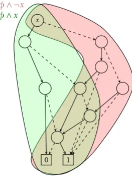
Now that we have defined split functions, we will describe non-owned states more precisely and explain why it is important that other partitions know about these states. Figure 4.5 shows an example of how the BDD from Figure 4.4c (in the following referred to as φ0) might look like after one reachability step. Ini-tially, φ0 equals φ∧_X_{, where} _φ _{is the BDD from 4.4 and} _X ₌ ¬_x _{is a split}

function to createφ0 from φ. At this point, φ0∧ ¬_X₌_false_.

(41)

4.4. EXCHANGINGNON-OWNEDSTATES

x

1 0

φ∧ ¬_x

[image:41.595.239.371.95.271.2]

φ∧_x

Figure 4.5: Resulting BDDφ0_R1after one reachability step on the partitionφ0=φ∧ ¬_x

split function,¬_X_{, is true (see the green, left part of Figure 4.5). These}

succes-sor states are called non-owned states of φ0_R₁, while states for which X is true are calledowned states.

Definition 9(Non-owned states). Letφ0be a BDD partitionφ∧_X_{of BDD}_φ_with

split functionX :Bn→B, then the non-owned states of φ0 are all states of φ0 for which¬_X _{is true. Therefore,}_φ0∧ ¬_X _{gives the BDD that contains all non-owned}

states of φ0.

With the owned states of φ0_R₁ nothing needs to happen. However, the non-owned states need to be sent to other partitions of the initial BDD, because it might be that these states could only be explored via the states in partition

φ0. On the other hand, partition φ0_R₁ might receive states for which X is true from other partitions. After all non-owned states have been exchanged, every partition will only keep their owned states and merge its received states with its own state space. For φ0_R₁ this means that φ0_R₁ := (φ_R0₁∧_X₎∨_R_{, where}_R _is

the BDD of received states. After this,φ_R0₁∧ ¬_X₌_false_and_φ0

R1∧X=φ

0

R1. How

the exchanging procedure works will be explained in the following. Note, that the set of non-owned states only needs to be computed for the newly discovered states during this iteration of reachability analysis (variableN extin Listing 2.1) and not for the entire state space ofφ0_R₁. Initially the BDD of all reachable states (Reachable) does only contain owned states. After this, only owned states will be added to this BDD, because non-owned states are removed before merging

(42)

4.5. UPDATING THELIST OFSPLITVARIABLES

We implemented the calculation and exchange of non-owned states as shown in Listing 4.5.

1 exchange non owned (BDD n e x t ) {

2 BDD r e s u l t = f a l s e ;

3

4 // send non−owned s t a t e s

6 BDD o t h e r ;

7

8 // determine p a r t s owned by worker p by u s i n g t h e s p l i t

9 // f u n c t i o n o f p

10 i f ( s p l i t f u n c t i o n s [ p ] == t r u e )

11 o t h e r = f a l s e ;

12 e l s e

13 o t h e r = n e x t ∧ _{s p l i t f u n c t i o n s [ p ]}

14

15 // send non−_{owned p a r t s t o p r o c e s s p w i t h o u t w a i t i n g}

16 // f o r p t o r e c e i v e t h e message

17 b d d i b s e n d t o ( o t h e r , p )

18

19 // r e c e i v e owned s t a t e s from o t h e r workers

21 BDD tmp = bdd brecvfrom (ANY SOURCE) ;

22 r e s u l t = r e s u l t ∨ _{tmp ;}

23

24 // w a i t u n t i l a l l non−_{owned s t a t e s have been}

25 // r e c e i v e d by o t h e r p r o c e s s e s

27 w a i t u n t i l r e c v ( p ) ;

28

29 return r e s u l t ;

Listing 4.5: Pseudocode forexchange nonowned(BDD next)

4.5 Updating the List of Split Variables

Every process that is involved in the reachability analysis has a local list of split variables or split functions, stored as BDDs. For each entry in this list, also the ID of the process is stored which a specific split function belongs to.

Every time when new BDD partitions have been created, this list of split variables has to be updated. In order to minimize the communication that is needed to update all lists, the processes are only notified about the variables that have changed, or more specific, have been added to a split function. This happens according to a specific protocol.

(43)

4.5. UPDATING THELIST OFSPLITVARIABLES

to generate the partitions and also its own and the target process ID to the master. The master receives a list of four entries (target ID, split variable target ID, worker ID, split variable worker ID – in this order) for every split that a process does. It stores all lists that it receives during one reachability step in a larger list. In the end of each reachability step the master sends this list to each process (see line 33 of Listing 4.2). Figure 4.6 visualizes the design of the list that the master sends. The gray boxes on top of the list indicate which entries belong to one split and which process sent the information. These are not stored by the master but are only shown for clarification purposes.

process 2 process 1

split 1 split 2 split 3

[image:43.595.111.505.258.334.2]

t id t sv s id s sv t id t sv s id s sv t id t sv s id s sv . . .

Figure 4.6: List of new split variables

The length of the list that the master sends is always a multiple of four. The processes receive this list and add the new split variables to their local list of split variables (L) as follows:

For each set of four elements

• Read the target process ID (t id)

• Read the target split variable (t sv) and transform it into a BDD (target BDD).

• Merge the target BDD with the current entry for the target ID in L and store the result as the new split BDD of the target process (L[t id] =

L[t id]∧_{target BDD).}

• Read the source process ID (s id).

• MergeL[t id] with the current entry for the source ID in L and store the result as the new split BDD of the target process (L[t id] = L[t id] ∧

L[s id]).

(44)

4.6. DETERMINING THESTATUS AND TERMINATION

• Merge the source BDD with the current entry for the source ID in L and store the result as the new split BDD of the source process (L[s id] =

L[s id]∧ _{source BDD).}

Due to the fact that the process with the target ID has received a partition from the process with the source ID, its received partition will only contain states that have been in the BDD of the target process before the split. These are states for which L[s id] is true. This is why the split function of the target process (before the split) has to be merged with the split variable (or split BDD) that is used to create the target’s partition.

4.6 Determining the Status and Termination

In each iteration the master process has to determine if all processes are fin-ished with their calculation, if some are still running or if a BDD needs to be partitioned. To be able to do this, every worker sends his status to the master once in each iteration. We chose to use four statuses for this purpose:

1. idle

2. out of work

3. in progress

4. needs to split

(45)

4.7. IMPLEMENTATIONDETAILS

BDD partition, given that the split happens only when a BDD does not fit in a single machine’s working memory any more.

The third status, in progress, means that a process has explored new states and its state space is still smaller then the maximum number of allowed nodes. When a worker has the fourth status, needs to split, he has discovered new states and the size of its BDD exceeds the maximum number of allowed nodes. This status signals the master that it has to perform additional actions in the next step such as sending target process IDs for BDD partitions to the worker.

After all processes have sent their statuses, the master determines an overall status and sends a signal to continue or terminate back to the processes. There are three outcomes:

• At least one process sent needs to split: Notify workers to continue. Han-dle splitting procedure in the next step. Abort if no iHan-dle process is left. Otherwise, if

• at least one process sent in progress: Notify workers to continue. Analysis is not done, yet. Otherwise,

• all processes sent either idle or out of work: Notify workers to terminate. The analysis is done.

4.7 Implementation Details

In this section we will provide some information about our implementation of the algorithm described above.

In our implementation we combined locally running versions of Sylvan with a BDD partitioning approach. For this, we tried to reuse as much code from Sylvan as possible. With respect to the splitting procedure there was no ex-isting code that we could base our implementation on. This is why we have implemented this part from scratch. As the communication interface between processes we used MPI, the Message Passing Interface. One advantage of MPI is that it can handle communication between processes on one machine as well as communication between processes on different machines without the need to change any of the code.

Symbolic Model Checking with Partitioned BDDs in Distributed Systems

M

ASTER

T

HESIS

Symbolic Model Checking with

Partitioned BDDs in Distributed

Systems

Author:

Janina T

(s0191981)

Graduation Committee:

Jaco

POL

Wytse OORTWIJN

Ana VARBANESCU

Marieke HUISMAN

September 17, 2017

Abstract

Contents

List of Figures

Chapter 1

Introduction

1.1

Challenges for Distributed Model Checking

1.1.1

Locality

1.1.2

Workload balancing

1.1.3

Communication Overhead

1.1.4

Bandwidth/Network

1.2

Related Work

1.2.1

Distributed Explicit Graph Analysis

1.2.2

Symbolic Model Checking

1.3

Research Questions

Chapter 2

Preliminaries on Symbolic Model

Checking

2.1

Binary Decision Diagrams

2.2

BDD Operations

2.3

BDD Partitioning

2.3.1

Horizontally Partitioned BDDs

2.3.2

Vertically Partitioned BDDs

Chapter 3

Method

3.1

Validation

3.2

Performance Measurement

Chapter 4

Designing and Implementing

Distribution and Communication

Algorithm

4.1

Algorithm Overview

4.2

Splitting and Sending a BDD

4.3

Finding the Split Variable

4.4

Exchanging Non-Owned States

4.5

Updating the List of Split Variables

4.6

Determining the Status and Termination

4.7

Implementation Details