University of Warwick institutional repository:http://go.warwick.ac.uk/wrap
A Thesis Submitted for the Degree of PhD at the University of Warwick
http://go.warwick.ac.uk/wrap/57735
This thesis is made available online and is protected by original copyright. Please scroll down to view the document itself.
The Valuation of Exotic Barrier Options and
American Options using Monte Carlo Simulation
by
Pokpong Chirayukool
Thesis
Submitted to the University of Warwick
for the degree of
Doctor of Philosophy
Warwick Business School
September 2011
Contents
List of Tables v
List of Figures viii
Acknowledgments x
Declarations xi
Abstract xii
Chapter 1 Introduction 1
I
Contour bridge Simulation
4Chapter 2 Literature Review on Barrier Options and Hitting Times 5
2.1 An overview of barrier options . . . 5
2.2 Valuation of barrier options . . . 7
2.2.1 Valuation methods with GBM and constant barrier. 7
2.2.2 Non-GBM processes .
2.2.3 Non-constant barriers
2.3 Hitting times . . . .
2.3.1 Zt is a Brownian motion
2.3.2 Zt is a non-Brownian motion
2.4 ConcI us ion . . . .
Chapter 3 Valuing Exotic Barrier Options using the Contour Bridge
13
16
18
19
20
21
Method 22
3.1 Simulation methods for barrier options. . . . 23
3.1.1 Dirichlet Monte Carlo method . . . . 23
3.2 The contour bridge simulation method 26
3.2.1 The choice of contour
...
273.2.2 Hitting time sampling method 29
3.2.3 The contour bridge method algorithm 35
3.2.4 The stopping conditions . . 37
3.2.5 Computing the value of ST 40
3.2.6 Single-hit method barriers. 42
3.2.7 The biggest-bite variant
..
433.2.8 The vertical contours variant 44
3.2.9 Valuation of a book of options 44
3.3 Numerical results . . . 45
3.3.1 The benchmark option. 46
3.3.2 The exotic options 51
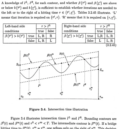
3.3.3 Numerical results. 53
3.4 Conclusion
...
64II American Put Options and Control Variates 65
Chapter 4 Literature Review on American Option Valuation 66
4.1 American put option valuation problems. 66
4.2 Approximation and numerical methods. . 68
4.2.1 Analytical approximation methods 68
4.2.2 PDE and lattice methods 70
4.3 Simulation methods . . . 71
4.3.1 Mesh methods . . . 72
4.3.2 State-space partitioning methods 74
4.3.3 Duality methods . . . 76
4.3.4
4.3.5
4.3.6
Functional form methods . . . .
Overview of the control variate method
Control variate method for American option valuation
4.4 American option valuation in stochastic volatility, Levy and jump processes, and stochastic interest rate models
4.4.1 Stochastic volatility . . .
4.4.2 Levy and jump processes ..
4.4.3 Stochastic interest rate. . . .
4.5 American barrier and power options
4.5.1 American barrier . . . .
77
80 82
4.5.2 Power option
4.6 Conclusion . . .
90
90
Chapter 5 Valuing Bermudan and American Put Options with
Bermu-dan Put Option Control Variates 92
5.1 Exercise at fixed times: Bermudan options. . . 93
5.2 Bermudan option control variate . . . 93
5.2.1 Bermudan put-terminal control variate.
5.2.2 Bermudan put-tau control variate ..
5.2.3 Obtaining values of Tj from simulation.
5.3 Two-phase simulation method . . . .
5.3.1 First phase: Estimating the early exercise boundary
5.3.2 Second phase: Computing the option value . . . . .
96 97 100 100 100 103 5.4 Approximate American put options using Richardson extrapolation. 105
5.4.1 Two-point scheme . . . 105
5.4.2 Three-point scheme . . . 106
5.4.3 Implementing Richardson extrapolation with Monte Carlo and
control variates . . . 5.5 Numerical results . . . .
5.5.1 First phase results .
5.5.2 Second phase results
5.6 Conclusion . . . .
Chapter 6 Valuing American Put Options using the Sequential
Con-107
108
109
110
119
tour Monte Carlo Method 121
6.1 The sequential contour Monte Carlo (SCMC) Method 121
6.1.1 Sequential contour (SC) options . . . 123
6.1.2 Sequential contour path construction. . . 124
6.1.3 The SCMC algorithm: the generalisation of the LSLS algorithm129
6.1.4 Using SC put options to approximate American put options:
Richardson extrapolation
6.2 Sequential contour construction . . . .
6.2.1 Choice of gN-I . . . • . • . 6.2.2 Choices of aD, aN-I, and gi,i = 1, ... ,N - 2
6.3 Control variates from the SCMC method . . . .
6.3.1 6.3.2
6.3.3
Valuing barrier options by using hitting time simulation
Hitting times and options . . . .
Rebate options from the SCMC method
6.4
6.3.4 Rebate option control variate Numerical Results . . . . 6.4.1 Choice of contours . . . .
6.4.2 Early exercise boundary of sequential contour options
6.4.3 Valuing standard American put options
139 140 140 143 144 6.5 Conclusion . . . 153
III
Projection Techniques and Exotic American Options 154Chapter 7 Valuing Exotic American Options using the Sequential
Contour Monte Carlo Method 155
7.1 Sequential contour bridge (SCB) method. . . 156
7.1.1 Contour construction for the SCB method. 156
7.1.2 The SCB algorithm . . . 158
7.2 Different projection techniques . . . 158
7.2.1 Generalised LSLS Algorithm with projection operator 160
7.2.2 Hitting times projection (T-projection) . . . . 161
7.2.3 Contour distance projection (V-projection) . . . 162
7.3 Application to American fractional power call options . . . . 163
7.3.1 Valuation of an American fractional power call option 164
7.3.2 Contour construction for an American fractional power call option . . . 166 7.4 Application to American linear barrier fractional power call options. 169 7.5 Numerical Results . . . " 172
7.6
7.5.1 Sequential contour bridge (SCB) method with American put options . . . .
7.5.2 American fractional power call option results .. . 7.5.3 American knock-in option results . . . . 7.5.4 Benchmark options: flat barrier with power K,
=
1 7.5.5 Exotic American options.Conclusion . . . .
Chapter 8 Conclusion
173
177
179 179 180 185
187
Appendix A The derivation of the hitting time bridge distribution 192
List of Tables
2.1 Examples of T-option and L-option . . . .
3.1 Benchmark valuation, rebate, fiat barrier. (J' = 0.1
3.2 Benchmark valuation, rebate, fiat barrier. (J' = 0.2
3.3 Benchmark valuation, rebate, fiat barrier. (J' = 0.3
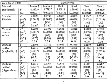
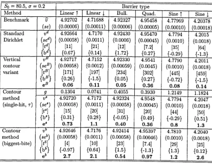
3.4 Exotic barrier types and parameters
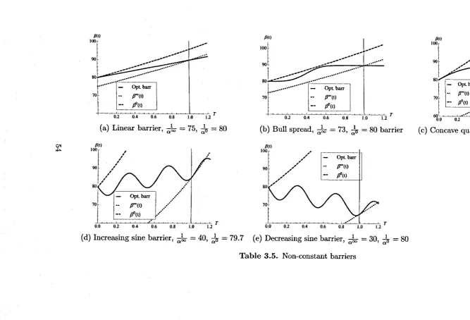
3.5 Non-constant barriers . . .
3.6 Rebate option OR, (J' = 0.2 . . . .
3.7 Knock-in call option OIC, (J' = 0.2
3.8 Knock-in put option OIP, (J' = 0.2
6
48
49
50
53
54
55
55
56
3.9 Recovery option orec, (J' = 0.2 . . . 56
3.10 Knock-in call option OIC and knock-out put option ODP, single-hit
[" (J' = 0.2 . . . 58
3.11 Rebate option OR, close to the barrier, (J' = 0.2 . . . . 59
3.12 Knock-in call option OIC, close to the barrier, (J' = 0.2 59
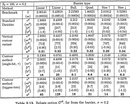
3.13 Rebate option OR, far from the barrier, (J' = 0.2 . . . . 60
3.14 Knock-in call option OIC, far from the barrier, (J' = 0.2 . 60
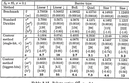
3.15 Rebate option OR, (J' = 0.1 62
3.16 Knock-in call option OIC, (J' = 0.1 62
3.17 Rebate option OR, (J' = 0.3 . . . . 63
3.18 Knock-in call option OIC, (J' = 0.3 63
5.1 Four cases of the Bermudan put control variate, cb2 • 97
5.2 Laguerre polynomial characteristics. . . .. 102
5.3 RMSEs comparison between the put-tau,
cJ;.,
and a combination ofthe put-tau and the Bermudan put-tau,
cJ;.+b2,
rollback method . .. 109 5.4 Summary of control variates used in table 5.5 . . . .. 1115.5 Bermudan put values and variance reduction gains from various kinds
5.6 Two-phase method to value Bermudan put options. Put+Bermudan
tau roll back with So-dispersion. Pricing control variates are put-tau
and put-tau + Bermudan early. Benchmark price is 4.00646. 114
5.7 Two-phase method to value Bermudan put options. X = 100. Bench-mark value is 6.08118. . . .. 115
5.8 Two-phase method to value Bermudan put options. Benchmark value
is 8.72811 . . . .. 116
5.9 Extrapolated American put values with pricing control variate only. 118
5.10 Extrapolated American put values with pricing and v(O) control variate118
5.11 Efficiency gains from adding v(O) control. . . . 119
6.1 T-modified path illustration, T = 1 and N = 6 6.2 Summary of SC option types . . . .
6.3 Options defined by hitting times . . . .
6.4 Extrapolated American put values from type 4 SC option with
dif-ferent values of kmax and kmin . ;1N-l(O) = 5 and gN-l = 2.99. 127
132
137
Benchmark value is 6.09037 . . . " 142
6.5 Contour parameter values . . . .. 142
6.6 Extrapolated American put option values from the SCMC method
with different types, a = 0.2 . . . 143 6.7 Extrapolated American put values from SC option values without the
v(O) control . . . 145 6.8 Extrapolated American put values from SC option values with v(O)
control. . . .. 147
6.9 Correlations between extrapolated American put and v(O) controls,
p
(VOO, :uN) . . . . . . . . . . . . . . . . . . . ..
148 6.10 Extrapolated American put values from the sequential contourop-tions with only pricing control. . . .. 151
6.11 Extrapolated American put values from the sequential contour
op-tions with pricing and v(O) control . . . .. 152
7.1 Comparison of American and European fractional power call options 163
7.2 American fractional call values with different ;1N-l(T) . . . . 167 7.3 American put, a
=
0.2 . . . .. 174 7.4 Bias in extrapolated American put values using T-projection . . .. 1767.5 American fractional power call option with forward evolution
7.6 Benchmark case: knock-in flat barrier American call options with
fi, = 1. . . .. 181 7.7 Knock-in linear barrier fractional power American call options, So =
105 . . . .. 182
7.8 Knock-in linear barrier fractional power American call options, So =
100 . . . .. 183
List of Figures
3.1 Illustration of a bridge hitting time 701
I
7011, 70123.2 Hitting time densities where v
>
0 and v<
0 3.3 Contour bridge algorithm illustration . . . .28
32
37
3.4 Intersection time illustration. . . 39
3.5 Bimodal bridge hitting time density;
f
(701I
7011, 7012 ). 7011 = 0.25,7012 = 0.26, 2-. = 70.2, .!. = 70, 2-. = 69.8 . 41
011 01 012
3.6 Biggest bite illustration . . . 44
4.1 American put option's early exercise boundary (EEB) 68
5.1 Convergence of a Bermudan option value to an American option value
from a trinomial lattice method . . . 94
5.2 A B-spline defined by a set of knot points {O, 2, 4, 8, 16} 104
6.1 Bermudan and SC option's exercise opportunities. 125
6.2 Illustration of path construction. . 126
6.3 Iteration of the SCMC algorithm . . . 130
6.4 The four types of sequential contours . . . 135
6.5 Asset value simulation from the SCMC method 136
6.6 Contour shape with different kmax and kmin • N = 50, ,aN-l(O) = 5
and gN-l = 2.99. . . . 141 6.7 Early exercise boundaries of the sequential contour puts and the
American put . . . .. 144
6.8 Convergence of SC put option values to American put values for
var-ious
So . . . ..
146 6.9 Correlations between c:·i with1)64,
their covariances, and standarddeviations for different contours ,ai(t) . . . . . 149
7.2 Convergence of Bermudan fractional call option values to the
Amer-ican value from a lattice method .. . . . 165
7.3 American fractional power call options' EEB 166
7.4 Contour construction for an American fractional power call with its
EEB from Richardson extrapolation . . . " 168
7.5 The values of ST (area (a), (b) and (c)) . . . " 169 7.6 Continuation values, regression values and exercise values from the
S-projection and the T-projection method, for a SC put option, on
the 62th contour . . . .. 175
7.7 Continuation values, regression values and exercise values from the
T-projection method, for a SC fractional call option, on the 62th
contour . . . . 179
Acknow ledgments
I would like to first show my gratitude to my supervisor, Dr. Nick Webber, for
his continual supports, advices, detailed comments, and patience for the past four
years. I have learnt a lot from him. This thesis would not have been completed
without his help.
I am truly indebted to my parents, Mrs. Vipada and Mr. Jitti Chirayukool
for their encouragements, understandings and financial supports throughout my
study. Thanks are due to them for giving me an opportunity to pursue this PhD. I
could not have finished this thesis without them.
Many thanks go to Ms Somsawai Kuldiloke for always being encouraging,
considerate, and supportive. I deeply thank her for being an excellent listener.
Declarations
I hereby declare that this thesis is the result of my original research work and effort.
When other sources of information have been used, they have been acknowledged.
Abstract
Monte Carlo simulation is a widely used numerical method for valuing
fi-nancial derivatives. It can be used to value high-dimensional options or complex
path-dependent options. Part one of the thesis is concerned with the valuation of
barrier options with complex time-varying barriers. In Part one, a novel
simula-tion method, the contour bridge method, is proposed to value exotic time-varying
barrier options. The new method is applied to value several exotic barrier options,
including those with quadratic and trigonometric barriers.
Part two of this thesis is concerned with the valuation of American options
using the Monte Carlo simulation method. Since the Monte Carlo simulation can
be computationally expensive, variance reduction methods must be used in order
to implement Monte Carlo simulation efficiently. Chapter 5 proposes a new control
variate method, based on the use of Bermudan put options, to value standard
Amer-ican options. It is shown that this new control variate method achieves significant
gains over previous methods. Chapter 6 focuses on the extension and the
generalisa-tion of the standard regression method for valuing American opgeneralisa-tions. The proposed
method, the sequential contour Monte Carlo (SCMC) method, is based on hitting
time simulation to a fixed set of contours. The SCMC method values American put
options without bias and achieves marginal gains over the standard method. Lastly,
in Part three, the SCMC method is combined with the contour bridge method to
value American knock-in options with a linear barrier. The method can value
Chapter
1
Introduction
Barrier options are well-known exotic options that are traded in the market. They
are popular among investors since they are cheaper than the corresponding European
options and they can be used to gain or to reduce an exposure. They also occur
in debt instrument and arise in credit risk application. Although there are several
standard valuation methods that can be used to value barrier option accurately,
these methods often work when the shape of the barrier is simple such as a flat or
an exponential barrier, and can value only a single option at a time.
The more complex versions of barrier options are characterised by conditional
or non-constant barriers. Even though standard simulation methods can be used
to value these complex options, they are often slow and prone to simulation biases.
The first part of this thesis is concerned with the development of a novel simulation
method to value complex-shape barrier options accurately and to improve on the
standard simulation method in term of computational costs.
American options and American style derivatives have become one of the
most common financial instruments traded both in exchange and in the over-the-counter market. These types of options are difficult to value because of their early
exercise feature. This special feature of American options complicates the pricing
problem because one needs to solve for the exercise boundary simultaneously with
the option value. The standard Black-Scholes partial differential equation (PDE)
becomes a free boundary value problem. Because in several settings partial different
equation (PDE) methods may be numerically difficult to use, Monte Carlo
simu-lation can be used as an alternative numerical method to price American options.
However, Monte Carlo simulation can be computationally expensive. Therefore,
variance reductions techniques must be used in order to implement Monte Carlo
a new simulation method to value standard and exotic American options are the
main focus of part two and part three of the thesis.
There are three main contributions of this thesis. The first contribution is
the development of a novel simulation method, based on a hitting time simulation,
to value exotic barrier options and to improve upon the standard simulation method.
The second contribution is the development of a new control variate technique, based
on the use of a Bermudan option, to value Bermudan and American put options.
The new control variate method can be used to reduce substantially computational
costs of a simulation method. The third contribution is the extension and the
generalisation of the standard Least Squares Monte Carlo method of Longstaff and
Schwartz (1995) [177] (LSLS) to value standard and exotic American options.
Throughout this thesis, the time t asset value St is assumed to follow the geometric Brownian motion. That is,
(1.0.1)
where Zt is a Brownian motion, r is a risk free rate and (J' is volatility. A risk free rate and volatility are assumed to be constant.
At the beginning of the thesis, Chapter 2 provides a literature review of
valuation methods that have been used to value barrier options. It also provides a general review of the hitting time, a concept that is crucial to the barrier option
valuation problem and the development of the new simulation technique.
In Chapter 3 of the thesis, the novel simulation method, the contour bridge method, is introduced and is described. The method is applied to the valuation of
exotic barrier options. Several complex non-constant barrier options are introduced.
These range from a not very complicated linear barrier option to a more complex
trigonometric-shape barrier option. The method is based on a hitting time simula-tion and a bridge hitting time simulasimula-tion to a specific type of contour. Numerical
results show that biases in resulting barrier option values are negligible and most
of the time the contour bridge method achieves substantial efficiency gains over
standard simulation methods.
Part two of the thesis begins by reviewing existing American valuation
meth-ods. Chapter 4 reviews semi-analytical and numerical methods used in valuing
stan-dard American options both in the geometric Brownian motion model and in other
models. The chapter also reviews the valuation of American options by using
sim-ulation techniques. Different simsim-ulation methods are reviewed and described. The
variate techniques for valuing American options are reviewed and discussed. The
chapter lastly describes the pricing of American barrier options and a power option;
the two options that will be considered in the last part of the thesis.
In Chapter 5, a new control variate technique is proposed. The new method
makes use of the twice-exercise Bermudan put option as a control variate. The
Bermudan control variate is implemented to value Bermudan put options using a
two-phase Monte Carlo simulation method. The results suggest that the Bermudan
control variate method gives accurate values for Bermudan options and achieves
significant efficiency gains over the plain LSLS method. It is also shown that Amer-ican put option values can be approximated accurately by employing the three-point
Richardson extrapolation method. The standard errors of an extrapolated
Amer-ican value are also reduced by using a value of an individual Bermudan put as a
control variate.
Chapter 6 extends and generalises the standard LSLS method for valuing
American put options. The new method, the sequential contour Monte Carlo
(SCMC) method, simulates hitting times to a fixed set of exponential contours.
The method generalises the LSLS method to a more general family of contours and
instead of iterating backward on a fixed time step, the method iterates backward
on each contour with a varied time step. It is shown that sampled hitting times to contours can be used to value barrier options and these options can be used as
control variates. Numerical examples show that the method can value American
put options without evidence of bias and it achieves marginal efficiency gains over
the standard method.
Chapter 7 extends the SCMC method by introducing two new projection
techniques to approximate an option's continuation values. The new techniques are
the T- and the V-projections. These techniques are applied to value American put and American fractional call options. The second part of Chapter 7 demonstrates
the application of these techniques to value exotic American options; the American
linear knock-in fractional power call option. To value this option, the SCMC method
is modified by incorporating the contour bridge method introduced in Chapter 3.
The method can value American knock-in options without any evidence of bias and
also achieve respectable efficiency gains over the standard LSLS method.
Lastly, Chapter 8 presents the conclusion and observations of the complete
thesis. Recommendations for future research are pointed out. There is an appendix
consisting of two parts. The first part is concerned with the derivation of the bridge
hitting time density that is used in Chapter 3. The second part shows the derivation
Part I
Chapter
2
Literature Review on Barrier
Options and Hitting Times
Barrier options have become popular exotic options that are traded in the market. They enable investors to avoid or obtain the exposure and they are cheaper than
the corresponding European options. They can be monitored either continuously or
discretely. There are explicit solutions for barrier options for a simple case; single or
double constant barriers with single underlying asset that follows a geometric
Brow-nian motion process in (1.0.1). For a more complicated barrier option or process,
numerical methods must be used. A concept that is closely related and is important
to barrier options is that of a hitting time. It is the first time that a stochastic process crosses a certain barrier level. The hitting time has been used in several
applications in option pricing such as the valuation of barrier options and American options.
This chapter provides an overview of barrier options, their valuation methods
and hitting times to several types of barrier. An overview of barrier options is
discussed in section 2.1. Section 2.2 reviews several valuation methods for barrier
options. The review of hitting times is provided in section 2.3.
2.1
An overview of barrier options
Barrier options are a modified form of standard plain-vanilla European options. The
payoff of barrier options depends on whether or not an asset value hits a pre-specified
barrier level during the life of an option. An in-option will payout only if an asset
value crosses a barrier. On the other hand, an out-option will payout only if an
value at time
to
is above the initial value of the barrier, an option is referred to as a down-option. If the initial asset value is below the timeto
value of the barrier, an option is referred to as an up-option. A barrier option can have either single ordouble barriers.
Let b(t), t E [0, T] be a barrier level at time t for a barrier option maturing at time T and St be an asset value at time
t.
If a barrier is constant, one writesb(t)
==
b. Write T for the first hitting time of S = (St)t~O to the option barrier. Thefirst hitting time for a barrier option is defined as
T
=
min{t E[0,
T] : St=
b(t)}. (2.1.1)Let /, = llr:::;T, where llr:::;T is the indicator function, be a variable determining whether or not the barrier is hit before time T. Barrier options can be categorised into two main groups. The first group is an option whose payoff depends directly
on T. The second group is an option whose payoff depends on T only through /"
The former is referred to as a T-option and the latter is referred to as an /'-option.
There is also a special case of an /'-option called a bare-/, option. Examples are
shown in table 2.1. Usually, to value an /,-option, one needs to compute additional
Type Example
T-option rebate option, paying at T
/,-option knock-in option
knock-out option
bare-/, option knock-out option, paying rebate at T
Table 2.1. Examples of T-option and /,-option
quantity such as the asset value of maturity time T, ST, to compute an option's payoff. However, if a payoff depends only on /', for instance a knock-out option that
pays a fixed rebate R at time T, this type of option is referred to as a bare-/, option. The concept of barrier option can also be used in the context of credit
ap-plication. For instance, in a structural model of default, the default time is the first
hitting time of an asset value to a certain barrier level. A bond can be viewed as a
T-option. In reduced form credit models, default may be modelled as occurring when
2.2 Valuation of barrier options
Even though there are explicit solutions to value barrier options, most of the
an-alytical formulae are for the simplest types. Merton (1973) [182] first presented
an explicit solution of a down-and-out call option with one flat barrier when an
underlying process follows a geometric Brownian motion (GBM). More analytical
formulae, with this simple case, were provided in Reiner and Rubinstein (1991) [205]
and Rich (1994) [211] and Kunitomo and Ikeda (1992) [162]with exponential
barri-ers.
For more complicated types of barrier options, perhaps those with
non-constant barriers or with non-geometric Brownian underlying processes, numerical
methods must be applied.
2.2.1 Valuation methods with GBM and constant barrier
There are several numerical methods used to value barrier options in the literature.
These are lattice methods, partial differential equation (PDE) methods,
analyti-cal approximation and quadrature methods and Monte Carlo simulation methods.
When an option has more than one barrier, these standard methods have to be
modified to obtain values with reasonable accuracy.
2.2.1.1 Lattice methods
One of the most popular methods for pricing barrier options is the lattice method.
Without any modification, the standard lattice method converges very slowly when
valuing barrier options. When the lattice nodes do not lie exactly on the barrier, a lattice will price an option with a wrong barrier, resulting in a bias in option
values. To reduce the bias, a large number of time steps must be used. This results in greater computational times. There are several methods whose purpose is to
correct bias without using a large number of time steps.
Boyle and Lau (1994) [42] suggested a method where the number of time
steps N is chosen such that the barrier lies on lattice nodes. This method is often referred to as the 'shifting the node' method. Even though this method can
re-duce biases substantially, it cannot be applied when there is more than one barrier.
This idea was also adopted by Ritchken (1995) [212] and Dai and Lyuu (2007) [80].
Ritchken (1995) [212] pointed out that a trinomial lattice may have an advantage
over a binomial lattice because a trinomial lattice enables one to have more
flexibil-ity in terms of ensuring that lattice nodes lie on the barrier. Ritchken (1995) [212]
value so that nodes can be placed on a barrier. A trinomial lattice is also applied to
value discrete barrier options by Broadie et al. (1999) [51J. Dai and Lyuu (2007) [80J
constructed a lattice that has the barrier lying on lattice nodes and applied a
com-binatorial algorithm. The method where the option value is interpolated from two
values computed from nodes lying above and below the barrier was proposed by
Der-man et al. (1995) [84J. Recently, a method where the drift term of the underlying
asset can be fitted dynamically at each time step so that an asset value will coincide
with the barrier, was suggested by Woster (2010) [248].
Another lattice method incorporates conditional hitting probabilities into
branching probabilities of a lattice. This method was described in Kuan and
Web-ber (2003) [160J and Barone-Adesi et al. (2008) [28J. The method requires the
conditional hitting probabilities to a barrier to be known. However, even though
they are not known, a linear piecewise approximation can be used. Kuan and
Web-ber (2003) [160J showed that the method works well both for plain vanilla barrier
options and for barrier Bermudan options.
Ahn et al. (1999) [2] considered a discrete barrier option in the case where an
initial asset value is close to to the barrier and proposed an adaptive mesh method.
This is essentially a trinomial lattice in which more refined lattice branchings are
con-structed in areas where more accuracy is needed. This idea is adopted from Figlewski
and Gao (1999) [91] who applied an adaptive mesh method to continuous barrier
options. Steiner et al. (1999) [229J extended the interpolation technique of Derman
et al. (1995) [84J to value discrete knock-out options when an initial asset value lies
close to the barrier. The method also takes into account barrier hitting
probabili-ties of nodes near the barrier. The convergence of the lattice method with a barrier
option with arbitrary discrete monitoring dates was studied by Horfelt (2003) [126].
2.2.1.2 PDE methods
PDE-based methods have also been applied to value barrier options. Suppose an
asset value St follows a GBM in (1.0.1). Let Vt be the value at time t of an option written on St maturing at time T. The method applies the Black-Scholes PDE:
(2.2.1)
with boundary conditions that are suited for a barrier option. Different ways used to
discretise partial derivatives in (2.2.1) give rise to different variants of the technique.
The explicit finite difference method for valuing both continuous and discrete
partition of grid points on the y-axis such that the barrier is always on the grid
and implemented quadratic interpolation to compute an option value. The method
employs a more refined grid near the barrier to eliminate problems that arise when
an initial asset value So is close to the barrier. When So is not close to the barrier, the method's performance is similar to that of the Ritchken (1995) [212] method.
This comes as no surprise since an explicit finite difference method can be viewed as a trinomial lattice method.
The implicit finite difference method for valuing barrier options was
sug-gested Zvan et al. (2000) [253]. They showed that their implicit method converges
faster than the explicit method because the explicit method requires a much smaller
grid spacing. They also pointed out that the Crank-Nicolson scheme (thought of
as a method that is in between the explicit and implicit methods), even though
stable, can produce oscillating results when valuing barrier options if a certain
con-dition is not satisfied. Wade et al. (2007) [242] suggested a technique for
smooth-ing high-order Crank-Nicolson schemes for discrete barrier options. An adaptive
finite element technique to value barrier options was discussed by Foufas and
Lar-son (2004) [93]. They show that the resulting barrier option's values are in agreement
of those computed from the implicit finite difference method of Zvan et al. (2000) [253]. The implicit method was also used by Ndogmo and Ntwiga (2007) [191].
Theyap-plied coordinate transformation to restrict asset values to be in a particular range.
To handle valuation problems in areas near the barrier, adaptive grids are used.
Their main idea is to reduce the solution domain by incorporating conditional
hit-ting probabilities to a boundary condition. This method is similar to the method
of Kuan and Webber (2003) [160] and Barone-Adesi et al. (2008) [28] in a lattice method context and also to the Dirichlet Monte Carlo method that will be discussed
later.
Although lattice and PDE-based methods can be used to value barrier
op-tions effectively, they may be difficult to use to value simultaneously a book of
barrier options with different strikes and barriers. For instance, an implicit PDE
method has to be used to value one option at a time.
2.2.1.3 Semi-analytical methods
Other types of method that can be applied to value barrier options are
semi-analytical methods. They are semi-semi-analytical because usually a solution is in an
integral form and hence numerical integration is required. Mijatovic (2010) [187]
presented a semi-analytical solution to value double barriers options with
bar-rier premium, which is the difference between the barbar-rier option value and the
corresponding European option value.
A quadrature technique for valuing discrete barrier options was applied by
Sullivan (2000) [233] and Fusai and Recchioni (2007) [98]. Sullivan (2000) [233]
presented a method that combines numerical (multi-dimensional) integration with
function approximation. This technique is applied at the monitoring dates of the
option. Fusai and Recchioni (2007) [98] employed a similar idea to value discrete barrier options in the constant elasticity of variance (CEV) model of Cox and
Ross (1976) [75]) and Variance Gamma (VG) model of Madan et al. (1998) [179].
There are a number of papers concerning the use of Laplace transform to
value barrier options, with both single and double barriers. These include Lin (1998) [166],
Pelsser (2000) [197], Hulley and Platen (2007) [129], Davydov and Linetsky (2002) [82]
and Wang et al. (2009) [245].
Lin (1998) [166] applied the Laplace transform technique of Gerber and
Shiu (1994, 1996) [101, 102] to the double barrier hitting distribution. The
op-tion value is expressed as an infinite sum. Pelsser (2000) [197] applied contour
integration to invert the Laplace transform in order to obtain the double hitting
time density. Option values are then obtained by integrating with respect to the
density. Hulley and Platen (2007) [129] presented the Laplace transform of the
op-tion value, using numerical quadrature to evaluate integral terms and then inverting
the Laplace transform of the option value.
Wang et al. (2009) [245] proposed a hybrid method that combines the Laplace
transform with the finite difference method to value both single and double barrier
options. The method eliminates the t-dependent term in the Black-Scholes PDE in
(2.2.1) by using the Laplace transform. Then the method applies finite difference
method to discretise S-dependent terms. They show that the method converges
faster than lattice methods discussed earlier. This is because when the t-dependent
term is eliminated, there is no problem arising from partitioning time steps unlike
other numerical methods.
A path counting method to obtain the double hitting time distributions was
employed by Sidenius (1998) [226], and with these distributions, an analytical
solu-tion is obtained.
Semi-analytical methods often require that the hitting distribution to the
barrier is known. When working with more complex barriers, such as those that
2.2.1.4 Simulation methods
Simulation methods have several advantages. For instance, they can be used in a
situation where more state variables are required or where an underlying process
is not amenable to other methods. However, when valuing barrier options, naive
simulation methods can be slow and may suffer from biases in option values. The
standard Monte Carlo simulation method will be described in detail in section 3.1.
There is a well known problem when valuing barrier options using Monte
Carlo simulation called the barrier breaching problem. Consider a down and out
option, this is a situation where, for each two consecutive times ti and tHll both asset values Sti and Sti+l lie above the barrier. However, there is a possibility that
the barrier may have been hit in the interval (ti' tHl) but the simulation technique cannot detect this, resulting in a bias in the option value. One simple way to reduce
the bias is to increase the number of time steps, but this will increase the
computa-tional cost considerably.
Bias correction methods
To correct the biases in Monte Carlo simulation without too much computational
cost, several methods have been proposed in the literature. Two general approaches have been made. The first method is to sample from the distribution of the minimum
(for 'down'-option) or the maximum (for 'up'-option) of asset values. This method
is sometimes referred to as the Brownian bridge approach since an asset value is
sampled conditional on two end points. To implement this method, the distribution
of the maximum or the minimum of an asset value must be known. Beaglehole
et al. (1997) [30] applied this method to value barrier options when an underlying
process follows a geometric Brownian motion. The method is as follows:
Consider a random stock price path S, starting from an initial value Sti at
time ti and ending to a value Sti+l at time tHl' One is interested in computing the conditional probability of S hitting a constant barrier b during the time interval
[ti, tHl) given the values of Sti and Sti+l' Sti is assumed to be greater than b.
Denote a minimum of a process Z = (Zt)t>o as
mfT
==
mfT(S) = min {Zk(S)},, , kE[t,Tj (2.2.2)
Let
{Sti }
i=l, .. ,N be a stock price path generated from the Monte Carlo method withis generated from the Brownian bridge method. Write
m(S) -
min{St.}
i=l, .. ,N • m(m)
(2.2.3)
(2.2.4)
The conditional distribution of the minimum (for simplicity, write
S
= S) is given as:(2.2.5)
and, with a univariate U ,..., U[O, 1),
is a draw from me,tHl'
Beaglehole et al. (1997) [30] showed that this method can remove
simula-tion bias for a down-and-out call opsimula-tion with one flat barrier. This method was
applied to construct a lattice to value American options by Sidenius (1998) [226].
Shevchenko (2003) [225] adopted the method of Beaglehole et al. (1997) [30] to value
multi-asset knock-out options.
The second bias correction method for the Monte Carlo simulation is to
compute the conditional hitting probabilities and use them to weight an option's
payoff. This idea is described in Baldi et al. (1999, 1999) [20, 21]. Suppose a
knock-out option has a payoff h(ST) where ST is an asset value at time T. The method computes a conditional hitting probability between time ti and ti+l' Pi. If there are
N time steps, then the payoff of a knock-in option can be computed as
(
N-l )
h (ST) 1 -
Do
(1 - Pi) . (2.2.7)This method is referred to as the Dirichlet method and will be discussed further
in the next chapter. Baldi et al. (1999) [20] applied a large deviation technique
to obtain analytical forms for Pi for flat and exponential barriers both single and
double. The formula for the single exponential barrier will be shown and used in
chapter 3. The valuation of rebate option and parisian option using this method was described in Baldi et al. (1999) [21].
barrier options, they are limited to cases where the probability is available. These
are cases where a barrier is flat or exponential.
Variance reduction with simulation methods
A method that can be used with the Monte Carlo simulation to value barrier option
is importance sampling. In this case, the method is used to reduce the variance of the
possibility of a barrier breaching at each monitoring date. The technique involves
changing the probability measure from which sample paths are generated.
Glasser-man (2004) [110] provided a general background of the application of the importance
sampling in option pricing.
The importance sampling technique to value barrier options was suggested
by Glasserman and Staum (2001) [111]. The method is to incorporate survival (not
hitting) probabilities p' into the generation of uniform random variable, U' . Then the asset value is sampled using U'. Since the method reduces only the variance of a knock-out event, not the variance of the payoff at maturity time T, the method may not perform well in a situation when the payoff variance is high. An example
is an option with large volatility and a long time to maturity. In this case, the
method should be used in conjunction with other variance reduction techniques.
Joshi and Leung (2007) [145] use the importance sampling method to value barrier
options in a jump-diffusion model. The technique modifies the jump size drawn by
incorporating the hitting probability between each time step. The modified jump
size ensures that a sampled asset value already reflects the possibility of the barrier
being breached. The use of stratified sampling on hitting times to value discrete
barrier options is investigated by Joshi and Tang (2010) [146].
Control variate methods for barrier option valuation are described in Kim
and Henderson (2007) [158], Ehrlichman and Henderson (2007) [89], Fouque and
Han (2004) [95] and Fouque and Han (2006) [96]. Their methods are based on the use
of constructed martingales as control variates. Kim and Henderson (2007) [158] and
Ehrlichman and Henderson (2007) [89] proposed the adaptive control variate method
in which the iteration procedure is employed to approximate the martingale. The
use of martingale control variates in valuing barrier options in stochastic volatility
models was discussed by Fouque and Han (2004, 2006) [95, 96].
2.2.2 Non-GBM
processesThere are a number of papers that are concerned with the valuation of barrier options
Beaglehole et al. (1997) [30] to correct simulation bias in barrier option values where
the underlying asset follows Levy processes. Carr and Hirsa (2007) [58] derived the
valuation equation for barrier options in a general class of Levy processes. Because
of the existence of jumps, there will be an integral term in the differential equations
analogous to (2.2.1) and thus one obtains the partial integra-differential equation
(PIDE). To solve the PIDE, Carr and Hirsa (2007) [58] employed a finite difference
method.
The transform approach to value barrier options in Levy models has been
proposed by Jeannin and Pistorius (2010) [139]. They applied the Weiner-Hopf
factorisation and then used the Laplace transform to obtain expressions for the
op-tion value. Boyarchenko and Levendorskii (2010) [41] employed the randomisaop-tion
method of Carr (1998) [56] to value double barrier options with a wide class of
Levy models. The valuation of double barrier options under a flexible jump
diffu-sion model was investigated by Cai et al. (2009) [54] This is a model where jump sizes are assumed to be hyper-exponentially distributed. They presented a double
Laplace transform and then employ a numerical inversion method to obtain the
op-tion value. The valuaop-tion of barrier opop-tions in jump-diffusion models using a
simula-tion method with importance sampling is described in Joshi and Leung (2007) [145].
Metwally and Atiya (2002) [184] also applied a concept of importance sampling to
estimate the density of hitting times for jump processes. Bernard et al. (2008) [33]
developed a valuation approach to value barrier options in the stochastic interest
rate model of Vasicek (1977) [240]. They found a semi-analytical formula to value
a single constant barrier option. The pricing problem of barrier options in the
stochastic volatility model of Heston (1993) [122] was investigated in Griebsch and
Wystup (2011) [117]. They expressed an option value as an n-dimensional integral.
To evaluate this integral, they employed a fast Fourier transform (FFT) method
and a multidimensional numerical integration.
The valuation of a barrier option in which the underlying asset has stochastic
dividends was discussed by Graziano and Rogers (2006) [116]. They derived a
semi-analytical solution that can be used to value single and double barrier options.
The valuation of barrier options in the CEV model has been investigated by
several authors. Boyle and Tian (1999) [44] employed a trinomial lattice to develop a
discrete approximation for the CEV process. An asset value is transformed such that
the new process has constant volatility. A trinomial lattice is constructed based on
the transformed process and the lattice branching is modified using the stretching
method of Ritchken (1995) [212]. A PDE-based method to price barrier options
eigenvalue expansion approach to obtain the solution.
Another method is a Lie-algebra approach used by Lo et al. (2000) [175].
The method is applied to value barrier options with time-dependent parameters.
The option value involves an infinite sum with integral terms which may have to be
computed by numerical integration methods. A similar idea was also used by Lo
and Hui (2006) [170] and Lo et al. (2009) [174]. This technique was extended to
valuing barrier options with time dependent parameters by Lo and Hui (2006) [170].
Lo et al. (2009) [174] incorporated time-dependent volatilities into the price process
of moving barrier options.
Models with time-dependent parameters were also investigated by Novikov
et al. (2003) [194], Rapisarda (2005) [202]' Roberts and Shortland (1997) [214] and
Lo et al. (2003) [173]. Roberts and Shortland (1997) [214] valued a barrier option
when the risk-free rate is a deterministic function. They make use of the
approxi-mation technique proposed by Roberts and Shortland (1995) [213]. Numerical
inte-gration is required in order to obtain the option price. Novikov et al. (2003) [194]
proposed a method that is based on a piecewise linear approximation and repeated
integration. The method of images was employed by Lo et al. (2003) [173] to obtain
upper and lower bounds of barrier options with time dependent parameters.
Rapis-arda (2005) [202] extended the results of Lo et al. (2003) [173] and applied a
per-turbation expansion method to obtain a system of PDEs which yields an expression
of the option value involving integrals and the sum of infinite series.
Barrier option pricing in the variance-gamma (VG) and the normal inverse
Gaussian (NIG) models was investigated in Ribeiro and Webber (2003, 2004) [206,
207] and Becker (2010) [31]. Ribeiro and Webber (2003) [206] proposed the use
of a gamma bridge in conjunction with a stratified sampling method (see
Glasser-man (2004) [110] for a general review of a stratified sampling method in the Monte
Carlo application) to value barrier options in the variance-gamma model. Their
results show that substantial speed-ups can be obtained. The use of simulation
tech-niques to value barrier options in the VG model was also investigated by Becker (2010) [31].
He applied the difference-of-gamma bridge sampling method of A vramidis et al. (2003) [18]
and Avramidis and L'Ecuyer (2006) [17]. The technique provides bounds of
simu-lated VG paths, which can be used to obtain information about a path hitting a
barrier in each time interval. Ribeiro and Webber (2004) [207] investigated the
val-uation of average rate options in the NIG model using simulation. They suggested
the use of an inverse Gaussian bridge with stratified sampling. Even though their
paper does not provide results for barrier options, their work is important and is
of the method that will be presented in the next chapter uses a result of Ribeiro
and Webber (2004) [207], with a slight modification.
2.2.3 Non-constant barriers
A type of barrier that is relatively more tractable than others is an exponential barrier. It is of the form
0$ t $ T, (2.2.8)
where 9 E lR is a barrier growth rate. The valuation problem for exponential barrier options was investigated by Kunitomo and Ikeda (1992) [162]. They presented the
solution of the double exponential barrier options as an infinite series by using the
known hitting time densities of a Brownian motion to a linear barrier. (A correction
to one ofthe equations in their paper was made by Kunitomo and Ikeda (2000) [161].)
Buchen and Konstanatos (2009) [52] investigated double exponential barrier options
with arbitrary payoff. They employed the method of images and obtained the
so-lution that involves the sum of an infinite series. Thompson (2002) [235] studied
bounds on values of barrier options with exponential barriers.
Another type of method that is used to value barrier options with exponential
barriers is lattice methods. This is done by Rogers and Stapleton (1998) [217],
Costa-bile (2002) [74] and Kuan and Webber (2003) [160]. Rogers and Stapleton (1998) [217]
modified the CRR binomial method of Cox et al. (1979) [76] to value barrier options
with exponential barriers. The method is based on interpreting the random walk
on the lattice to be equally-spaced in space rather than equally-spaced in time. The probability of moving to the consecutive nodes is modified.
Costabile (2002) [74] extended the binomial lattice to value exponential
bar-rier options. The method is based on shifting nodes such that they lie on the
expo-nential barrier. The method is shown to yield more accurate option values than the
trinomial method proposed by Ritchken (1995) [212]. Kuan and Webber (2003) [160]
considered barrier options in which barriers are in the form b(t) = Cl exp(c2t2
+
C3t )and b(t) = C4 - Cl exp(c2t2
+
C3t ), where CI, C2, C3 and C4 are constants. They valuednon-constant barriers in the stochastic Dirichlet framework. Their method uses a
Brownian bridge hitting time distribution to construct a lattice. Their method is
shown to be superior to those of plain lattice and Monte Carlo methods.
Rogers and Zane (1997) [218] implemented a state space transformation
op-tions. They transformed a log price process X t = In(So)
+
p,t+
aZt to(2.2.9)
where Ut and It are continuously once differentiable barrier functions.1 Then the process
X
t is time-transformed to a processX
t with unit volatility and deterministic drift term. They then applied a trinomial lattice with the transformed process Xttovalue barrier options. Their results were similar (maximum of 0.04% difference) to
the semi-analytical solutions of Kunitomo and Ikeda (1992) [162].
Rogers and Zane (1997) [218] investigated barrier options with a linear barrier
of a form:
b(t) = b(O)
+
mto
~ t ~ T. (2.2.10)In this case there is no explicit solution because the hitting time density to a linear
barrier of a geometric Brownian motion is not known and hence the probabilistic
approach fails. Rogers and Zane (1997) [218] also applied their transformation
method to value double linear barrier options in which an upper and a lower barrier
takes the form (2.2.10). However, they did not compare the results with benchmark
values. Ballestra and Pacelli (2009) [25] applied boundary element methods to
value linear double barrier options with barriers of the form (2.2.10) where m = 1. They presented an integral representation of the barrier option value and obtain a
solution by solving a system of integral equations. The method is extended to value
a quadratic barrier and a kinked barrier option.
Morimoto and Takahashi (2002) [190] investigated barrier options with a
square root barrier of forms
b{t) = b(O)V(t),
bU (t) = So exp (at
+
ga-v't) , bL(t) - Soexp(at-ga-v't) ,(2.2.11)
(2.2.12)
(2.2.13)
where (2.2.12) and (2.2.13) are upper and lower barriers for double barrier options.
The method makes use of an asymptotic expansion to estimate the hitting
proba-bility. A numerical integration is required in order to obtain the option value.
Hui (1997) [127] investigated the partial barrier option. This is an option
that the barrier exists for only a certain part of an option's life. Since the barrier
is constant, Hui (1997) [127] provided explicit solutions for several types of partial
barrier options. Dorfleitner et al. (2008) [87] applied a Green's function method to
solve the PDE of barrier options with time dependent parameters. They employed
their method to value a quadratic barrier option and also a flat barrier option with
power payoff.
Kijima and Suzuki (2007) [156] investigated a barrier option valuation
prob-lem in a credit application. They employed a change of measure technique to derive
a closed form solution for a knock-out exchange option whose barrier is a fraction
of the value of other security.
2.3 Hitting times
A concept that is crucial to the problem of barrier options valuation is that of hitting
times. For a continuous process z, the first hitting time of the level f3 for the process
z
is defined asr
=
inf {t ;::: 0 : Zt=
f3} . (2.3.1)If Zo
>
f3, thenr- = inf {t ~ 0 : Zt ~ f3} . (2.3.2)
Similarly, if Zo
<
f3, thenr+ = inf {t ;::: 0 : Zt ~ f3} . (2.3.3)
Generally f3 is allowed to be a function of time t. In this case, f3(t) is called a contour. Densities of T are available in a number of cases depending on the process
Zt and the contour f3(t).
Perhaps the most common hitting time density is when Zt is a Brownian
motion: Zt
=
J1..t+
O'Wt, Zo=
0, where Wt is a standard Brownian motion. The hitting density f(t; J.l, 0'), where contour f3(t) = f3 is constant, is given by (Karatzas and Shreve (1991) [151]).f3 ( (f3 - J.lt)2)
f(t; J1.., 0') = O'V27rt3 exp - 20'2t . (2.3.4)
f(t;J1..,O') is an inverse Gaussian distribution.
When Zt = St where St is a geometric Brownian motion and f3(t) is an exponential contour:
1
f3(t) = - exp (gt) ,
a (2.3.5)
can view a as a parameter that controls time to value of an exponential contour),
in this case the hitting time density is
a ( (a - (g - p,) t) 2 )
f
(t; a, g, r, 0") = .,f'i;tj exp - 2 2 '0" 27rt3 0" t (2.3.6)
where
p,
= r-~0"2
and a = In(i3ra))
= In (Sa). The density (2.3.6) will be discussed further in section 3.2. There are a number of studies of hitting time probabilitiesand distributions. Examples are summarised as follows.
2.3.1 Zt is a Brownian motion
When a contour f3(t) is linear, the density is known by the Bachelier-Levy formula (see Siegmund and Yuh (1982) [227] and Lerche (1986) [164]).
The hitting time distribution of a linear contour was investigated by Hobson
et al. (1999) [125]. They used Taylor expansions to approximate the hitting
proba-bility of a Brownian motion starting both above and below a contour. Durbin and
Williams (1992) [88] studied a hitting probability in a curved contour case. The
hit-ting distribution of quadratic contours was investigated by Alili and Patie (2005) [8].
Wang and Potzelberger (1997) [244] discussed a case where a contour is piecewise
linear. A hitting time density of a two-dimensional Brownian motion to a constant
contour was investigated by Iyengar (1985) [135].
Daniels (2000) [81] used a numerical method to approximate a hitting time
distribution of a contour of the form f3(t) = Cl
+
C2t+
C3 sin t where Cl, C2 and C3are constants. The hitting time distribution of a similar form of contour was also
studied by Roberts and Shortland (1995) [213] who applied a hazard rate tangent
approximation.
There are a number of authors who investigate hitting time distributions
when a contour involves a square root of time. Let a, b, C E lR be constants. The idea
is to transform a Brownian motion to an Ornstein-Uhlenbeck (OU) process and then
compute a hitting distribution of a transformed process to a constant contour. A
case where a contour is in a form f3(t)
=
c..ji was investigated by Breiman (1966) [45]. Sato (1977) [222] investigated the hitting distribution of a contour ofthe form f3(t) =cJf+t. Jennen and Lerche (1981) [140] considered a case where Zo
<
13(0) and provided a general form of a hitting distribution of the form f3(t) = J2 (c+
at) andBrownian motion to various types of contour including (3(t) = 1
+
0.
Analytical expressions, that involve hypergeometric functions, for hitting
time distributions to contours (3(t)
=
a+by'c
+
t and (3(t)=
bv'c+1
where Zo<
(3(0) were provided by Novikov et al. (1999) [193]. The use of the method of images forapproximating the hitting time distribution to a contour (3 =
aJ
tIn(~)
was done by Kahale (2008) [149].The hitting distribution to a contour (3(t) = atk where k
<
!
has beeninvestigated by Park and Paranjape (1976) [196] and Jennen and Lerche (1981) [140].
A quadratic case where k = 2 was investigated by Salminen (1988) [220].
2.3.2 Zt
is a non-Brownian motion
There are a number of studies of hitting time distributions to constant contours
when an underlying process is not a Brownian motion. The processes considered
are the Ornstein-Uhlenbeck (OU) process, the Bessel process, the CEV process and
Levy processes.
The hitting distribution of an OU process is expressed as the Laplace
trans-form of a function of a three-dimensional Bessel bridge by Leblanc et al. (2000) [163].
A limitation of the formula of Leblanc et al. (2000) [163] was pointed out by
Going-Jaeschke and Yor (2003) [114]. The three-dimensional Bessel bridge method was
corrected by Alili et al. (2005) [9]. They also provided two additional techniques
used to approximate the hitting distribution to a constant contour. These are an
eigenvalue expansion and an integral representational method. The OU-process
hitting distribution was analysed by Ricciardi and Sato (1988) [209] and Salminen
et al. (2007) [221]. Lo and Hui (2006) [171] computed an upper bound and a lower
bound for the OU-process hitting time distribution using the method of images. By
using a martingale technique, Novikov (2004) [192] also found bounds of OU-process
hitting distributions when the OU process has ajump component. The hitting
distri-bution of an OU process was applied to a credit application by Linetsky (2004) [168]
and Yi (2010) [249].
The hitting time distribution of the Bessel process was investigated by
Pit-man and Yor (1982) [199], Kent (1980,1982) [154,155] and PitPit-man and Yor (2003) [198].
Kent (1980, 1982) [154, 155] employed an eigenfunction expansion to obtain the
hit-ting distribution. When Zt is a CEV process, Linetsky (2004) [169] provided a
hitting time distribution and applied it to derive an explicit solution for the value
of a look-back option. The hitting probability of the CEV process was used in a
credit application by Atlan and Leblanc (2006) [16] and Campi et al. (2009) [55].
Kou and Wang (2003) [159], Zhang and Melnik (2007) [250] and Atiya and
Met-wally (2005) [15]. For a class of Levy processes, Alili and Kyprianou (2005) [7]
provided a relationship between hitting time distributions and a smoothing pasting
condition of an American put option. Hitting time distributions of the generalised
inverse-Gaussian process was studied by Barndorff-Nielsen et al. (1978) [26]. An
ap-plication of hitting distributions in Levy models to an optimal stopping problem was
investigated by Mordecki (2002) [188]. Hitting times in Levy models were analysed
in Imkeller and Pavlyukevich (2006) [133] and Roynette et al. (2008) [219].
2.4 Conclusion
This chapter has reviewed several methods that have been used to value barrier
options both in GBM and non-GBM models. This chapter points out that even
though these methods can be applied to value a single barrier option, they may
fail when the value of a book of options is required. Also, it is not clear how these
methods can be used to value exotic barrier options with complex non-constant
barriers.
This chapter also provides a review of the literature on hitting time
distribu-tions. This include a number of stochastic processes and several types of contour.
The distribution that is important to this thesis is the hitting distribution of a
Brownian motion to a linear barrier (which is equivalent to a hitting distribution of
a geometric Brownian motion to an exponential barrier). The methods that will be
developed later in this thesis will make use of this distribution.
In the next chapter, a new simulation method, based on hitting time
simu-lation, for valuing exotic barrier options with complex non-constant barriers will be