Performance of multi model ensemble combinations for flood forecasting

1

Performance of multi-model ensemble

combinations for flood forecasting

Master thesis

Loek Zomerdijk

3

Performance of multi-model ensemble

combinations for flood forecasting

Master thesis in Civil Engineering and Management

Loek Zomerdijk

Enschede, november 2015

Msc thesis committee: Dr. ir. M.J. Booij

University of Twente, Department of Water Engineering and Management Dr. M.S. Krol

University of Twente, Department of Water Engineering and Management Dr. Y. Xu

5

Summary

Flooding is becoming a serious issue in recent decades due to urban expansion and climate change. As a consequence of floods international interest in flood forecasts has increased in the last decades. Accurate forecasting in small mountainous catchment areas is often difficult due to the short lead times of precipitation forecasts. More accurate forecasting can be obtained with the use of ensemble flood forecasts instead of deterministic forecasts. Recently research has been done on multi-model ensemble (grand ensemble) forecasts. In grand ensemble forecasts the ensembles of different EPSs are combined to improve the performance of the forecast in comparison with a single EPS. However, techniques to combine the different EPSs need to be developed. This study has the aim to develop an ensemble flood forecasting system for Quzhou (East-China) for lead times of 1 to 10 days and to evaluate different combined Grand Ensemble flood forecasts.

The lumped hydrological GR4J model is used to forecast flow with ensemble precipitation forecasts of 4 different weather centres (European Centre for Medium-Range Weather Forecasts (ECMWF); Chinese Meteorological Administration (CMA); UK Met Office (UKMO) and US National Centers for Environmental Prediction (NCEP)) as input. The EPSs of these centres have different ensemble sizes and each consists of 1 control forecast from where the other perturbed ensemble members are derived. The ensemble forecasts are bias corrected with the Quantile Mapping method and that resulted in an improvement of the forecasts.

After bias correction the precipitation forecasts are used as input to the hydrological model. The GR4J model was already calibrated for the Quzhou river basin with the Nash Sutcliffe efficiency coefficient (NS). Since the NS is more sensitive to high flows the calibrated values from this previous study are used. To further improve the forecasts an updating procedure is used for the hydrological model that updates the initial conditions of the routing storage with discharge observations at one day before the forecast day. This resulted in an improvement of the NS value for all lead times especially for short lead times of 1-3 days.

The flood forecasts are evaluated on three important components of skill: reliability, resolution and sharpness. Six different grand ensemble flood forecasts are constructed after the evaluation of the single model forecasts. There are two simple combinations used. The first is a combination of the members where the EPSs are not weighted, as a consequence EPSs with more ensembles have more influence on the grand ensemble. The second is a combination of the models where the models are weighted so that their influence on the grand ensemble is equally. Other combinations in this study are constructed with the simple grand ensembles using weighted contributions based on skills of the evaluated EPSs.

6 the Quzhou catchment area and the precipitation and hydrological forecasts. For short lead times of 1-2 days NCEP is least skilful.

7

Preface

This report is the final product of my master study Civil Engineering and Management, with the specialization in Water Engineering and Management, at the University of Twente. In this study I have developed a system to forecast river discharges and created grand ensemble forecasts and evaluated this system and the grand ensemble forecasts for high flows and different lead times. This study was partially done at the Zhejiang University in Hangzhou in China and partially at the University of Twente to finalize this thesis.

I would like to thank the students and the professors of the Hydrology and Water Resources department of the Zhejiang University for the warm welcome in China, for the help with my thesis if I had questions, for the lunch breaks and for the football matches we played. Special thanks are for Yue-Ping Xu, my supervisor at the Zhejiang University, for ideas on my research, help with my research and the feedback from you.

I would also like to thank my supervisors Martijn Booij and Maarten Krol at the University of Twente, who gave me very helpful advice and feedback to finalize this MSc thesis.

9

Table of Contents

1. Introduction ... 11

1.1. Motivation ... 11

1.2. State of the art on ensemble flood forecasting ... 11

1.3. Research gap ... 13

1.4. Research objective and questions ... 14

1.5. Report outline... 14

2. Study area, data and hydrological model ... 15

2.1. Study area ... 15

2.2. Observed data ... 16

2.3. TIGGE ensemble precipitation forecast data ... 17

2.4. Content and format of the TIGGE archive ... 19

2.5. GR4J model ... 20

3. Methods ... 23

3.1. Bias correction Quantile mapping method ... 23

3.2. Hydrological updating ... 27

3.3. Evaluation methods ... 30

3.4. Combination methods for grand ensembles ... 36

4. Results ... 41

4.1. Pluviographs and hydrographs ... 41

4.2. Results bias correction ... 42

4.3. Hydrological updating procedure ... 48

4.4. Results single model forecast ... 49

4.5. Results grand ensemble forecasts ... 58

5. Discussion ... 67

5.1. Hydrological model and data ... 67

5.2. Hydrological updating and bias correction ... 67

5.3. Evaluation ... 68

5.4. Evaluation results ... 68

6. Conclusions and recommendations ... 70

6.1. Conclusions ... 70

6.2. Recommendations... 72

11

1.

Introduction

1.1.

Motivation

Flooding is becoming a serious issue in China and worldwide due to urban expansion and climate change (Du et al., 2010). In China, the urban expansion caused remarkable spatial stress to various wetlands, which therefore have been decreased in size resulting in more frequent flood hazards (He et al., 2011). Also the frequency of extreme rainfall events increases due to climate change which results in flooding. In addition, many urban areas are developing quickly with population and asset growth, which further increases the vulnerability of cities to floods (Yang et al., 2015). In recent years cities like Beijing, Hangzhou and Guangzhou have experienced large floods already. The Qiantang River basin, as the most important river basin of Zhejiang Province in East China, also has a large population and suffers from extreme weather (Tian et al., 2014). This study will therefore focus on the Quzhou river basin, which is part of the Qiantang river basin.

As a consequence of floods, the international interest in flood protection and awareness has been growing over the last decade together with the improvement of flood forecasts (Cloke & Pappenberger, 2009). Operational flood forecasting systems play a major role in preparation strategies for disastrous flood events by providing early warnings several days ahead. In this case emergency responders have preparation time to reduce the impact of flooding. Accurate forecasting of floods in the cities is often difficult due to the short lead times of precipitation forecasts. However, more accurate forecasting can be obtained with the use of ensemble flood forecasting (Demeritt et al., 2013). Ensemble Prediction Systems (EPSs) have two significant advantages over conventional deterministic forecasting techniques. First, EPSs have shown evidence of greater skill in medium term (with lead times of 3-10 days ahead) rainfall and flood forecasts. Second, EPSs can also provide quantitative probability forecasts (QPFs) for different future system states and estimates the inherent uncertainty (Demeritt et al., 2013). Therefore the most likely and the most extreme scenarios can be identified and presented to emergency responders to get better prepared and allow them to optimize risk management responses by balancing the losses against the costs of measures been taken to reduce the impact of flooding. Consequently ensemble flood forecasting is widely used in recent years.

1.2.

State of the art on ensemble flood forecasting

12 and/or hydraulic model to produce river discharge predictions (Cloke & Pappenberger, 2009). Several different hydrological and flood forecasting centres now use EPSs and it is expected that many others will follow. Over the last 20 years EPSs have already often been used in weather forecasts. It is an attractive method, because with EPSs it is possible to make multiple weather predictions for the same location and time. This is a better method than a single deterministic forecast, because it is not possible to predict the exact state of the atmosphere and therefore the weather. Hence EPS weather forecasts are an attractive product for flood forecasting systems because it has the potential to extend lead times and better quantify the uncertainty.

The EPSs change and continue to improve, since EPS forecasting is relatively new the (Cloke & Pappenberger, 2009). These improvements are required for predictions from EPSs. However, the impact of these improvements on hydrological models is uncertain. A good strategy to improve the EPS forecasts is to use a 'grand ensemble', which means using several EPSs from different weather centres together. This is explained by the fact that EPS forecasts from a single weather centre only account for part of the uncertainties originating from initial conditions and the forecast model. When a grand ensemble of EPS from different weather centres combined is used also other sources of uncertainties, including numerical implementations and/or data assimilation, can be assessed (He et al., 2010), because different analyses, perturbation generation methods and forecast models are combined (Johnson & Swinbank, 2009). Bao et al., (2011) also state that the aggregation of various models producing EPSs from different weather centres results in a better retaining of and accounting for the probabilistic nature of the ensemble precipitation forecasts. Various studies applied the principle of equal probability of selection (Bao et al., 2011; He et al., 2010; Park et al., 2008). This means that every ensemble model has the same weight in the multi-model forecast. Further improvements might be made by giving the models different weights, because some models might be better than others (Johnson & Swinbank, 2009). Other studies have shown that model-dependent weights can give improvement, but that care should be taken in how the weights are calculated and used for the combination of the models (Raftery et al., 2005; Stefanova & Krishnamurti, 2002). Raftery et al. (2005) used a Bayesian Model Averaging approach to derive weights. Johnson and Swinbank (2009) also used some weighting methods in their multi-model mean sea level pressure (mslp) and 500 hPa height forecasts; they concluded that a simple RMSE skill based method to derive weights improves the multi-model forecasts.

13 Using EPSs in flood forecasting systems usually requires some kind of meteorological post-processing (Cloke & Pappenberger, 2009). This means that the meteorological input used by the hydrological model is not equivalent to the original EPS forecasts. Scale corrections are required and also the ensembles may need to have some kind of correction applied for under-dispersivity or bias. Under-dispersivity means that there is not enough spread, and thus under-representation of uncertainty. If an ensemble is biased this means that there is a difference between climatic statistics of ensemble predictions and corresponding statistics of related observations. Scale corrections are often required if the time/space scale of the hydrological model does not match the scale of the meteorological model. Therefore the EPS forecasts are usually downscaled or disaggregated in some way.

Generally, literature agrees that EPS flood forecasting is a useful activity and has the potential to inform early flood warning (Cloke & Pappenberger, 2009). Published literature gives encouraging indications that such activity brings added value to medium-range flood forecasts, especially in the ability to issue flood alerts earlier and with more confidence. However, there is a lack of evidence and many more case studies are needed.

1.3.

Research gap

Since more frequent floods have been experienced by regional communities in recent decades in catchments, flood forecasting is becoming more important. As described before, NWP forecasts can extend lead times in comparison with forecasts based on observed data forcing a hydrological model. EPSs of NWPs are even more attractive for flood forecasting systems, because they have both the potential to extend lead time and better quantify the predictability. Up to now, this method has not been used in flood forecasts in the Quzhou River basin. In addition, more research on hydrological ensemble prediction systems is required (Cloke & Pappenberger, 2009).

14

1.4.

Research objective and questions

1.4.1. Research objective

The purpose of this study is to develop an ensemble flood forecasting system for Quzhou (East-China) for lead times of 1 to 10 days and to evaluate different combined Grand Ensemble flood forecasts.

1.4.2. Research questions

In this paragraph the research questions are described to achieve the purpose of this study.

1. What is the performance of the meteorological forecasts and the hydrological model and how does this improve with the implementation of a bias correction method and a hydrological updating procedure?

2. What are the performances of the ensemble flood forecasting system for the different TIGGE ensemble prediction models in the study area?

3. What are the performances of grand ensemble flood forecasts with different weighting methods?

1.5.

Report outline

15

2.

Study area, data and hydrological model

This chapter is about the study area and the data used as input for the bias correction method, the hydrological model (GR4J) and for the evaluation of the forecasts. Also the GR4J model and the calibration and validation of the model are described in this chapter. In this study daily observed precipitation, daily observed discharge, daily potential evapotranspiration and raw ensemble precipitation forecast data of NWP models from the TIGGE database are used.

2.1.

Study area

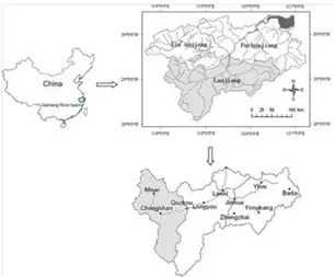
The study area is located in the upper reaches of the Qiantang river basin, located in the Zhejiang Province in East China. Quzhou, the city wherefore flow forecasts will be derived, is located in the Lanjiang river basin, which is one of the two important sub-basins of the Qiantang river basin (Xu et al., 2013). The basin Lanjiang is in the southern region of the Qiantang river basin. Quzhou is downstream of a sub-basin of the Lanjiang river basin called the Quzhou river basin (Tian et al., 2014). This basin is therefore relevant in this study (see Figure 1). The Quzhou river basin has a catchment area of 5,290 km2 and is dominated by mountains and hills. The climate in the basin is semi-humid with an annual mean precipitation and temperature of 1500 mm and 15-18 °C respectively. Maximum temperature is about 40 °C. Characteristic for the climate are the hot and rainy summers and cold and dry winters. More than 50 % of the annual precipitation occurs from May to July.

There are three meteorological stations in the study area and one discharge station (Quzhou). The station in Quzhou observes the discharge, precipitation and evaporation. The other two stations in Misai and Changshan only observe precipitation.

16

2.2.

Observed data

Observed precipitation is used for the validation of the GR4J model, for the bias correction of the raw TIGGE ensemble precipitation data and for the perfect forecast simulations for the evaluation of the flood forecasts. Observed discharge is used for the validation of the GR4J model; for the evaluation of the ensemble forecasts and for the hydrological updating procedure used in this study to update the model states every time step during the forecast period. Temperature data is used to calculate the climatological potential evapotranspiration. The climatological value for the potential evapotranspiration will be used, which is a seasonally variable evapotranspiration, because the TIGGE archive does not have forecasts of evapotranspiration. In addition, previous studies have shown that there were no systematic improvements in the rainfall-runoff model efficiencies when using temporally varying evapotranspiration for the GR4J model and the other GR models (Oudin et al., 2005).

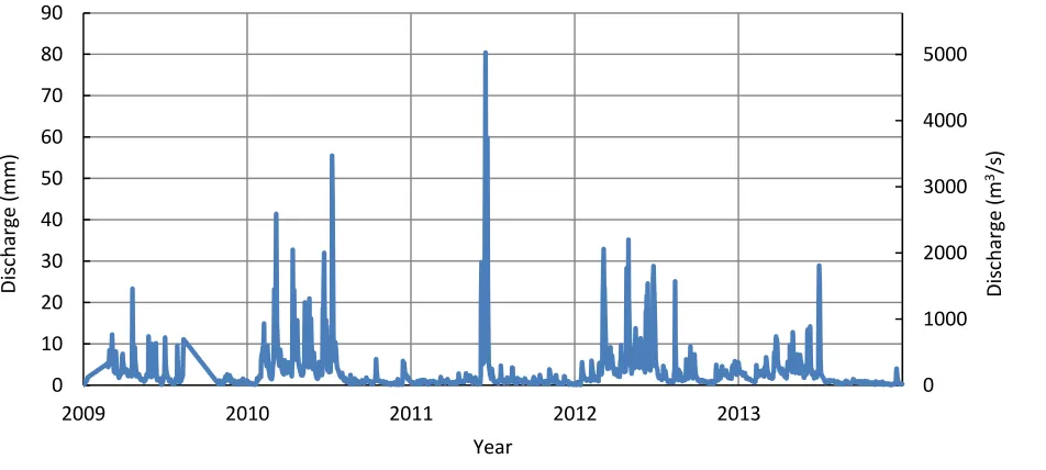
Observed precipitation data come from three meteorological stations in the Quzhou river basin: Quzhou, Misai and Changshan. Observed discharge data comes from the Quzhou meteorological station (see section 2.1). The data are available for the period 01/01/2009-31/12/2013 and are issued at the time step 00:00 UTC. Figure 2 show the timeseries of the areally averaged observed daily precipitation and Figure 3 the timeseries of the observed daily discharge. Figure 3 shows that there are two periods with errors. Missing values of the observed daily discharge are interpolated and are therefore not similar to the historic discharges (see Figure 4). These periods with interpolated values will therefore not be used in this study.

Figure 2 Pluviograph of observed daily areally averaged precipitation for the period 2009-2013. Data is retrieved from the meteorological stations Quzhou, Misai and Changshan.

0 20 40 60 80 100 120

2009 2010 2011 2012 2013

Prec

ip

ita

tio

n

(m

m

/d

)

17

Figure 3 Hydrograph of the observed daily discharge for the period 2009-2014. Data is retrieved from the Quzhou meteorological station.

Figure 4 Errors in the timeserie of the observed daily discharge.

2.3.

TIGGE ensemble precipitation forecast data

The TIGGE network consists of several NWP centres which generate ensemble forecasts and covers large parts of the globe and is detailed enough to use for flood forecasting. Therefore, the TIGGE network has great potential for global scale forecasting and has been used in many hydrometeorological forecasting studies (Ye et al., 2014). TIGGE is a component of THORPEX. THORPEX is the World Weather Research Programme project with the aim to accelerate improvements in the accuracy of 1-day to 2-week high-impact weather forecasts (Bougeault et al., 2010). TIGGE is a key component to achieve this aim and was initiated in 2005. Several studies showed already that the TIGGE database can produce an improved early flood warning of up to 10 days ahead (He et al., 2010). TIGGE develops a deeper understanding of the contribution of observation, initial and model uncertainties to forecast error and investigates new methods of combining ensembles from different sources to correct systematic errors (Bougeault et al., 2010).

0 1000 2000 3000 4000 5000

0 10 20 30 40 50 60 70 80 90

2009 2010 2011 2012 2013

Dis

ch

ar

ge

(m

3/s

)

Dis

ch

ar

ge

(mm

)

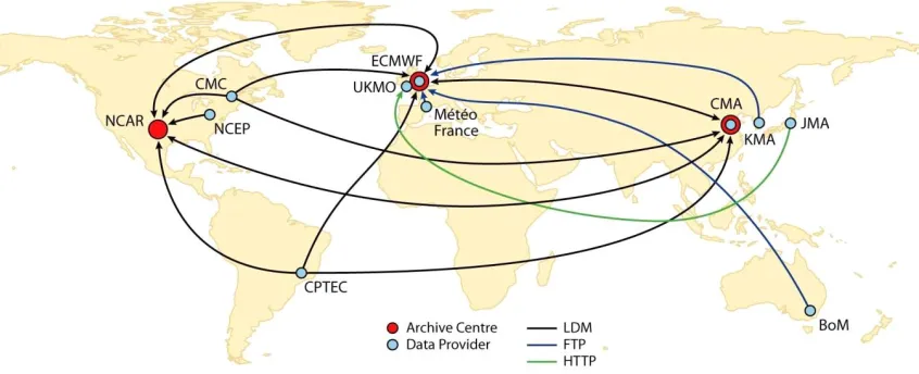
18 Ten centres supply daily forecasts to the TIGGE archive (Park et al., 2008). Nine of these centres are running a medium-range global ensemble prediction system: European Centre for Medium-Range Weather Forecasts (ECMWF); US National Centers for Environmental Prediction (NCEP); Meteorological Service of Canada (MSC); the Australian Bureau of Meteorology (BoM); the Chinese Meteorological Administration (CMA); the Brazilian Centre for Weather Prediction and Climate Studies (Centro de Previsao de Tempo e Estudos Climáticos, CPTEC); the Japanese Meteorological Administration (JMA); the Korean Meteorological Administration (KMA); and the UK Met Office (UKMO) . Météo-France has a short forecast range. In Park et al. (2008) a medium-range global ensemble system is formulated as an ensemble system designed to provide probabilistic forecasts for at least up to 7 days and for the whole globe.

Ensemble prediction systems are designed to represent the effect on weather forecasts of observation uncertainties, imperfect boundary conditions and data assimilation assumptions and model uncertainties (Park et al., 2008). Model uncertainties may occur due to a lack of resolution, simplified parameterization of physical processes and the effect of unresolved processes. Data-assimilation assumptions may occur due to the data-assimilation methods and underlying statistical assumptions. When a grand ensemble of EPS from different weather centres combined is used also other sources of uncertainties, including numerical implementations and/or data assimilation, can be assessed (He et al., 2010). The aggregation of various models that produce EPS from different weather centres also results in a better retaining of and accounting for the probabilistic nature of the ensemble precipitation forecasts (Bao et al., 2011).

The TIGGE ensemble prediction systems are based on several time integrations of a numerical weather prediction model, with the control forecast starting from a 'central' analysis, this is the unperturbed analysis generated by a data-assimilation procedure, and the other perturbed forecasts starting from perturbed initial conditions defined to simulate the effect of initial condition uncertainties (Park et al., 2008).

19

Figure 5 The TIGGE network with its data providers and archive centres (Orientplus, 2015).

2.4.

Content and format of the TIGGE archive

Bougeault et al. (2010) described the content and format of the archive. Fields in the TIGGE dataset are described by the following attributes: analysis date, analysis time, forecast time step, origin centre, ensemble member number, level, and parameter. The parameter in the TIGGE dataset refers to the physical quantity represented by the field and is in this research precipitation only, because for the other input parameter, evapotranspiration, the daily climatological value is used.

Data providers preserve their original model grids and resolutions whenever possible to guarantee the best precision (Bougeault et al., 2010). Therefore they can choose their own horizontal grid to supply their data on, which will be as close as possible to the computational grid of their model. The data are stored in the database in their original state. However, users usually want data interpolated on common regular grids of their own choice. Therefore, the archive centres offer an interpolation service. This interpolation service allows users to interpolate data to a single point or to a regular, limited-area, or global latitude-longitude grid specified to their own choice.

Data used from the TIGGE archive

20 data period does not cover the whole data period of available observed data. This is because there are missing data in the TIGGE archive of the CMA model from 30/10/2013 till 14/11/2013. Also noteworthy is that the retrieved data from the TIGGE archive starts at 17/12/08, because for bias correction of the data a moving window of 31 days will be used (15 days before and 15 days after the forecast issue date). The resulting validation period of the TIGGE data will be from 01/01/2009 to 14/10/2013. The TIGGE data are retrieved for the time step 00:00 UTC to get along with the other observed data which is also issued on 00:00 UTC. There is one missing forecast in the NCEP forecast data in the data period of retrieved TIGGE data. Su et al. (2014) had the same problem for the NCEP forecast dataset. They considered that replacing this small fraction of data will not influence the final results. The missing NCEP forecast data are therefore replaced with the interpolated value of precipitation values of the day before and after this missing day.

The data retrieved from TIGGE is the accumulated total precipitation. The data are processed to 24 hour accumulated precipitation values by the subtraction of the accumulated total precipitation of the lead time -1 day. However, after this process there are some negative values. Small negative values (-1 - 0 mm/d) are caused by the scaling of values during Gridded Binary (GRIB) packing or interpolation errors (ECMWF, 2013). All negative values of 24 hour precipitation forecasts are set to zero which was also done by Su et al. (2014).

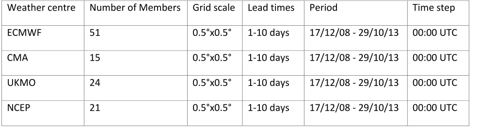
Table 1 Weather centres and their properties used in this study (ECMWF, 2015)

Weather centre Number of Members Grid scale Lead times Period Time step

ECMWF 51 0.5°x0.5° 1-10 days 17/12/08 - 29/10/13 00:00 UTC

CMA 15 0.5°x0.5° 1-10 days 17/12/08 - 29/10/13 00:00 UTC

UKMO 24 0.5°x0.5° 1-10 days 17/12/08 - 29/10/13 00:00 UTC

NCEP 21 0.5°x0.5° 1-10 days 17/12/08 - 29/10/13 00:00 UTC

2.5.

GR4J model

2.5.1. Model description

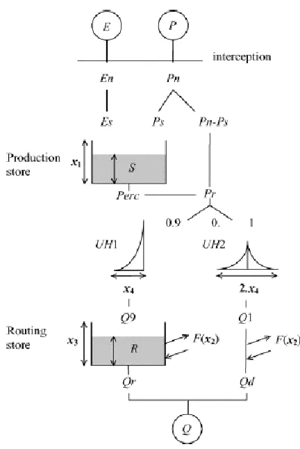
21 unit hydrographs together with a calculated groundwater exchange F into a catchment outflow. The GR4J model consists of four parameters that have to be optimised for the catchment by the use of observed discharge:

x1: maximum capacity of the production store (mm)

x2: groundwater exchange coefficient (mm)

x3: one day ahead maximum capacity of the routing store (mm)

x4: time base of unit hydrograph UH1 (days)

All these four parameters are real numbers. x1 and x3 are positive, x2 can be either zero, negative or

positive and x4 is greater than 0.5. The GR4J model runs at daily time steps.

Figure 6 Model structure of the GR4J rainfall-runoff model (Perrin et al., 2003)

2.5.2. Calibration and validation of the GR4J model

22 parameter set with the maximum NS value. Also the Relative Volume Error (RVE) was calculated for the optimum parameter set.

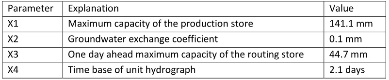
The maximum NS value for the Quzhou River Basin in the calibration period was 0.93 and the corresponding RVE was -1.1. The obtained optimum parameter set for the Quzhou river basin is presented in table 2.

Table 2 Optimum parameter set for the Quzhou river basin (Tian et al., 2014)

Parameter Explanation Value

X1 Maximum capacity of the production store 141.1 mm

X2 Groundwater exchange coefficient 0.1 mm

X3 One day ahead maximum capacity of the routing store 44.7 mm

X4 Time base of unit hydrograph 2.1 days

23

3.

Methods

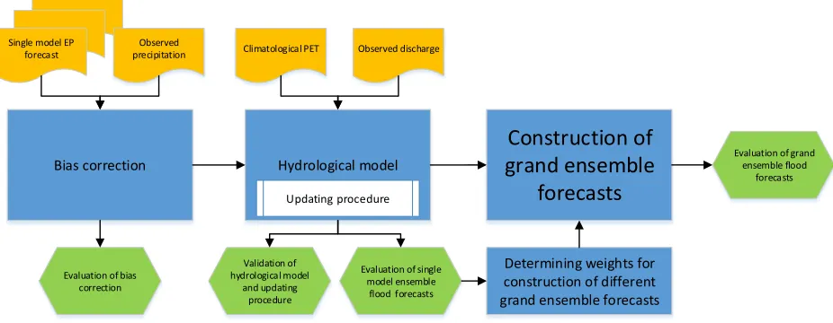
This chapter describes the methods used in this study to develop the ensemble flood forecasting system and the grand ensembles. Also the evaluation methods are described. In section 3.1 the bias correction approach is described. Section 3.2 describes the updating procedure used in this study. Section 3.3 describes the evaluation methods to evaluate the ensemble forecasts. The last section describes the combination method of the EPSs to construct a grand ensemble forecast. Figure 7 shows a flow chart of the forecasting system.

Bias correction Hydrological model

Evaluation of bias correction

Construction of

grand ensemble

forecasts

Evaluation of single model ensemble

flood forecasts

Evaluation of grand ensemble flood

forecasts

Updating procedure

Validation of hydrological model

and updating procedure

Determining weights for construction of different grand ensemble forecasts

Single model EP forecast

Observed

precipitation Climatological PET Observed discharge

Figure 7 Flow chart of the methods used in this study (Blue objects form the Ensemble forecast system; Orange objects are the input data of the Ensemble forecast system; Green objects are various evaluations steps in this study).

3.1.

Bias correction Quantile mapping method

In general the raw ensemble forecasts from NWP models are biased in the mean and spread (Wu et al., 2011). Bias is the systematic difference between the forecast and its verification which is often an observation. Even if the forecasts are not biased at the model grid scale, they may be biased at the catchment scale, due to heterogeneity in the forecasted variable within the model grids. This is depending on the size of the basin. Correcting such biases is normally referred to as post-processing or statistical calibration. There are four reasons why EPSs in flood forecasting systems usually require some kind of meteorological post-processing (Tao et al., 2014):

1. The accuracy of the raw ensemble meteorological forecasts evaluated at grid size is still limited and not suitable for direct hydrological modelling to forecast floods, even though the ensemble meteorological forecasts have been improved significantly.

2. The spread of the raw meteorological ensembles may be unreliable / underdispersed.

24 4. The temporal resolution of meteorological ensemble forecasts is not equivalent to those

required for generating hydrological forecasts.

Bias-correction for precipitation ensemble forecasts has proven to be very challenging because of the large space-time variability of precipitation (Wu et al., 2011). Wu et al. (2011), therefore expect that significant additional efforts will be needed to produce operational ensemble forecasts that are good enough for hydrological applications, especially for large precipitation amounts and small catchments. Statistical methods are often used for post-processing and downscaling raw meteorological ensemble forecasts. Statistical downscaling is often performed to correct for point 3 and 4 in the numeration above. However, since the TIGGE archive centres offer an interpolation service, downscaling of the raw meteorological ensemble forecasts is done with this service. In 2.4 was described that the data is downloaded at a resolution of 0.5° x 0.5° which is comparable to the observation and the GR4J model used. Therefore the focus in this section is on the bias correction method to correct for point 1 and 2. Systematic bias is unavoidably present in the precipitation forecasts, and is usually a function of spatial location and forecast lead time (Voisin et al., 2010). For stream flow forecasting a preferred approach of bias correction is to use a bias correction transformation to correct all model-simulated ensemble time series (Hashino et al., 2007), because bias-corrected ensemble time series can be used in water resources applications. One of these bias correction methods is the quantile mapping method.

The quantile mapping method uses the cumulative distribution functions (CDF) for observed and simulated values for each lead time to remove the biases. The quantile mapping method tends to improve the skill score and tends to lead to high sharpness (the tendency of the forecast to predict extreme values (WMO, 2015)) and discrimination (the ability to discriminated among observations, meaning that forecasts have higher prediction frequencies for event occurrences and lower for nonoccurrences (WMO, 2015)) (Hashino et al., 2007) . Therefore this method is used in this study. Forecasts have discrimination when the forecasts issued for different outcomes (event occurrences or nonoccurrences) are different. Hence, for forecasts to have good discrimination, they must both be sharp and have high potential skill

The bias correction of quantile-based mapping is achieved by replacing the forecasted value with observed values with the same percentiles (nonexceedance probabilities) (Voisin et al., 2010). Bias correction is done for each day and each lead time in the set of 10-day forecasts in the period 2009-2013. The corresponding method is as follows:

1. Derivation of the forecast daily cumulative distribution function (CDF)

25 forecasts only 15 members x 31 days x 4 or 5 years = 1860 or 2325 values have to be ranked. The CDF of UKMO consists of 24 members x 31 days x 4 or 5 years = 2976 or 3720 values and of NCEP 21 members x 31 days x 4 or 5 years = 2604 or 3255 values.

2. Derivation of the observed daily CDF

The Jan 2009 - Sept 2013 daily precipitation datasets from the different weather stations in the Quzhou river basin were interpolated with the Thiessen Polygon method to daily areally averages. The CDF of the observed daily areally average precipitation is also derived for a 31 day moving window. Using the 31 day moving window, in between 31 days x 4 and 5 years = 124 and 155 values had to be ranked in each CDF; depending on how many times the issued date is in the dataset. The daily CDFs were derived for each day, so 366 CDFs were derived.

3. Quantile mapping

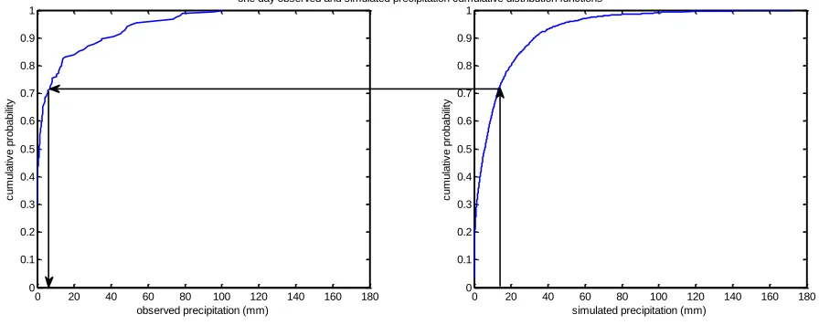
The quantile mapping approach is applied to each daily ensemble forecast set in the Jan 2009 - Oct 2013 period. Each ensemble member and each lead time of the different EPSs is corrected with the quantile mapping approach independently so that different biases at different lead times can be corrected and that the forecast can be corrected in the spread. The quantile (Qn) of the daily precipitation forecast member is estimated in the corresponding forecast CDF (appropriate day, centre of the 31 days moving window, and lead time. This estimated quantile is substituted for the observed value with the same quantile in the corresponding daily CDF (CDF for that day and lead time) (see Figure 8). The corresponding definition of the quantile mapping method is as follows:

Where is the bias-corrected forecast value, is the forecast value, is the CDF of the observed climatology, is the forecasted CDF, and Qn is the quantile of the forecast value in the forecast CDF.

Figure 8 Quantile mapping approach with the daily observed and simulated precipitation cumulative distribution functions

0 20 40 60 80 100 120 140 160 180 0

0.1 0.2 0.3 0.4 0.5 0.6 0.7 0.8 0.9 1

observed precipitation (mm)

c

u

m

u

la

ti

v

e

p

ro

b

a

b

ili

ty

0 20 40 60 80 100 120 140 160 180 0

0.1 0.2 0.3 0.4 0.5 0.6 0.7 0.8 0.9 1

simulated precipitation (mm)

c

u

m

u

la

ti

v

e

p

ro

b

a

b

ili

ty

26

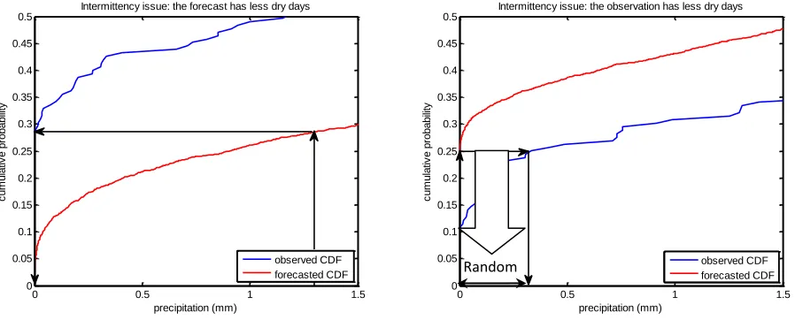
4. Daily precipitation intermittency correction

The quantile mapping method is limited when dealing with intermittency. Intermittency is defined as the difference in the dry day frequency of the raw model output and the observations. The precipitation intermittency issue can occur in two ways. First there is the case that the forecasts have less dry days than the observations and second the case that the forecasts have more dry days than the observations. In the first case the intermittency is automatically corrected by the quantile mapping bias correction method. The quantiles of the forecast distribution below the no-precipitation threshold in the CDF of the observations are defined as dry (Figure 9a). However, for the second case, when the forecasts have more dry days than the observation the intermittency is not automatically corrected by the quantile mapping bias correction method. Using the quantile mapping method for bias correction in this case leads to a strong positive bias after the correction (Figure 9b). Therefore, an intermittency correction approach is implemented for the bias correction of the precipitation forecasts. In this intermittency correction approach quantiles are randomly selected between zero and the corresponding quantile of the no-precipitation threshold from the forecasted CDF. The corresponding observation quantile of this randomly selected quantile may or may not be associated with precipitation. This approach can be presented as follows:

Where Qnobs and Qnfcst are respectively the largest observed and forecast quantiles associated with a

zero precipitation value.

Figure 9 Intermittency issues: the forecast has less dry days then the observation (left); the observation has less dry days then the forecast (right)

0 0.5 1 1.5

0 0.05 0.1 0.15 0.2 0.25 0.3 0.35 0.4 0.45 0.5 precipitation (mm) c u m u la ti v e p ro b a b ili ty

Intermittency issue: the observation has less dry days

observed CDF forecasted CDF

0 0.5 1 1.5

0 0.05 0.1 0.15 0.2 0.25 0.3 0.35 0.4 0.45 0.5 precipitation (mm) c u m u la ti v e p ro b a b ili ty

Intermittency issue: the forecast has less dry days

observed CDF

27

3.2.

Hydrological updating

3.2.1. Introduction

As described before there are many sources of errors, when forecasting runoff. In ensemble flood forecasting forecasted precipitation input data are used in hydrological models to extend lead times. This generates a major uncertainty for the hydrological forecasting system (Kahl & Nachtnebel, 2008). As a result the simulated and forecasted hydrographs will never fit perfectly to the measurements. To compensate the input and model uncertainties partially, techniques have been developed to minimize errors in simulation of the recent history and improve the forecast. Errors in the recent past can influence the forecast negatively. Therefore updating procedures are developed to update model input, state/storages and output so that the current situation in the river basin is better represented (Wöhling et al., 2006).

Popular updating procedures are Auto Regression models and Kalman filtering, however these procedures are not suitable for short forecast periods and steep flood hydrograph characteristics which are typical for small, quickly reacting mountainous catchments such as the Quzhou catchment area (Wöhling et al., 2006). For this kind of catchments it is the primary goal to extend the forecast lead time. Moreover, classical updating procedures, such as Auto Regression models, focus on the river flow itself which leads to a significant loss of forecast lead time in small, quick reacting catchments. Also more complicated procedures, such as Kalman filtering, are mathematically too complex to be easily accommodated in highly non-linear models. Therefore a simple effective updating procedure developed by Demirel et al. (2013) for the GR4J model is used to minimize errors in the initial state.

3.2.2. Updating procedure developed by Demirel et al. (2013)

The updating procedure developed by Demirel et al. (2013) is a model storage update procedure based on the observed discharge on the forecast issue day. This is an important step for medium-range flow forecasts since the model initial state determines the model outputs. The routing storage variable in the GR4J model is updated during the flow forecasts with using this approach. In GR4J the simulated runoff Q is calculated with the fast runoff component Qr and slow runoff component Qd with the following formula:

The fast runoff component and slow runoff component in the GR4J model can be estimated with the use of the empirical relations between the simulated discharge and the fast runoff to divide the observed discharge between the fast and slow runoff components. With this empirical relation a fraction k of the slow runoff component compared to the simulated discharge can be calculated:

28

In the GR4J model the outflow Qr is calculated as:

Since Qr and Qd are updated with the equations above, the routing storage (R) will be updated for a given value of the X3 parameter by inverting the latter equation. This updated routing storage is used for the calculation of the forecast of the next day.

3.2.3. Implementation in the ensemble flow forecasting system

The updating procedure in this study provides initial model storages for the forecast issue day based on the observation and the simulation of the day before the forecast issue date. This is the approach for a lead time of 1 day. If this approach would be used for longer lead times the model states would be updated with the observation value of lead time days before the forecast issue date. This approach would result in a fast decrease in the performance of the model, since the autocorrelation is decreasing fast with lead time in a small mountainous quick reacting catchment. Therefore the initial states are not updated with the approach for lead times longer than 1 day. Instead, the initial states calculated with the GR4J model of the previous lead time are used (see Figure 10).

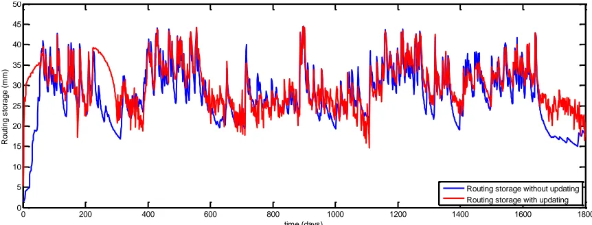
3.2.4. Check whether the hydrological updating procedure is realistic

To ensure the hydrological updating procedure is realistic, the routing storages with and without the hydrological updating procedure are calculated over the validation period. With this comparison it becomes clear whether the use of the hydrological updating procedure results in tuning (small difference) or curve fitting (big difference) of the new simulated discharges. If the routing storages change in order of magnitude with the implementation of hydrological updating, the predictive power of the GR4J model is weakened.

29

Ensemble Discharge forecasts Q1 GR4J model t=1

Input: Ensemble Forecasts Pt=1

Climatological PET

Observed discharge

Initial model state

Updating procedure

GR4J model t=2

Initial model state for next lead time

GR4J model t=10 Initial model state for next lead time

Input: Ensemble Forecasts Pt=2

Climatological PET

Input: Ensemble Forecasts Pt=10

Climatological PET

Initial model state for next lead time Input:

Ensemble Forecasts Pt=t Climatological PET

GR4J model lead time t=3 - 10

Ensemble Discharge forecasts Q2

Ensemble Discharge forecasts Qt=t

Ensemble Discharge forecasts Q10

Figure 10 Ensemble flow forecast system with updating system. Blue objects are the processes, orange are the input data, green are the initial model states (routing storage) and pink are the output ensemble discharge forecasts.

Figure 11 Routing storage (mm) with and without updating for the period 2009-2013 for lead time 1.

0 200 400 600 800 1000 1200 1400 1600 1800

0 5 10 15 20 25 30 35 40 45 50

time (days)

R

o

u

ti

n

g

s

to

ra

g

e

(m

m

)

Hydrological updating

30

3.3.

Evaluation methods

Evaluation methods monitor and compare the quality of forecasts and identify the strengths and weaknesses of the forecast system (Tödter & Ahrens, 2012). Evaluation possibly allows a future improvement.

Three properties of an accurate probability forecast system are defined in WMO (2015):

 Reliability: the agreement between forecast probability and mean observed frequency of an event. The closer the mean observed frequency matches the forecasted probability, the more reliable the forecasts are.

 Sharpness: the tendency to forecast probabilities of an event occurring near 0 or 1 instead of values clustering around the mean. So, the tendency of the forecast to predict extreme values.

 Resolution: the ability of the forecast to resolve the set of sample events into subsets with characteristically different outcomes. It measures how much the conditional probabilities given the different forecasts differ from the climatic average. Even if the forecasts are wrong, the forecast system has resolution if it can successfully separate one type of outcome from another. To assess these properties, and evaluate probabilistic forecasts, several statistical evaluation measures have been proposed in the literature such as the Brier score, the ranked probability score, the continuous rank probability score, the reliability diagram and the rank histogram (Cloke & Pappenberger, 2009). The ranked probability score and the continuous ranked probability score would enable to assess the overall quality of the ensemble, or the quality on a certain range of the forecast. The BS on the other hand permits to focus on specific warnings and thresholds meaningful for studies to flood forecasts. The BS is chosen for this study as it permits to look at specific thresholds and also two out of the three properties defined above that describe an accurate forecast can be calculated, namely reliability and resolution. The other property, sharpness, can be shown by a reliability diagram with a corresponding sharpness diagram and will therefore also be used in this study. Next to these two evaluation methods the continuous ranked probability score and the root mean square error will be used for the combination of the different TIGGE ensemble forecast models and for the evaluation of the overall performance of the forecasts.

3.3.1. Thresholds

The forecasts will be evaluated at certain thresholds derived from the observed precipitation and discharge. Since this study focus on high flow forecasts the thresholds chosen in this study are quantile 75%, 85% and 95% with an exceedance of 25%, 15% and 5% respectively. Both precipitation forecasts and discharge forecasts are evaluated, so P75, P85 and P95 as well as Q75, Q85 and Q95 of the observed data will be used. Table 3 show the threshold values for the precipitation and discharge evaluation.

31

Table 3 Precipitation and discharge thresholds used in this study

Thresholds 75 % 85 % 95 %

Precipitation (mm) 5.31 12.31 27.75

Discharge (mm) 3.77 5.52 11.68

3.3.2. Evaluation of the forecast against reference flow

As described before hydrological forecasts used in this study contain both errors from the meteorological forecasts and the hydrological model. When evaluating these hydrological forecasts against observed discharge a third error component is present: the discharge observation measurement error (Renner et al. 2009). However, in the hydrological model used here the updating procedure also uses discharge observations to update the initial state of the routing storage of GR4J. So the discharge observation measurement error is also present in the hydrological forecasts. To give better interpretation of the forecast performance and come to better conclusions it is useful to know where the largest errors in the forecasting system are coming from. To see which errors have the largest influence some of the errors have to be removed from a reference flow. This can be done by using perfect flow forecasts as reference flows. In this case the hydrological model error component and discharge observations measurement error component are removed from the evaluation with the hydrological forecast, because both forecasts contain these two errors. With the elimination of two errors it is still not possible to know if the meteorological error contributes more to the hydrological error than the hydrological model error. However, if it is assumed that observation errors can be neglected, evaluation of the forecasts against perfect flow forecasts contain error components from the meteorological forecasts, while evaluation against observed discharge contain both error components from the meteorological forecasts and the hydrological model. For the general scores of the deterministic evaluation measure (RMSE) and probabilistic evaluation measure (CRPS) this comparison of evaluation against observation and perfect flow forecast will be made. It is not possible to do a simpler comparison with the evaluation scores of flow forecasts and meteorological precipitation forecasts, because the evaluation scores of RMSE and CRPS depend on the magnitude of the investigated parameter (discharge and precipitation respectively).

3.3.3. Deterministic evaluation

The root mean square error (RMSE) is common used in forecast evaluation. The RMSE is not a probabilistic evaluation measure but a deterministic evaluation measure (WMO, 2015). So when calculating the RMSE for a probabilistic forecast like the TIGGE ensemble forecasts first the ensemble mean have to be calculated. The RMSE is defined as:

32 The RMSE is used in this study as extra evaluation of the forecasts next to the probabilistic evaluation and as a measure where weights for Grand Ensembles will be based on. Since other weighting methods are based on the CRPS it is interesting to see if the RMSE as well as the CRPS will improve when using a Grand Ensemble based on the RMSE or CRPS of single models.

3.3.4. Probabilistic evaluation

3.3.4.1. Continuous Ranked Probability Score (CRPS)

The CRPS is also often used as an evaluation method for probabilistic forecasts. The CRPS is an evaluation tool that evaluates the accuracy of a probabilistic forecast distribution by comparing the distribution of an ensemble of forecasts to the observed value (Liu & Xie, 2014). The CRPS has some interesting properties. First, it is sensitive to the entire permissible range of the parameter of interest, discharge in this case. Second, its definition does not require the introduction of a number of predefined classes on which results may depend as is the case with the ranked probability score. The CRPS takes instead of the ranked probability score the limit of an infinite number of classes, each with zero width (Hersbach, 2000). This avoids loss of information and sensitivity of the score to the number and choice of the thresholds values (Tödter & Ahrens, 2012). Last, the CRPS is equal to the mean absolute error for a deterministic forecast; it therefore has a clear interpretation. The CRPS is an evaluation method that is sensitive to the overall (with respect to a certain variable) performance of a forecast system. The CRPS of a probability forecast is defined as:

where n is the number of forecasts, F(x) is the forecast cumulative distribution function (CDF), O(x) is the observed CDF. H(x-x0) is the Heaviside function that jumps from 0 to 1 at the observed value, if x < xo,i,

33

Figure 12 Example of a cumulative distribution for an ensemble {x1, ... , x5} of five members (blue line) and for the verifying analysis of the observation xo (red line), the CRPS is represented by the shaded area. (Hersbach, 2000)

The calculation of the CRPS will be done for the cases where the observation is above the Q75 value, for the evaluation of the forecasts and the calculation of the weights for the combination of the forecasts.

3.3.4.2 Continuous Ranked Probability Skill Score (CRPSS)

The CRPSS is a normalized form of the CRPS. The CRPS is normalized by a reference which is usually the climatology or persistence of a study area. The Continuous Ranked Probability Skill Score (CRPSS) is used to evaluate the quantitative skills of the ESP to study the added value of the probabilistic forecasts. CRPSS is defined as (e.g. Hersbach, 2000):

CRPSS measures the improvement of an ensemble forecasting system over the reference forecast. The reference forecast is an alternative forecast and is in this study compared to the hydrological forecast. The value of CRPSS ranges from -∞ to 1 (Alfieri et al., 2014). CRPSS gives a score of 1 when the forecast has perfect skill, while negative values indicate worse performance than its reference forecast. So EPSs are only valuable when CRPSS > 0. In that case the forecast is performing better than the reference forecast.

34 et al. (2013) and Pappenberger et al. (2015) both advise to use a reference forecast of an ensemble of hydrological forecasts calculated by the hydrological model using historical meteorological observations at the same calendar day as input to the model, because this leads to the lowest CRPS values of the reference forecast. Thus the reference forecast has the same number of ensembles as the number of years in the reference period. An ensemble of precipitation and potential evapotranspiration is used here to run the hydrological model with updating and compute the reference forecast and the corresponding CRPSreference for the same validation period as for the forecast from 1 January 2009 to 15

October 2013. The reference forecast consists of 10 ensemble members, because the period of reference is from 1981 to 1990.

The CRPSS will be used in this study to evaluate the added value of the forecasts over the reference forecast.

3.3.4.3 Brier Score

The Brier score is a relatively simple and often used evaluation method for probabilistic forecasts and is one of the oldest evaluation tools in use (Hersbach, 2000). The Brier score takes instead of the CRPS with an infinite number of classes, each with zero width, only two classes into account. The Brier score is essentially the mean squared error of the probabilistic forecast and evaluates the accuracy of the probabilistic forecast at a chosen threshold (Wilks, 2006). Usually, Brier scores are evaluated for different threshold levels. The Brier score has the attractive property that it can be decomposed into a reliability, a resolution, and an uncertainty part (Tödter & Ahrens, 2012). The reliability is the mean conditional bias and quantifies the calibration of the forecast system. The resolution measures the average distance of all climatological probability of observed occurrence to the unconditional probability of occurrence. Here large differences are preferable. The last term, uncertainty, measures the variance of the observations. It is only dependent on observed data and therefore for each lead time the same. Brier scores thus should not be compared on different samples. With the decomposition of the Brier score you can obtain a detailed insight into the performance of the forecast system with respect to the event under consideration (Hersbach, 2000). The Brier score has the advantage that it can be applied to both deterministic and probabilistic forecasts, without the need to transform the ensemble forecast into a deterministic one (e.g. by considering the median only) (Addor et al., 2011).The Brier score is defined as:

where the index k denotes a numbering of n forecasts, fk is the forecasting probability that was forecasted and ok is the actual outcome of the event at instance k (ok=1 if the event occurs, otherwise

ok=0) (Wilks, 2006).

When decomposed into the three components: reliability, resolution and uncertainty the Brier score is defined as:

35 where is the observed climatological base rate for the event to occur, is the observed frequency of occurrence of events at instance k, given the forecasting probability .

The Brier score is negatively oriented, so it assigns better forecasts lower scores. The score can only take on values in the range 0 ≤ BS ≤ 1, since individual forecasts and observations are both bounded by zero and one (Wilks, 2006).

3.3.4.4. Reliability diagram

The reliability diagram and sharpness diagram are commonly used for the evaluation of probabilistic forecasts. They measure reliability, resolution and sharpness (three important attributes of a good probability forecast system).

Reliability diagram

The reliability diagram consists of a plot of the observed relative frequency against the predicted probability of the forecasts. In other words, it measures how closely the forecast probability of an event corresponds to the actual chance of observing the event. The reliability diagram provides a quick visual inter-comparison between for example different thresholds or different forecasts (Bröcker & Smith, 2007) and can evaluate the reliability and the resolution of a forecast.

In the evaluation of the reliability diagram the observed relative frequency of exceeding a threshold is compared with the predicted probability of exceeding a threshold over a set of probability bins. The diagonal line indicates perfect reliability (in this case the average observed frequency is equal to the predicted probability for each category). The horizontal deviation of a forecast from this line indicates the "conditional bias". If the curve of the forecast lies below the diagonal, the probabilities are too high and this indicates overforecasting; if the curve of the forecast lies above the diagonal this indicates underforecasting and the probabilities are too low (Figure 13 left). The vertical deviation from the horizontal climatology line in the reliability diagram indicates the resolution of the forecast (Figure 13 right). So the flatter the curve in the reliability diagram the less resolution a forecast has.

36

Figure 13: Example of a reliability diagram with the deviation from the reliability line to measure the reliability (left) and the deviation from the climatology line to measure the resolution (right)

Sharpness diagram

A reliability diagram is often seen in combination with a sharpness diagram of the forecast, to which it is closely connected. The sharpness diagram shows the relative frequency of the forecasts exceeding a certain threshold over the reference period in each probability bin of the set of probability classes of the reliability diagram (0%-20%, 20%-40%, 40%-60%, 60%-80% and 80%-100%). As defined before, forecast systems that are able to predict events with probabilities different from the observed event frequency are said to have 'sharpness'. Forecast systems with little sharpness would have a frequency peak near the climatological frequency and therefore indicate that the most of the forecasts predict the event with a probability near the climatological frequency. These forecast systems therefore offer little value for planning purposes over simple use of the observed climatology.

The reliability diagram and sharpness diagram are applied in this study next to the other evaluation measures to compare the forecasts qualitatively and to give insight in the sharpness of the forecasts, as sharpness is described as one of the three important attributes of a good probability forecast system.

3.4.

Combination methods for grand ensembles

37 being much smaller in size. This implies that the combination is more important than the increase in ensemble size.

Even though a multi-model ensemble combines the strengths from different models, some model might perform better than others at different times and for different catchments (Johnson & Swinbank, 2009). Therefore further improvements of the multi-model ensemble might be realized by giving the models different weights. In the introduction is described that previous research has shown that model-dependent weights can give improvement, but that caution should be taken in how they are calculated and used (e.g. Raftery et al., 2005; Stefanova & Krishnamurti, 2002). For example, Raftery et al. (2005) used Bayesian Model Averaging (BMA) model-dependent weights to construct their grand ensemble and concluded that they created a better deterministic forecast. Section 3.4.1 describes the combination procedure and in section 3.4.2 the weighting methods used in this study are described and supported.

3.4.1. Combination procedure

The combination procedure can be described with the use of the law of total probability (Raftery et al., 2005). Following Raftery et al. (2005) the multi-model probability density function (PDF) of the variable x is then given by an average of the PDFs from the single-models:

where is the pdf based on model and is the probability of being the best model and can be viewed as model-dependent weights . Thus, , where and

.

In more detail this combination procedure can be described as follows. The multimodel ensemble is given by the union of the ensemble members from the single model ensembles for each time step and lead time. Johnson and Swinbank (2009) derived mean probabilities and ensemble mean from the multi-model ensemble combination procedure of Raftery et al. (2005) which can be used for the calculation of the Brier score, CRPS, RMSE and reliability diagrams.

The multi-model ensemble mean probability derived is:

where M is the number of models, is the weight for single model k and is the single model probability given by the following formula:

38 The formula for the single model probability is used for the calculation of the Brier score, CRPS and the reliability score for the single model performance. While, the formula of the multi-model ensemble probability is used for the calculation of the Brier score, CRPS and the reliability diagram for the different multi-model combinations.

The multi-model ensemble mean is given by:

wherein is the single-model mean which is given by the following formula:

The formula for the single-model means is used for the calculation of the RMSE of the single model performance. The formula of the multi-model ensemble mean can be used for the calculation of the RMSE of the different multi-model combinations.

3.4.2. Combinations based on weights

Since the models used in this study have different numbers of ensemble members there are two basic combination methods for the single model forecasts to construct the grand ensemble (see Figure 14). The first alternative is to combine all ensemble members in the grand ensemble in a single distribution where the multi-model mean forecast and the multi-model mean probability is given by the average forecast value and the average ensemble probability of the ensemble members from all models. In this firs alternative the model with more members will get more weight. The second alternative is to combine the models in the grand ensemble. In this case the members of the multi-model are sampled from the individual distributions of the models with the result that the multi-model mean is given by the average of the single model means and the multi-model mean probability is given by the average of the single model mean probability. In this case each single model has the same influence on the multi-model ensemble independent of their ensemble member size.

39 As described before the weights can be viewed as the probability of a particular model being the best model. It is the aim to give more weight to the more skilful models. Johnson and Swinbank (2009) described that there are various methods to define these weights. One method to compute the weights is Bayesian model averaging (BMA), where the weights and variances are computed simultaneously with the use of maximum likelihood estimation and aims to fit the PDFs to the calibration data (Raftery et al., 2005). Another method is the much more simple skill-based method (Johnson & Swinbank, 2009). In this method the weights are dependent on a measure of forecast skill. Despite the methods simplicity, the derived weights are surprisingly similar to those derived from the more complicated multiple-regression and BMA methods, as seen in studies by Raftery et al. (2005) and Johnson (2006). Therefore the skill-based method is used in this study.

Johnson and Swinbank (2009) used the mean squared error to calculate the weights. The mean squared error is a measure of skill based on the mean of the forecast ensembles and does not take the advantages of the ensembles in account. Since CRPS is a measure of skill of the probability of the ensembles this is also an interesting measure of skill to use for the calculation of the weights. Therefore both measures of skill (RMSE and CRPS) are used in this study to calculate the weights and to compare the results of these different weighting methods for the grand ensemble.

In 3.4.1 different formulas are described for the procedure to construct a multi-model ensemble. In the formulas to calculate the ensemble means there is a weighting parameter present. The given weight to each ensemble member of the single models is defined as:

with and depending on the weighting method in this study. is the number of members in model k, skill measurek is the used skill measure to make a

skill based combination. is a normalization factor to ensure that , where M is the number of models used in the combination.

40

Table 4 Grand ensemble set ups used in this study together with their weighting formula used to calculate the weights given to the single model ensembles.

Grand Ensemble abbreviation

Grand ensemble combination method Weight given to single model

ensemble members

GE1 Combination of all members

GE2 Combination of the models

GE3 Combination of the models (weights based on CRPS)

GE4 Combination of the models (weights based on RMSE)

GE5 Combination of the members (weights based on CRPS)

41

4.

Results

The results of this study are divided in five sections. First an example of a simple graphical visualization of the ensemble precipitation forecasts and ensemble discharge forecasts of ECMWF for a typical heavy precipitation period and precipitation peak and a typical high runoff period and runoff peak is given. The second section describes the results of the bias correction of the precipitation forecasts of the EPSs of ECMWF, CMA, UKMO and NCEP. The third section describes results from the hydrological updating procedure used. The fourth section presents the evaluation results of the single model hydrological forecasts. The last section presents the evaluation results of the grand ensemble hydrological forecasts.

4.1.

Pluviographs and hydrographs

Figure 15 shows the observed precipitation and observed discharge from 4-5-2010 to 23-7-2010. It shows that the catchment area is quickly reacting to a rainfall event with a lag time of approximately one day between the rainfall peak (middle of the bar) and the discharge peak.

Figure 15 Observed precipitation and discharge from 4-5-2010 to 23-7-2010 showing the time lag between rainfall and discharge.

Figure 16 and Figure 17 show examples of pluviographs and hydrographs of a typical heavy rainfall and high runoff period and a typical peak precipitation and discharge peak for the observed precipitation and discharge respectively and the precipitation forecast of the ECMWF ensemble and the hydrologic forecast of the ECMWF ensemble respectively. Both figures show that the ensembles sometimes overpredict and sometimes underpredict the precipitation and the discharge. However, the observation almost always falls in the range of the ensembles. The ensemble forecast of the typical peak is an example of a good forecast where the observation falls in the range of the ensembles. The time difference between the precipitation peak and the peak discharge of one day is also visible here when Figure 16 and Figure 17 are compared.

0 10 20 30 40 50 60 70 80 90 100

0 10 20 30 40 50 60 70 80 90 100

Dis

ch

ar

ge

(mm

)

Prec

ip

ita

tio

n

(m

m

/d

ay

)

Date

Observed precipitation and discharge from 4-5-2010 to 23-7-2010