ECE-320: Linear Control Systems Homework 4
Due: Tuesday September 27 at 1PM Midterm Exam October 6!! 1) For the following systems
a) Determine the system type (0, 1, 2, ...)
b) If the system is type 0 assume Gpf =1and determine the position error constant Kp
and the steady state error for a unit step input. Then determine the value of to make this error zero. If the system is type 1, assume
pf
G
1
pf
G = and determine the steady state error for a unit step, the velocity error constant , and the steady state error for a unit ramp. Is there any constant value of that can change the velocity error?
v
K
pf
G
Ans. (steady state errors) 3
2
− , 3
13, 3 5
− , 1
2; (prefilers) 2 5,
13
10, Gpf has no effect
pf
G
+
-5 1
s s
− +
1 3
s+
pf
G
+
-2
s+ 2
5
2 3
s + s+
pf
G
+
-1
s 2
5
2 3
s s
− + +
pf
G
+
-10
s 2
2 2 10
s
s s
2) In this problem we explore a slight change to the standard quadratic optimal controller. We assume we have the following system, with prefilter Gpf , plant G sp( ) and controller
( ) c
G s
pf
G
+
-( )
cG s
G s
p( )
a) Assume the plant is
200 ( )
10 p
G s s
= +
and we want to design a quadratic optimal controller with q=0.001. Show that
0
3.381 0.0169( 10)
( ) ( ) 3.5
11.832 c 8.451 p
s
G s G s G
s s f
+
= =
+ + =
s
=
in order to have a steady state error for a unit step of zero.
Simulate the system with a unit step input. Your results should look like that in Figure 1. Turn in this plot.
b) Assume we utilize the quadratic optimal algorithm as above to determine, G but rather than utilizing a prefilter, we scale the closed loop transfer function so
thatG . Show that we then get
0( )
0(0) 1
0.05916( 10) ( )
c
s G s
s
+
= and Gpf =1
Simulate the system using this controller and prefilter with a unit step input. Your results should look like that in Figure 1.
Note that we are not guaranteed we will be able to get an implementable transfer
function if we scale G0( )s so that G0(0)=1, but if we can, we get a type 1 system and
there is no scaling outside the of the feedback loop (Gpf =1 )! Why do we care? See part
c, d, and e below.
c) Assume that despite your best efforts, you did not get the model for the plant exactly correct, and instead, the correct transfer function for the plant is
190 ( )
12 p
G s s
Simulate this system with a unit step input using the controller and prefilter from part (a) using this plant instead. Your results should look like those in Figure 2.
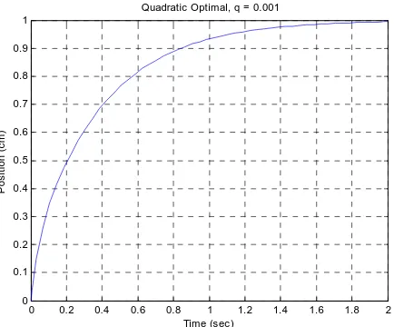
d) Now simulate this system (plant from part c) with a unit step input using the controller and prefilter from part (b). You should get results like those in Figure 3. Turn in your graph.
e) Assume that your fool of a lab partner copied down the numbers incorrectly, and the plant is more accurately modeled as
100 ( )
20 p
G s s
= +
Show (analytically) that the steady state error for the original system for a step input with amplitude A is 0.68A, while the corresponding steady state error for the type 1 system is still 0. Simulate this plant using the original control system (part a) and the modified control system (part b). You should get results like those in Figures 4 and 5. Turn in your graphs.
The moral of this problem is that, if we can, we are usually better off if we do not depend on anything outside the feedback loop! Type 1 system can help alot with modeling errors if we want a zero position error. However, it may take a long time to reach the zero position error.
3) Assume we have the following system
+
-( )
cG s
G s
p( )
where ( ) 1 2 p
G s s
=
+ . We want to design a model matching controller so that • the closed loop system is a second order
• the state error for a step input is zero
• the bandwidth of the closed loop system is 2 Hz.
Luckily I have an uncle who sells good poles cheap, so I obtained a pole at −10π rad/sec for your system. You are to determine the closed loop transfer function (i.e., find the other pole and the numerator) and then the controller to meet these specifications. (Hint:
Read Chapter 7 of the notes!, Ans.
2
40 ( 2)
( )
( 14 )
c
s G s
s s π
π
+ =
4) Consider the following simple feedback system, with which we want to use model matching to determine the controller G sc( ).
+
-( )
cG s
G s
p( )
However, the plant has zeros in the right half plane, and we cannot cancel these poles or we will have an unstable controller. Let's denote the plant
( ) p
G s
( ) ( ) ( )
( )
L R
p
N s N s
G s
D s
=
where we have partitioned the numerator polynomial of the plant into which contains the zeros of the plant in the open left half plane, and which contains the zeros of the plant in the closed right half plane. Let's assume then that the desired closed loop transfer function is written as
( ) L
N s
( ) R
N s
( ) ( ) ( )
( )
( ) ( )
o oo R
o
o o
N s N s N s
G s
D s D s
= =
a) Show that the controller for this system is given by
( ) ( ) ( )
( )[ ( ) ( ) ( )] oo
c
L o oo R
N s D s
G s
N s D s N s N s
=
−
b) Insert the expression for the plant and the expression for the controller from part (a) into the block diagram, cancel where appropriate, and show by simplifying the block diagram that
( ) ( ) ( )
( )
oo R
o
o
N s N s
G s
D s
=
5) Consider the following control system.
pf
G
+-
G s
c( )
( )
pG s
We can compute the position error constant Kp as Kp =Gc(0)Gp(0)
a) Determine an expression for the closed loop transfer function (from input to output) in terms of , , and G .
( ) o
G s Gpf G sc( ) p( )s
b) For a steady state error of zero for a step input we want Go(0)=1. Use this information to show that we can determine the prefilter gain to be
1 1
pf
p
G
K
= +
c) We can find the steady state error for a unit step input as 1
1
ss
p
e
K
=
+ . Using this, show that we can determine the prefilter gain to be
1 1 pf
ss
G
e
= −
Note that if Kp = ∞(or equivalently ess =0), we get Gpf =1. 1)
6) Consider the following control system:
1 1
s
10
s
+
- +
a) If the input to the system is r t( )=8 ( )u t , what is the steady state output?
b) If the input to the system is ( )r t =8sin(3 ) ( )t u t , what is the output in steady state? What is the time lag between the input signal and the output signal?
Hint: you can write ω θ ωt− = (t−td) if θ is measured in radians.
7) The following four plots display the frequency response (magnitude only) for four different systems with real poles. Estimate the settling time for each system.
10-1 100 101 102 -50
-40 -30 -20 -10 0
Frequency (rad/sec)
dB
System A
10-1 100 101 102 -50
-40 -30 -20 -10 0
Frequency (rad/sec)
dB
System B
10-1 100 101 102 -50
-40 -30 -20 -10 0
Frequency (rad/sec)
dB
System C
10-1 100 101 102 -50
-40 -30 -20 -10 0
Frequency (rad/sec)
dB
System D
8) Assume we have the following system
+
-( )
cG s
G s
p( )
where ( ) 1 2 p
G s s
=
+ . We want to design a model matching controller so that • the closed loop system is a second order
• the state error for a step input is zero
• the settling time of the closed loop system is 3 seconds • the percent overshoot of the closed loop system is 20%
. You are to determine the closed loop transfer function and then the controller to meet these specifications.
Ans. ( ) 8.53( 2) ( 2.66) c
s G s
s s
+ =
+
0 0.1 0.2 0.3 0.4 0.5 0.6 0.7 0.8 0.9 1 0
0.1 0.2 0.3 0.4 0.5 0.6 0.7 0.8 0.9 1
Time (sec)
P
o
s
iti
o
n
(
c
m
)
Quadratic Optimal, q = 0.001
0 0.1 0.2 0.3 0.4 0.5 0.6 0.7 0.8 0.9 1 0
0.1 0.2 0.3 0.4 0.5 0.6 0.7 0.8 0.9
Time (sec)
P
o
s
iti
o
n
(
c
m
)
[image:8.612.232.446.74.253.2]Quadratic Optimal, q = 0.001
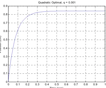
Figure 2. The step response for the new plant and the original controller (Problem 2, part c)
0 0.1 0.2 0.3 0.4 0.5 0.6 0.7 0.8 0.9 1 0
0.1 0.2 0.3 0.4 0.5 0.6 0.7 0.8 0.9 1
Time (sec)
P
o
s
iti
o
n
(
c
m
)
Quadratic Optimal, q = 0.001
Figure 3. Step response of the new plant with the type 1 controller (Problem 2, part d)
0 0.1 0.2 0.3 0.4 0.5 0.6 0.7 0.8 0.9 1 0
0.05 0.1 0.15 0.2 0.25 0.3 0.35
Time (sec)
P
o
s
iti
o
n
(
c
m
)
Quadratic Optimal, q = 0.001
0 0.2 0.4 0.6 0.8 1 1.2 1.4 1.6 1.8 2 0
0.1 0.2 0.3 0.4 0.5 0.6 0.7 0.8 0.9 1
Time (sec)
Po
s
iti
o
n
(
c
m
)
[image:9.612.231.448.75.255.2]Quadratic Optimal, q = 0.001