ISSN Online: 2333-9721 ISSN Print: 2333-9705
DOI: 10.4236/oalib.1104870 Sep. 20, 2018 1 Open Access Library Journal
Research on Point Charge Measurement Model
of Electrostatic Sensor
J. W. Wang
School of Automotive Engineering, Shanghai University of Engineering Science, Shanghai, China
Abstract
In the mathematical model of electrostatic sensors established by Yan Yong in previous studies, the thickness of the insulating layer was not taken into account in the model. In order to study the static monitoring of electrostatic sensors in more depth, this paper considers the influence of insulation layer when establishing the mathematical model of the sensor. By establishing a mathematical model, the point charge measurement model was deduced and formulated. By studying the sensitivity of the sensor, it is concluded that the sensor insulation layer must be considered. The thickness of the insulation layer reduces the sensitivity of the sensor, and the relationship between the sensor spatial sensitivity and the grinding particle size distance is obtained. Compared with the models established by the predecessors, it is concluded that the mathematical model constructed in this paper is feasible and reliable. For the future research of electrostatic sensors.
Subject Areas
Electric EngineeringKeywords
Electrostatic Sensor, Sensitivity Analysis, Point Charge, Mathematical Model
1. Introduction
Aero-engine is one of the most important parts of aircraft. Aero-engine condi-tion monitoring is the guarantee of safe and reliable operacondi-tion of aircraft. In or-der to meet the new requirements of aero-engine fault prediction technology, it is necessary to develop more advanced engine condition detection technology. The electrostatic detection technology can monitor the abrasive particles pro-duced by the wear of parts in the lubricating oil system on-line and warn the en-How to cite this paper: Wang, J.W. (2018)
Research on Point Charge Measurement Model of Electrostatic Sensor. Open Access Library Journal, 5: e4870.
https://doi.org/10.4236/oalib.1104870
Received: August 29, 2018 Accepted: September 17, 2018 Published: September 20, 2018
Copyright © 2018 by authors and Open Access Library Inc.
This work is licensed under the Creative Commons Attribution International License (CC BY 4.0).
http://creativecommons.org/licenses/by/4.0/
DOI: 10.4236/oalib.1104870 2 Open Access Library Journal gine early fault. At present, the work to be done is to improve the measurement accuracy of electrostatic detection technology. Due to the late start of domestic electrostatic monitoring technology and imperfect industrial information, there is still a gap between the aero-engine fault detection technology and foreign countries. At present, the technology has been banned from export, in order to improve the level of domestic aero-engine fault monitoring, domestic research-ers have done a lot of works.
Aircraft engine lubrication circuit electrostatic monitoring technology is based on the principle of electrostatic induction, to on-line detect the debris generated by engine failure. It monitors engine components deterioration at an early stage to prevent engine failure. On-line monitoring of charged debris, predecessors have done a lot of work. Powrie H.E.G. studied the application of electrostatic sensors in aero engine lubrication circuit [1] [2]. And then cooperated with the University of Southampton Wood R.J.K. et al. to study the feasibility of electros-tatic detection in the oil system [3] [4] [5]. Chen Z.X. studied the formation mechanism of charged debris in lubrication system and the principle of oil-line debris electrostatic monitor [6] [7]. Through theoretical modeling and experi-mental verification, Liu R.C. calibrates the parameters of the electrostatic sensor to characterize the nature of the electrostatic sensor [8]. On the basis of Yan’s model, Mao H.J. et al. distributes the charge of the debris evenly on the imagi-nary ring, and simplifies the derivation of the mathematical model [9].
Gajewski J.B. established a three-electrode electrostatic sensor measurement model. The three-electrode electrostatic system consists of debris charge in the sensing zone, the induced charge on the probe, the charge on the electromag-netic screen. Based on the theory of electromagnetism, detected circuit, the charge of the debris and the relationship between charge density and induced potential in the probe are obtained. Using the dynamic charge density and the standard electrostatic charge density which does not change with time, the in-duced potential on the probe is calculated and analyzed [10] [11] [12]. Yong Y.
et al. established the measurement model of the point charge in the electrostatic sensor. Using the Coulomb’s law and the Gauss theorem, the induced potential on the probe is obtained and amplified finally [13]. Xu C.L. analyzed and simu-lated the main factors that affect the performance of the sensor by finite element software ANSYS [14].
In this paper, the electrostatic sensing model is used as the main research ob-ject, and the basic research of the charged abrasive particles in the sensor is car-ried out. The influence of the insulation layer of the sensor on the abrasive ticles monitoring is analyzed, so that the sensor can monitor the abrasive par-ticles more in line with the actual situation and provide a reference for improv-ing the engine fault prediction ability effectively.
2. Principle of Electrostatic Sensor
elec-DOI: 10.4236/oalib.1104870 3 Open Access Library Journal trostatic sensor, electrons will flow inside the metal probe. In order to balance the external charges nearby, the charge inside the probe will be redistributed and accompanied by the electron flow. In this process, there is no charge exchange between the charged body and the electrostatic sensor, and the same amount of charge will be generated on the probe. Then the electrostatic sensor will generate the induced current and convert it into voltage output in proportion. After processing by the conditioning circuit, it will be output to the acquisition system and display. When the charged particles leave the effective induction region of the sensor, the positive and negative induction charges inside the probe will neutralize, making the probe return to be electrically neutral.
3. Physical Model of Electrostatic Sensor
The electrostatic sensor based on the principle of electrostatic induction is shown in Figure 1. The electrostatic sensor is mainly composed of insulating layer, metal probe, shielding cover, amplifier, acquisition card and so on. The probe of electrostatic sensor is usually made of copper. When the charged abra-sive particles pass through the effective range of the sensor, the inductive charge will be generated on the probe. Through the amplifier, the corresponding signal can be obtained from the acquisition card. The insulation layer is made of insu-lating material with very low conductivity, which prevents the transfer of charge between the metal probe and the charged body in the pipeline. In order to re-duce the influence of external environment on the monitoring results of elec-trostatic sensors, a metal shield is installed outside the metal probe to minimize the interference of external conditions and ensure the accuracy of monitoring results.
3.1. Mathematical Model of Point Charge for Electrostatic Sensor
According to the physical model shown above, the electrostatic sensing model of charged abrasive particles is established as shown in the following Figure 2. The axial length of the metal probe is H, the radius is R, and the thickness of the in-sulating layer is r1. It is required that the induced charge produced by the charged abrasive particles on the surface of the probe be set at q. The charge of the charged abrasive particles is Q. The size of the charged abrasive particles is neglected. The inner surface of the metal probe is in close contact with the outer surface of the insulating layer. The coordinate system in Oxyz is established. In this coordinate system, the coordinate of point G is (R + r1, 0, H/2), and the coordinate of metal abrasive particle position P is (x, 0, Z). Point M coordinates in plane xoz (x, H/2), point Q in coordinates OXYZ and point G, point M cop-lanar. According to Figure 3.(
)
(
)
2 2 2
1 2 1 cos
MN = R r+ + OM − R r OM+ φ
Then,
(
)
(
)
2 2 2
1 2 1 cos
DOI: 10.4236/oalib.1104870 4 Open Access Library Journal
[image:4.595.276.470.217.669.2]Figure 1. Physical model of electrostatic sensor.
Figure 2. oxyz coordinate.
Figure 3. oxy coordinate.
[image:4.595.280.468.454.651.2]DOI: 10.4236/oalib.1104870 5 Open Access Library Journal 2 0 4 q E PN πε =
Among them, PN is the distance from P to N.
2
2 2
2
H
PN =Z− + MN
where, MN has been written out before.
The electric field intensity E of charged abrasive q at metal probe N is de-composed. In the oxy plane, the E is decomposed along the ON direction as EM.
sin cos
M
E =E ∠NPM ϕ
Among them,
sin NPM MN PN
∠ =
ONM
ϕ
= ∠Therefore, according to the above formula,
2 0
cos cos
4
M
MN q MN
E E
PN ϕ πε PN PN ϕ
= = Then,
(
)
(
)
(
)
1 32 2 2
2 2
0 1 1
cos
4 2 cos
2
M
q R r x
E
H
z R r x R r x
φ πε φ + − = − + + + − +
According to the Gauss theorem and Coulomb’s law, the total induction charge on the metal probe can be obtained.
(
)
(
)
(
)
(
)
(
)
(
)
(
)
(
)
(
)
(
)
2 10 1 3
2 2 2
2 2
2
0 1 1
1 1
2 2 1
2
0 1 1 2
2 2
1 1
cos
d d
8 2 cos
2
cos 2
4 2 cos
2 cos 2 2 H H
q R r x
Q R r H
H
z R r x R r x
H z
R r q R r x
R r x R r x H
z R r x R r x
H z z π π π φ ε φ πε φ φ π φ φ − − + − = + ⋅ − + + + − + + + + − = ⋅ + + − + + + + + − + − −
∫ ∫
∫
(
)
(
)
1 2 2 2 2 1 1 d 2 cos 2H R r x R r x
φ φ − + + + − +
DOI: 10.4236/oalib.1104870 6 Open Access Library Journal abrasive particles, x is the X coordinate value of the position of the abrasive par-ticles, and angle
φ
is the angle between NO and OP’. V indicates the speed of charged abrasive particles, H indicates the axial length of the metal probe, and r1 is the thickness of the insulation layer.The charged metal particles move along the axial direction of the sensor, and their positions change with time. Assuming that the location of metal particles is unchanged at the X axis and its speed is V, z = vt is known. Therefore, the above formula can be rewritten as follows:
(
)
(
)
(
)
(
)
(
)
(
)
(
)
(
)
1 1
2 2
0 1 1
1
2 2
2 2
1 1
1
2 2
2 2
1 1
cos
4 2 cos
2
2 cos
2
2
d
2 cos
2
R r q R r x
Q
R r x R r x
H vt
H
vt R r x R r x
H vt
H
vt R r x R r x
π φ
π φ
φ
φ
φ
+ + −
=
+ + − +
+
⋅
+ + + + − +
−
−
− + + + − +
∫
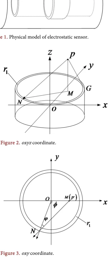
[image:6.595.295.457.561.702.2]It can be seen from the above formula that the induced charge Q produced on the metal probe is related to the distance X between the charged abrasive particle and the central axis of the pipe, the velocity V of the charged abrasive particle, the charged quantity Q of the charged abrasive particle, the thickness R1 of the insulating layer, and the size of the sensor. Through the numerical calculation and analysis of the above formula, we can consider the relationship between each factor and the amount of induced charge with single factor and multiple factors. Below (Figure 4) is a brief diagram of the relationship between the amount of induced charge and time produced by a charged metal abrasive par-ticle passing through the induction zone of the sensor.
DOI: 10.4236/oalib.1104870 7 Open Access Library Journal When the charged abrasive particle passes through the xoy plane as the zero point of time T, −0.1 < T < 0 indicates that the charged abrasive particle enters the effective induction region of the sensor and gradually approaches the xoy
plane, but does not pass through the xoy plane. 0 < T < 0.1 indicates that the charged abrasive particles have passed through the xoy plane and are gradually away from the xoy plane, but are still in the effective induction range of the elec-trostatic sensor. T = 0 indicates that the charged metal grains are on the xoy
plane. The time t [−0.1, 0] does not mean that the time is negative, but that the charged metal abrasive particles are near or far from the xoy plane of the sensor model. As can be seen from the above diagram, when the charged metal abrasive particles are close to the center of the ring probe (xoy plane), the induced charge on the probe increases sharply, and reaches the maximum value when it reaches the xoy plane. When the charged metal abrasive particles are far from the center of the ring probe (xoy plane), the induced charge on the probe decreases sharply, and with the increase of the distance away from the probe, the induced charge on the probe decreases steadily, at this time the induced charge is very small.
3.2. Spatial Sensitivity
Define the spatial sensitivity, the absolute value of the ratio of the induced charge Q produced by the charged metal abrasive particles passing through the induction region of the sensor to the charged abrasive grain q, that is
( )
, QS x z q
=
It is can be obtained
( ) (
)
(
)
(
)
(
)
(
)
(
)
(
)
(
)
1 1 2 20 1 1
1 2 2 2 2 1 1 1 2 2 2 2 1 1 cos ,
4 2 cos
2 2 cos 2 2 d 2 cos 2
R r x
R r S x z
R r x R r x
H z
H
z R r x R r x
H z
H
z R r x R r x
π φ π φ φ φ + − + = + + − + + ⋅ + + + + − + − − − + + + − +
∫
3.3. Spatial Sensitivity Analysis
DOI: 10.4236/oalib.1104870 8 Open Access Library Journal the accuracy of an electrostatic sensor. From the above formula, it can be seen that the sensitivity of the electrostatic sensor is related to the axial length, radial length and insulation thickness of the sensor, and the sensitivity of the sensor is related to the position of the metal abrasive particles.
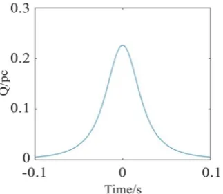
When the size of the electrostatic sensor is determined, that is, H, r1, R remain unchanged, the sensitivity of the electrostatic sensor is only related to the posi-tion of the charged metal abrasive. Select H = 0.02 m, R = 0.01 m, r1 = 0.001 m, z
= 0. Simplify the above formula.
(
)
(
)
2 2(
)
12
0 2 2
0.011 0.011 cos 0.02
, 0 d
4 0.011 0.022 cos 0.0001 0.011 0.022 cos
x S x z
x x x x
π φ
φ
π φ φ
−
= = ⋅
+ −
+ + −
∫
The following Figure 5 can be roughly obtained by introducing the size value of the sensor (roughly given the size of the sensor, not the best size).
The relationship between the sensitivity of the electrostatic sensor and the radial position of the charged metal abrasive particles can be clearly seen from the above diagram. When the radial position of the charged metal abrasive par-ticles is zero, that is, on the Z axis of the pipe center, the sensitivity of the elec-trostatic sensor is the lowest. When the radial distance is 0.01, the sensitivity of the sensor is the highest on the inner surface of the insulation layer. This situa-tion is consistent with the physical characteristics of electrostatic inducsitua-tion.
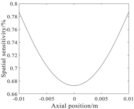
[image:8.595.264.484.525.703.2]The sensitivity of the electrostatic sensor without considering the thickness of the insulating layer is S1, and that of the electrostatic sensor with considering the thickness of the insulating layer is S2. The reason for the difference between the two sensitivities is that the thickness of the insulating layer in the sensor is taken into account when establishing the charged abrasive particle model, which is also a factor that must be considered in the design of the electrostatic sensor. As shown in Figure 6, the sensitivity of S2 is close to the value of S1 as the insula-tion thickness decreases. When there is no insulating layer at all, S1 will com-pletely overlap with S2. The trend of the two curves is exactly the same, and the
DOI: 10.4236/oalib.1104870 9 Open Access Library Journal
Figure 6. Comparison of two spatial sensitivities.
difference between the two sizes is not significant. It shows that the model estab-lished in this paper is reliable and feasible.
4. Conclusions
1) The mathematical model of the electrostatic sensor is established, and the influence of the insulation layer of the electrostatic sensor is considered. The mathematical model is derived in detail. The sensitivity index of sensor is de-fined, and the space sensitivity curve of electrostatic sensor is obtained.
2) The sensitivity of the sensor is analyzed, and the relationship between the spatial sensitivity of the sensor and the orientation distance of the grinding par-ticle is obtained. In the center line of the sensor axis, the space sensitivity of the electrostatic sensor is the lowest. Along the pipe radius, the space sensitivity in-creases gradually to the pipe wall, and the space sensitivity is the highest over the pipe wall.
3) The location of charged abrasive particles and radial radius of the sensor are studied by comparing with the model established by predecessors, and the spatial sensitivity curves are verified by each other. The accuracy and reliability of the mathematical model of the electrostatic sensor are illustrated.
Conflicts of Interest
The authors declare no conflicts of interest regarding the publication of this pa-per.
References
[1] Powrie, H.E.G. (2000) Use of Electrostatic Technology for Aero Engine Oil System Monitoring. Proceedings of IEEE Aerospace Conference 2000, Big Sky, MT, March 2000, 57-72. https://doi.org/10.1109/AERO.2000.877883
DOI: 10.4236/oalib.1104870 10 Open Access Library Journal [3] Harvey, T.J., Wood, R.J.K. and Powrie, H.E.G. (2007) Electrostatic Wear
Monitor-ing of RollMonitor-ing Element BearMonitor-ings. Wear, 263, 1492-1501.
https://doi.org/10.1016/j.wear.2006.12.073
[4] Wang, L., Wood, R.J.K., Harvey, T.J., et al. (2003) Wear Performance of Oil Lubri-cated Silicon Nitride Sliding against Various Bearing Steels. Wear, 255, 657-668.
https://doi.org/10.1016/S0043-1648(03)00045-0
[5] Morris, S., Wood, R.J.K. and Harvey, T.J. (2002) Use of Electrostatic Charge Moni-toring for Early Detection of Adhesive Wear in Oil Lubricated Contacts. Journal of Tribology, Transactions of the ASME, 124, 288-296.
https://doi.org/10.1115/1.1398293
[6] Chen, Z.X., Zuo, H.F., Zhan, Z.J., et al. (2012) Study of Oil System Oil-Line Debris Electrostatic Monitoring Technology. Acta Aeronautica Et Astronautica Sinica, 33, 446-452.
[7] Chen, Z.X., Zuo, H.F., Zhan, Z.J., et al. (2012) Method for Oil-Line Debris Electros-tatic Monitoring of Bearing Steel Sliding Friction Pairs. Journal of Aerospace Power, 27, 1096-1104.
[8] Liu, R.C., Zuo, H.F., Sun, J.Z., et al. (2017) Simulation of Electrostatic Oil Line Sensing and Validation Using Experimental Results. Tribology International, 105, 15-26. https://doi.org/10.1016/j.triboint.2016.09.026
[9] Mao, H.J., Zuo, H.F., Huang, W.J., et al. (2016) Mathematical Modelling and Cali-bration Experiment of New Electrostatic Sensor in Aviation. Acta Aeronautica Et Astronautica Sinica, 37, 2242-2250.
[10] Gajewski, J.B. (1997) Dynamic Effect of Charged Particles on the Measuring Probe Potential. Journal of Electrostatics, 40-41, 437-442.
https://doi.org/10.1016/S0304-3886(97)00084-3
[11] Gajewski, J.B. (1997) Electric Charge Measurement in Pneumatic Installations. Journal of Electrostatics, 40-41, 231-236.
https://doi.org/10.1016/S0304-3886(97)00042-9
[12] Gajewski, J.B. (1989) Continuous Non-Contact Measurement of Electric Charges of Solid Particles in Pipes of Pneumatic Transport. I. Physical and Mathematical Mod-els of a Method. Conference Record of the IEEE Industry Applications Society An-nual Meeting, San Diego, 1-5 October 1989.
[13] Yan, Y., Byrne, B., Woodhead, S., et al. (1995) Velocity Measurement of Pneumati-cally Conveyed Solids Using Electrodynamic Sensors. Measurement Science & Technology, 6, 515-537. https://doi.org/10.1088/0957-0233/6/5/013
[14] Xu, C.L., Wang, S.M., Tang, G.H., et al. (2007) Sensing Characteristics of Electros-tatic Inductive Sensor for Flow Parameters Measurement of Pneumatically Con-veyed Particles. Journal of Electrostatics, 65, 582-592.