Comparative Assessment on the Performance of
Open-Loop and Closed-Loop IFOGs
Mohammad Reza Nasiri-Avanaki1, Vahid Soleimani2, Rohollah Mazrae-Khoshki2
1Electronics Department, Azad University of Karaj, Tehran, Iran 2Electronic Engineering Department, RAZI University, Kermanshah, Iran
Email: [email protected]
Received January 5, 2012; revised February 7, 2012; accepted February 17, 2012
ABSTRACT
In this paper, we evaluated comprehensively the structure and operation of open-loop interferometric optical fiber gy-roscopes (IFOG). To complete the previous works, a digital approach to derive the rotation angle in optical fiber gyro-scopes is investigated theoretically. Results are simulated by the MATLAB software; therefore we could compare the results in simulated area with the values derived from theory. Also, feedback Erbium-doped fiber amplifier (EFDA) FOGs, called FE-FOG, is categorized in closed-loop IFOGs. The procedure of finding the Sagnac shift for open-loop and closed-loop IFOG have been studied and compared to one another. The signal processing in the open-loop IFOG was simulated using Matlab software and for the closed-loop IFOG by PSCAD. In the open-loop IFOG the analogue formulation of the IFOG in order to extract the phase shift is analyzed. A novel and promising method for derivation of Sagnac phase shift based on digital finite impulse response filtering is proposed. Based on our simulation results, the reliability and accuracy of the method is determined. In the closed-loop IFOG, the shift was derived through frequent use of Sagnac loop. The output signal is injected in the input again as feedback. The shift phase between clockwise and counterclockwise waves in each complete route, including primary and feedback route, is identified as Sagnac shift phase.
Keywords: Feedback Erbium-Doped Fiber Amplifier FOG (FE-FOG); Erbium-Doped Fiber Amplifier (EFDA); Digital Signal Processing; PSCAD; FIR Digital Filters; Interferometric Fiber Optic Gyro (IFOG); Sagnac Shift
1. Introduction
Angular rotation in vehicles is one of the parameters that need to be accurately measured in order to describe the position of an object. Traditionally, the angular momen- tum of a spinning rotor was used to determine the angu- lar rate or displacement [1-3]. These devices are suscep- tible to damage from shock and vibration, exhibit cross- axis acceleration sensitivity and, for the lower cost ver- sions; they have reliability problems [3].
Directions around the same closed optical path will experience path length difference that is proportional to the rotation rate of the setup [4,5]. Sagnac shift is the common feature among optical gyros. Sagnac is now extensively used in commercial inertial navigation sys-tems for aircraft. Given the advantage of this effect, the actual path length difference due to the rotation is quite small, e.g. the gyro used in the aircraft navigation must detect rotation rates below 0.01 deg/hr [6]. FOG is used for measurement of the rotation based on Sagnact Effect. Two types of FOG are used: the interferometric FOG (I-FOG) in which a low coherence light source is used
and the resonance FOG (R-FOG). In the R-FOG the dif-ferences of resonance frequency caused by sagnact effect is utilized for measuring the rotation. Therefore even a short length of optical fiber is sufficient for the meas-urement. R-FOG needs a coherent light source for which such effects like Kerr effect and reflective optic phe-nomenon must be considered. The FOG converts the Sagnact phase shift into a beam frequency between the clockwise and counterclockwise of laser modes. This implies sensing path length changes of about one part in 1016, which corresponds to absolute length changes on
the order of a nuclear dimension. Requirement of the precision of rotation measurement for spacecraft naviga-tion lies between 0.01˚/hr to 0.001˚/hr.
The principle of operation of a typical fiber gyro is based on a phase modulation in both directions of an optical fiber loop, as if it acts as a delay line. The modu- lation frequency, 1
2
P
f
the returning power is not perfectly stable.
Ring laser gyroscope (RLG) consists of a ring laser having two counter-propagating modes over the same path in order to detect rotation. It works based on Sagnac shift effect and requires high vacuum and precision mir- ror technology, which makes this technique very expen- sive [4]. The physical principal of RLG operation is ana- logous to the Doppler Effect, but it involves determina- tion of the phase shift between two counter-propagating light beams in an evacuated mirrored cavity [6]. To ad- dress this drawback, interferometric fiber optic gyro (IFOG) is employed whose function resembles RLG, notwith- standing the fact that, in IFOG, the same effect is ob- tained in a fiber coil with the elimination of the high voltage and high vacuum, which results in a low-cost inertial rotation sensor [4,6]. In addition, IFOGs are ab- stracted in miniature devices; all-solid state with a lim- ited number of components, therefore lower cost.
In terms of light source, RLG requires an external narrow band gas laser with its active gain medium which is an integral part of the sensing cavity, whereas IFOG works with an external broadband light source [7]. Path length measurement in RLG is performed by measuring the difference of resonant frequencies between two cavi-ties [5]. Despite, IFOG rotation rate sensing is achieved through a direct measurement (open loop) or nulling (close loop) of the optical phase difference due to the rotation-induced Sagnac phase shift [4,6,7].
According to the fact that high precision gyro is not always required, e.g. in land automotive vehicle an IFOG with the accuracy between 10 to 200 deg/hr is sufficient [8], and also regarding to the least requirements with the most flexibility in the design of IFOG, the improvement of this sensor becomes more sensible.
2. Principle of Operation
The principle of operation of an IFOG is based on the phenomenon that a circuital system has different optical path lengths in the two propagation directions when it rotates [9]. The difference between counter propagating beams provides the amount of the rotation. The main structure includes a laser diode, usually a super lumines-cent diode (SLD) or Rare-earth doped fiber with im-proved wavelength stability, a coupler to split light into clockwise and counterclockwise directions, a length of optical fiber wound on a coil as the rotation sensing loop, and a photo detector to convert optical information into electrical signals for further processing. Light source tem- perature is controlled by using a thermo electric cooler (TEC) and the detector is a PINFET module with a high sensitivity and hybrid trans-impedance amplifier. The type of the fiber optic and the way of winding specify the par- ticular category that IFOG belongs to, which suits it to
the specific application of the sensor [10]. A complete IFOG has identical optical paths in the clockwise and counter clock wise. In this IFOG known as “minimum configuration”, a polarizer and second coupler are em- ployed [5,11].
Optical signal is received by the detector after passing through the fiber coil and couplers and converted into the electric current. An electrical amplifier is connected to the detector to change the current to the appropriate vol- tage. The obtained voltage is, then, amplified and fed into the signal processing circuit to extract the angular rotation rate [5,12].
EF-FOG work by frequent utilize of sagnact loop, in this manner output signal re-inputted as feedback. It per-forms like R-FOG but without high length coherence light source and never use the resonance effect. FE-FOG in comparison with Open-loop I-FOG has high sensibil-ity and wide dynamic range. In this paper we compare the results of open loop and closed loop I-FOG.
A light source with a coherence length much shorter than the coil length allows only the wave pairs that have circulated the same number of times in the loop to inter-fere with each other and to produce an output related to the rotation-induced nonreciprocal phase shift. The re-sultant optical response is essentially the sum of all the optical responses of a series of conventional Sagnac In-terferometric fiber-optic gyroscopes with their effective loop length in multiples of a single coil’s length. The multiple-trip interference and the associated intensity summation produces a response resembling a resonance phenomenon, with the strength and sharpness of the resonance increasing with the number of interfering light waves. The proposed gyro has different from a resonant fiber-optic gyro (R-FOG) because it uses a low coherent light source. The low coherent source minimizes not only errors from Rayleigh back scattering, but also bias errors caused by the optical Kerr effect. This could not possibly be done in an R-FOG because of high coherent light source.
If the modulation frequency of phase modulator in sagnact loop consists of whole loop time delay, the out-put signal in IFOG will be in pulse shape; therefore, when rotation occurs in the system, the location of output peak pulse shifts by sagnact effect. Precision of meas-urement depends on sharpness of the output pulses. Sharpness of output pulse is determined by the phase modulation depth and EFDA gain.
Miniature fiber optic gyros have also been manufac-tured with all solid-state optical devices for precise meas- urements of mechanical rotation based on the sagnac principle.
al-though used for different tasks.
3. Rotation Equation
When the optical ring is rotated with a tangential velocity
, the beam rotating with the ring will have an optical path longer than the counter-rotating beam by a distance
given by [1]: L
4πR L
c
(1) where, R is the ring radius and c is the speed of light in the vacuum. For a monochromatic light of wavelength
, this change in optical path length results in the Sagnac phase difference, which is given by Equation (2).
2
2π 8π R L
c
(2)
The phase difference between two beams, after pass- ing the ring with the area A and rotating with an angular velocity , generates a phase difference which is given by [1]:
8πA c
(3) It is important to note that, the resultant phase shift is independent of the medium and of the exact shape of the loop. This compliant property of the IFOG is an ad- vantage when it is required to design it to fit the volume constrains in the specific applications [1]. However, the resultant phase shift can be increased by additional loops (turns of fiber) i.e. if it is wound N turns of the fiber coil. The resultant phase shift becomes [13]:
8πA N c
(4) Alternatively, we can express the resultant phase shift in terms of coil diameter and fiber length by noting that:
2
π 4
D
A (5) And,
π
LN D (6) So, the Sagnac phase shift can be rewritten as:
2πLD c
(7)
As one example in a typical IFOG (200 m coil length, 10 cm-diameter coil) for measurement of the earth angular rotation ( = 15˚/h = 0.73 µr/s), the sensor detects a phase difference of = 36 µr, correspond- ing to an optical path difference of the order of 10 - 12 m [2,13].
Eventually the output signal for such configuration will be [2]:
0
1 cos
I t I
in which, I0 is the current obtained when the ring is at
the rest.
4. Open-Loop Configuration with Phase
Modulation
As mentioned above, the major problem of the basic configuration is the output nonlinearity for small phase shift, s 0 which hinders high sensitivity measure-ments of the small rotation angles [14]. This limitation is overcome by transforming the base band cosine-depen- dence into a sinusoidal function [1,3]. Although for translating the output signal from base band to a carrier at angular frequency mod, different solutions have been
proposed, but today optical phase modulation technique is commonly used. The typical setup of a practical IFOG in all-fiber technology has a phase modulator which is inserted in the fiber coil close to a coupler output so that the phase delays are cumulated by the counter propagat-ing waves. In all-fiber IFOG, phase modulator is con-structed by winding and cementing a few fiber turns on a short, hollow piezoceramic tube (PZT). By applying a modulating voltage to the PZT, a radial elastic stress and a consequent optical path length variation due to the elasto-optic effect are generated [14].
5. The Open-Loop IFOG Modulation
Equation
In this section, the modulation equations of extracting the phase shift are comprehensively described. In the con-figuration described in the previous section, the clock-wise (CW) and counterclockclock-wise (CCW) propagating waves experience a phase delay
t and
t
, respectively [15], where L v is the radiation transi-tion time in a fiber with an overall length . By apply-ing a phase modulation at angular frequencyL
mod
, the modulation equation will be [16]:
mod t mod,0cos modt mod,0cos 2πmod
f t
(9)Here, mod,0 is the amplitude of modulation signal,
and fmod is the modulation frequency.
Therefore, CW and CCW waves are modulated as phase shift by mod
t and mod
t
, respectively.So, the modulation phase shift difference is as follows:
mod t mod t mod t
(10) Finally, the total phase shift in the output signal will be:
mod mod
total ccw cw t t
(11)
Now, the output signal will become:
0
1 cos
mod
0
1 cos
total
I t I t I
(12)
Considering the fact that the SLD switched by 1 2
p
f , with the help of Equations (9), (11) the phase shift becomes [16]:
mod mod,0 mod
mod,0 mod
cos 2π
cos 2π
t f
f t
t
(13)
mod mod,0 mod mod
mod mod
mod,0 mod
2 sin π sin 2π
2
π π
2 sin sin 2π
2 p 2 p
t f f
f f f t f f t (14) Substituting the amplitude with Equation (15) as fol-low [1]: mod mod,0 π 2 sin 2 MI p f f
(15)
The output current of photodiode becomes:
mod0 mod
π 1 cos sin 2π
2
MI
p
f
I t I f t
f (16)
Or can be rewritten as:
mod 0 mo mod mod π 1 cos cos sin 2π2
π sin sin sin 2π
2 MI p MI p f
I t I f t
f f f t f d
(17) Using the below Bessel equations:
0
2
1
cos sin 2 m cos 2
m
x s J x J x ms
(18)
2 1
1
sin sin 2 m sin 2 1
m
x s J x m
s (19)Equation (17) can be rewritten in a way that one can easily extract the relevant harmonics [16]:
0 0 2
1 mod mod 2 1 1 mod mod
( ) 1 cos 2
π cos 2 2π
2
sin 2
π cos 2 1 2π
2
MI m MI
m
p
m MI
m
p
I t I J J
f m f t
f
J
f
m f t
f
(20)To have an optimum sensitivity, output power, photon noise, and signal to noise, MIis selected to be as [16]
1.85 radMI opt
(21) To simplify Equation (20), we consider fmod = fp [1,16].
Using this assumption and Equation (15), we will have:
mod,0 mod,0
2 0
MI opt
.925 (22) The amplitude of the output signal at fmod, which gives
the first harmonic of the output current, i.e. Equation (20) will be [2]:
modmod 1 0 1 mod,0
π
2 sin 2 sin
2 p
f
I f C I J
f
(23)
p mod
2 1 0sin
1
2 mod,0 [image:4.595.59.534.102.740.2] [image:4.595.309.538.623.737.2]I f f C I J
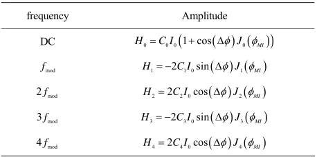
(24) Table 1 shows the four harmonics generated in the photodiode output current [2]:Now, we can calculate by H1 with the below
equation [2,16]:
1 0 1 arcsin 2 MIi H CI J (25)
Could be also obtained with another approach using H1, H2, J1 and J2 [16]:
1 2 2 1 arctan MI MI H J H J (26)
A comfort and reliable method is proposed here is to use H1, H2, H3 and H4 to calculate with the help of
the solution of Equation (27) and Table 1 [2,16]:
1
1
2
m m m
m
J x J x J x
x (27)
2 2 4 4 MI MI J H H J (28)
2 1 3 4 tan MI HH H
(29)
Table 1. Harmonics of the photodiode output current. Ci =
C, i = 0, ···, 4.
Amplitude frequency
0 0 0 1 cos 0 MI
H C I J
DC
1 2 1 0sin 1 MI
H C I J mod
f
2 2 2 0cos 2 MI
H C I J mod
2f
3 2 3 0sin 3 MI
H C I J mod
3f
4 2 4 0cos 4 MI
H C I J mod
3 2 4
6 1
tan
MI
H
H H
(30)
Owing to this, the Sagnac shift is obtained as Equation (31) which is the best suited for hardware implementa-tion:
3 1 3 2 2 4 3
arctan 2
H H H
H H H
(31)
6. Evaluation of Digital Filtering in an
Open-Loop IFOG
The simulation results of the abovementioned procedure show that, this approach can perfectly be employed in the signal processing part of IFOGs. To achieve the required harmonics, four digital filters are designed. These filters were designed by SPtool in Matlab 7a. Since the phase linearity of the filters was important, finite impulse re-sponse (FIR) filters were taken into account to have the four required band pass filters. Regarding to the available data the beneath quantities are listed as input of the simulation:
Input rotation rate = 10 deg/s (AHRS range); Coil length = 500 m;
Coil diameter = 10 cm;
Sampling frequency = 10 MHz; Time domain = 2 ms;
Wave length = 1310 nm;
Refractive index of optical fiber core = 1.43; Coil length transient time = (500/3e8) × 1.43. The coil frequency is obtained as
1 2 1 2L c1.43 0.208 MHz. As mentioned before, this frequency is the PZT vibration and SLD switch fre-quency, as well.
Figure 1 shows the designed band pass filters with the same bandwidth (0.208 MHz) but different central fre-quencies. In the filters in Figure 1, Fp and Fs are, pass
band frequency and stop band frequency, respectively. Also, Rp and Rs are ripples in pass band and stop band.
The filters are described as follows:
1) Band pass filter: Gain = 1, central frequency = 0.208 MHz;
2) Band pass filter: Gain = 1, central frequency = 0.416 MHz;
3) Band pass filter: Gain = 1, central frequency = 0.624 MHz;
4) Band pass filter: Gain = 1, central frequency = 0.832 MHz.
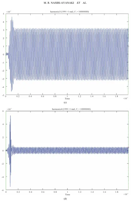
To extract the four harmonics from the IFOG output current, the filters are implemented by considering the direct form structure. Figure 2 shows the amplitude of the filtered signals, H1 to H4. In the next step, rotation
rate , is calculated using H1 to H4 with the help of
Equations (7) and (31).
The comparison of calculated with the input rota-tion rate, i.e. 10 deg/s showed one percent difference. This discrepancy caused from utilizing unsharp filters. As it has been experienced, we will reach to the better accuracy if higher order filters are considered.
7. Closed-Loop EF-FOG Configuration and
Operation
In this structure the weak feedback signal is amplified by the Er-Doped Fiber Amplifier (EDFA) to prevent the laser scattering. Fiber amplifier is assumed to be linear, which means there are no gain effects. The output signal is the sum of interferometric CW and CCW beams in the total route. The modulator is located in sagnac loop. If the phase modulator frequency is selected properly, the output signal will be a series of short pulses [17]. Hence modulation frequency of phase modulator and route de-lay must be approved by the equation m 2nπ where
m is angular frequency of the phase modulation, and
is the time delay in whole round trip loop consisting of Sagnac loop and amplified fiber optic loop. If the sharpness of output pulses could not be adjusted by phase modulation, by changing EFDA gain it can be compen-sated. If this equation m 2nπ0 is not realized, for
example due to detuning, there will be a phase shift 0
that can be demodulated as an error signal for phase modulated (PM) technology. The operation of the FE- FOG is sensitive to the EDFA gain [18]. In theory the first intereferometric output signal without feedback is equal to ordinary IFOG as:
1 1
2 π 1 cos s ecos m
m n P t K v t
(32) where v is the interferometric coefficient and K1 is a
pa-rameter that expresses the loss resulting from the Sagnac loop and the couplers of the Sagnac interferometer, m
is the modulation frequency, e is the effective phase-
modulation depth, which is expressed as
2 sin π
e m fm s
(33)
s
is the wave-propagation time through the Sagnac loop (please note the difference with the total time round- trip delay t) and is expressed as s nL c (where L is
the length of Sagnac loop), and m is the phase-modu-
lation depth. s is the Sagnac phase shift induced by
rotational movement, which is expressed as Equation (7) in the previous section.
By considering the effect of optical feedback, the sec-ond-time interference signal experienced after the feed-back has been derived is
2
2 1 2 1 cos cos
1 cos cos
s e m m
s e m
P t AK K v t
t
(a)
(c)
[image:7.595.87.513.85.647.2](d)
Figure 1. Band pass filters for extracting four harmonics from the photocurrent IFOG signal. FIR filter design is taken into account as these filters have phase linearity. (a) Band pass filter (harmonic 1) Kaiser window FIR with order = 100, Fp1 =
0.202 MHz, Fp2 = 0.21 MHz, Fs1 = 0.334MHz, Fs2 = 0.399 MHz, Rp = 0.3917, Rs = 39.45, Phase Delay = −0.255 rad; (b) Band pass filter (harmonic 2) Kaiser window FIR with order = 153, Fp1 = 0.4 MHz, Fp2 = 0.43 MHz Fs1 = 0.249 MHz, Fs2 = 0.587
MHz, Rp = 0.3276, Rs = 40.97, Phase Delay = −1.159 rad; (c) Band pass filter (harmonic 3) Kaiser window FIR with order = 162, Fp1 = 0.597 MHz, Fp2 = 0.653 MHz, Fs1 = 0.457 MHz, Fs2 = 0.802 MHz, Rp = 0.33, Rs = 40.29, Phase Delay = −0.361 rad; (d) Band pass filter (harmonic 4) Kaiser window FIR with order = 148, Fp1 = 0.802MHz, Fp2 = 0.849MHz, Fs1 = 0.650 MHz, Fs2 =
(a)
(c)
[image:9.595.87.510.53.703.2](d)
and the third-time interference signal that occurs after feedback has been twice derived is
2 2 3 23 1 2 1 cos cos 2
1 cos cos
1 cos cos
s e m m
s e m m
s e m
P t A K K v t
v t v t (35) where A is the gain of the fiber amplifier and K2 is a
pa-rameter that depends on the coupling ratio of the feed-back couplers and the transmission loss in the feedfeed-back loop. For simplicity, we assume that K K K1 2. The
total output at the photodetector is the summation of the number of above-mentioned interferences and is ex-pressed as
1
2
3
total
P t P t P t P t (36) If m 2nπ, the total photodetector output can be realized by proper adjustment of the modulation fre-quency to match the round-trip time, and we can have
1 cos cos
1 1 cos
s e m
total
s e m
K v t
P t AK
t
,
(37)
where K is the photodetector coefficient, because the total output is a series of short pulses, we can determine the peak value through the following equation:
0
sin cos 0
cos 2 π, 0,1, 2,3
total
s e m
s e m
P t
Kv t
t n n
(38)
Above Equation is a condition required to find the peak position of the output pulse that is valid for both cases of rotation and nonrotation, please note that only those equations of even p correspond to the peak position. From this equation and condition we can see that the output pulse shifts if rotation occurs.
For Open-Loop Method for the FE-FOG In Equation (33) if e is selected to be between 0e2π and
0
s
there is no rotation, Equation (33) is satisfied only when n = 0. In this case, the peak positions of the output pulse are determined through the following equa-tion:
0 2 1
π, 0,1, 2, 2
m
i
t i
(39)
Here 0 represents the peak positions corresponding to the nonrotation case and i denotes the peak number of the output pulse in the time axis. We see that the peak positions are not affected by the phase-modulation depth
t
e
when there is no rotation. On the other hand, when
rotation occurs (s0) the peak positions are affected by the Sagnac phase shift and can be determined by
arccos
m r 2π, 0,1, 2, s
e
t i i
(40)
where r denotes the peak positions when rotation
oc-curs and i has the same meaning as in Equation (39) Comparing Equations (39) and (40), we see that the peak positions shift if rotation occurs, and the shift of the peaks is just equal to r 0
t
t t t
. Therefore, the peak
positions are in fenced by only the Sagnac phase shift if rotation occurs and if we fix the phase-modulation depth
e
. We can thus determine the rotation rate by the detec-tion of the peak shift t of the output pulse.
In this paper the wave-length of optical source is
0 1.5μm
, the modulation frequency of the phase modulator, fm0.209790 MHz (m2πfm
rad
), and the radius of the Sagnac loop is R = 0.05 m. The round-trip length is 500 m, which is selected to match the modulation frequency for the pulse output, of which the Sagnac-loop length is 460 m and the length of the EDFA (including the pigtail of couplers) is 40 m. The interfer- ometric coefficient is v = 0.96, the photodetection coeffi- cient is K = 0.2, the parameter K = 0.06, the effective phase-modulation depth is e0.6 , and the Sagnac
[image:10.595.311.536.545.716.2]phase shift is s0 for the nonrotation case.
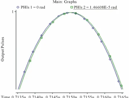
Figure 3 demonstrates the principle of the rotation measurement for the open-loop method when the output pulse is shifted by rotation. The plots are normalized and
0.18 rad
e
. We see that the peak position shifts if ro-tation occurs, phase shift 0˚/h and 3.6˚/h. Further calcula-tions show that the shift is increased as the rotation rate increases. The very sharp peak of the output pulse can result in a high-resolution rotation measurement. From Equations (7) and (38)-(40) (in Equation (39), i = 0, 2, 4), we can derive the rotation rate as:
0
0 0
cos 4π
sin 4π
e m m
e m
c
t t
RL c
t RL
(41)
where is the time shift of the output peak as a result of the rotation, In Closed-Loop Method for the FE-FOG, we selected e
t
with a condition of 2πe 4π. In
such a case the output pulse is shifted by only the rota-tion. In this section, we hope to show that the output pulse is affected by both rotation and phase modulation, so that we can use the phase modulation to compensate the Sagnac phase shift. Such a technical idea is consistent with the closed-loop method.
In Equation (38), if we assume that s 0 (nonrota-tion) and we select 2πe4π, e.g., e 2.2π, then
Equation (38), can be satisfied by n = 1, n = 0, and n =
[image:11.595.140.458.439.703.2]−1, which means that the output pulse has three kinds of peaks. The peaks corresponding to n = 0 have the same properties as do those of the open-loop method and will not be affected by the phase modulation; however, the peaks corresponding to n = 1 or n = −1 will be in fenced by both the Sagnac phase shift and the phase-modulation depth. This performance can be used for the rotation measurement.
Figure 4 shows that the output pulses related to 0.2π
e
2.2π
e
is simple, but, the output pulses related to
are complicated and consist of three kinds of
peaks designated A, B, and C. (Note: if we select e to
be greater than , even more output peaks will appear, because in Equation (38) n also includes integers over. This case can also be analyzed similarly). The peak posi-tions for A, B, and C are determined by n = 1, 0, −1, re-spectively, in Equation (38). In this paper, we look at the peak positions corresponding to peaks A (peaks C also have similar properties). In one time period, peaks A also consist of two additional peaks, marked with circles and squares, whose positions are determined by
4π
arccos 2π 2 π
2π arccos(2π ) 2 π 0,1, 2,
m A e
m A e
t n
t n n
(42)
N = 0, 1, 2, ··· respectively. If the Sagnac phase shift induced by rotation is canceled by the phase modulation of the phase modulator, the peak positions corresponding to peaks A will not shift in spite of rotation’s occurring. To realize this phase compensation we can feed back an electrical signal at the phase modulator. The rotation rate can thus be evaluated through the value of the phase modulation. Further calculations also show that, although in the closed-loop case (when both rotation and feedback control of e occur) peaks B and C are shifted, they
cannot cross with peaks A. This is because, for in any case, the peak positions of peaks A, B, and C are deter-mined from Equation (38) with n = 1, 0, −1, respectively, and they always have different values. The above result
Figure 4. show the comparison of the output pulses for different phase modulations when one value of e, 0 e 2 and
lls us that dynamic range is
ore detailed mathematical description is presented in
te in the closed-loop case the large.
A m
the following paragraphs. We first consider the case of nonrotation ( s 0, for which the peak positions corre-sponding to p can be determined by
0cos 2π
e m At
eaks A
(43) where is the phase-modulation dep
(44)
and from Equations (43) and (44) we can further derive
0
e
onr
th corresponding to the n otation case. On the other hand, when rotation occurs and if the electrical-feedback signal is placed on the phase modulator, the peak positions corresponding to peaks A will not change, and we then have
0
2π cos ,
s e e m At
0
cos 2π e,
t
s e m A
e
(45)
We can evaluate the rotation rate by detecting e.
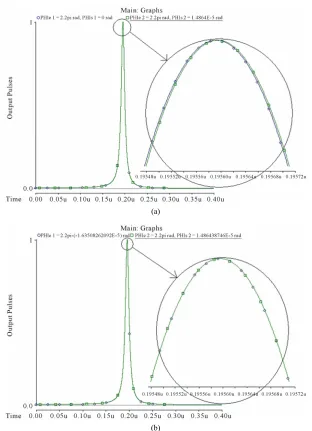
[image:12.595.142.454.269.700.2]dula Figure 5 shows the variation of the phase-mo tion depth e as a function of the rotation rate for the closed
loop. Fi re 5(a) shows the output pulse when the rota- tion doesn’t exist 0
gu
and e e02.2π and Fig-
ure 5(b) shows th put pu e without
electric feedback signal in phase modulator Ω = 3.65˚/h and e e0 2.2π
e out lse when rotat
therefore when rotation occur out-put pul n see the peak that shifted by rotation could back to the first position that e
ses shifted. We ca
shows the variation of phase modulation induced by electric
(a)
(b)
Figure 5. (a) Output pulse when the rotation doesn’t exist 0 and e e02 2.; (b) output pulse when rotate without
electric feedback signal in phase modulator Ω = 3.65˚/h and e e02 2..
feedback, that means the rotation rate of Ω = 3.65˚/h needs the phase compensation
1.63508262092E 5
e
.
8. Conclusions
prehensive formulation of open loop
o
REFERENCES
[1] M. Nasiri-Ava Digital Signal Pro- In this paper, a com
interferometric fiber optic gyroscope (IFOG) was studied. Through the signal processing explanation, an accurate approach was proposed to calculate the phase shift to make the hardware implementation simpler. The simula-tion results of the digital signal processing using FIR filters showed that the chosen computational method to extract Sagnac shift from IFOG signal current is promis-ing. With pointing out the similarities and differences between calculated with the input rotation rate of 10 deg/s, and the output f the digital filtering approach, just a slight difference of less than 1% was observed. This distinction appeared because of using unsharp filters. Re- garding to the experiences, we will have more accurate IFOG if higher order of filters are utilized.
Also the functionality of the closed-loop fiber-optic gyroscope (I-FOG), based on multiple utilizations of the Sagnac loop and amplified optical feedback, has been proposed and theoretically investigated. The new gyro-scope is termed as feedback Er-doped fiber-optic ampli-fier (FEDFA). A low-coherence light source is used in this FOG [19]. Amplification of a weak feedback gyro-scope signal is performed by the incorporated EDFA. The final gyroscope output is pulsed if the modulation frequency of the phase modulator matches the round-trip time [20]. Sagnac phase shift can induce a shift of the output pulse, which is used for the rotation measurement.
naki, “Full Progress of
cessing in Open Loop-IFOG,” IEEE Optical Fiber Com- munication & Optoelectronic Exposition & Conference, Shanghai, October 2006, pp. 1-10.
[2] M. Nasiri-Avanaki, “Digital Filtering to Obtain Sagnac Shift in Open Loop-IFOG,” North American Radio Sci-ence ConferSci-ence, Ottawa, July 2007, pp. 23-29.
[3] S. Merlo, M. N. Orgia and S. Donati, “Fiber Gyroscope Principles,” Handbook of Fibre Optic Sensing Technol-ogy, John Wiley & Sons, Ltd., Hoboken, 2000, pp. 1-23. [4] H. C. Lefevre, “Fundamentals of the Interferometric Fiber-
Optic Gyroscope,” Optical Review, Vol. 4, No. 1a, 1997, pp. 20-27. doi:10.1007/BF02935984
[5] M. Nasiri-Avanaki, “Open Loop-Interferometric Fiber Optic Gyroscope: Analysis and Methods to Implement,” M.Sc. Thesis, Semnan University, Semnan, 2006. [6] S. Oho, H. Kajioka and T. Sasayama, “Optical Fiber
Gy-roscope for Automotive Navigation,” IEEE Transactions on Vehicular Technology, Vol. 44, No. 3, 1995, pp. 698- 705. doi:10.1109/25.406639
Signal Processing in Open Loop-IFOG,” Proceeding of IEEE Optical Fibre Communication & Optoelectronic Conference, Shanghai, 24-27
[7] Mohammad R. N. Avanaki, “Full Progress of Digital
October 2006, pp. 1-10. doi:10.1109/AOE.2006.307367
[8] S. M. Bennett, S. Emge and R. B. Dyott, “Fiber Optic Gyroscopes for Vehicle Use,” IEEE Conference of Intel-ligent Transportation System, Boston, 9-12 Novemb
1997, pp. 1053-1057. er
Design Conference, Irvine,
Febru-21. [9] B. Kelley, G. A. Sanders, C. E. Laskoskie and L. K.
Strandjord, “Novel Fiber-Optic Gyroscopes for KEW Applications,” American Institute of Aeronautics and As-tronautics: Aerospace
ary 1992, p. 1118.
[10] Mohammad R. N. Avanaki, “Principle to Optical Fiber,” UPS Journal, Vol. 11, No. 3, 2005, pp. 23-26.
[11] S. Emge, S. M. Bennett, R. B. Dyott and D. Allen, “Re-duced Minimum Configuration Fiber Optic Gyro for Land Navigation Application,” IEEE Aerospace and Electronic Systems Magazine, Vol. 12, No. 4, 1997, pp.
18-doi:10.1109/62.575996
[12] Mohammad R. N. Avanaki and A. Toloei, “Evaluation to Digital Filtering to Obtain Sagnac Shift in Open Loop- IFOG,” Aircraft Engineering and Aerospace Techno Journal, Vol. 81, No. 5,
logy 2009, pp. 391-397.
Systemoptimierung (ITE), Karlsruhe,
.1364/AO.35.000381
[13] R. Y. Liu and G. W. Adams, “Interferometric Fiber Optic Gyroscope: A Summary of Progress,” IEEE Position Lo-cation and Navigation Symposium, Las Vegas, 20-23 March 1990, pp. 31-35.
[14] M. S. Perlmutter, “A Tactical Fiber Optic Gyro with All- Digital Signal Processing,” Proceeding of Position Loca-tion and NavigaLoca-tion Symposium, Northrop, 1994, pp. 170- 175.
[15] Y. Liu and G. W. Adams, “Interferometric Fiber-Optic Gyroscope: A Summary of Progress,” Honeywell, Inc., Morristown, 1994.
[16] C. Seidel, “Optimierungsstrategien für Faseroptische Ro- tationssensoren: Einfluss der spektralen Eigenschaften der Lichtquelle,” Doctrine Thesis, Institut für Theoretische Elektrotechnik und
2004
[17] C.-X. Shi, T. Yuhara, H. Iizuka and H. Kajioka, “New Interferometric Fiber-Optic Gyroscope with Amplified Optical Feedback,” Applied Optics, Vol. 35, No. 3, p. 381. doi:10
twave Technology, Vol. 16, [18] C.-Y. Liaw, Y. Zhou and Y.-L. Lam, „Characterization of an Open-Loop Interferometric Fiber-Optic Gyroscope with the Sagnac Coil Closed by an Erbium-Doped Fiber Amplifier,” Journal of Ligh
No. 12, p. 2385. doi:10.1109/50.736607
[19] A. Noureldin, M. Mintchev, D. Irvine-Halliday and H. Tabler, “Computer Modelling of Microelectronic Closed Loop Fiber Optic Gyroscope,” IEEE Canadian Confer-ence on Electrical and Computer Engineering, Edmonton, 9-12 May 1999, pp. 633-638.