A Dyadic Wavelet Filtering Method for 2-D Image
Denoising
Yonggui Zhu*, Xiaolan Yang
School of Science, Communication University of China, Beijing, China. Email: *[email protected]
Received January 11th, 2011; revised July 16th, 2011; accepted July 24th, 2011.
ABSTRACT
We improve spatially selective noise filtration technique proposed by Xu et al. and wavelet transform scale filtering
approach developed by Zheng et al. A novel dyadic wavelet transform filtering method for image denoising is proposed.
This denoising approach can reduce noise to a high degree while preserving most of the edge features of images. Dif-ferent types of images are employed to test in the numerical experiments. The experimental results show that our
filtering method can reduce more noise contents while maintaining more edges than hard-threshold, soft-threshold
filters, Xu’s method and Zheng’s method.
Keywords: Dyadic Wavelet Transform, Image Edges, Denoisin
1. Introduction
Wavelet transform is a multi-resolution representation of a signal or image. It is a powerful tool in several areas of applications like signal processing, image processing, pattern recognition, data compression, commutation, etc. Singularities and irregular structures often carry essential information in signals and images. For example, the dis- continuities of the intensity of an image indicate the lo- cations of edges.
The local regularity is characterized by the decay of the wavelet transform amplitude across scales. Signal singularities and image edges can be detected by the dy- adic wavelet transform modulus maxima across scales [1,2]. In mathematics, singularities are generally measu- red with Lipschitz exponents. The wavelet theory proves that these Lipschitz exponents can be calculated from the propagating amplitude values of the different modulus maxima across scales.
The original signal or image has singularities whose Lipschitz exponents are greater than or equal to zero, and the noise has singularities whose Lipschitz exponents are less than zero. Thus, the amplitudes of signal or image modulus maxima increase when the scale increases, wh- ile the amplitude of noise modulus maxima decrease str- ongly when the scale increases. By using these properties, the noises can be eliminated from the noised signals or images. The approaches for separating signal and noise in wavelet scale space are proposed by many researchers. For example, the original signal can be extracted from
the noisy version by estimating the signal modulus max- imum at small scales [1,2]. Adaptive Wiener filtering were used to remove noise in signals and images [3-5]. The selective noise filtration technique and adaptive thr- esholding function in image denoising were developed [6-8]. The scale space filtering algorithms applied to im- age denoising were also proposed [9,10]. In addition, many other novel approaches for image denoising have been presented by some researchers [11-13] recently. In this work, we develop an image denoising approach by improving spatially selective noise filtration technique proposed by Xu et al. [6] and wavelet transform scale filtering approach given by Zheng et al. [9]. Hard-thr- eshold and soft-threshold filters that were proposed by D. L. Donoho [14,15] are widely used in image denoising processing. We will compare our filtering approach with hard-threshold filtering, soft-threshold filtering, Xu’s me- thod and Zheng’s method in the numerical experime- nts. Peak-Signal-Noise-Rate (PSNR) and Root-Mean-Square- Error (RMSE) are employed to estimate the quality of restored images.
2. 2-D Dyadic Wavelet Transform
Let
1, 2k
x x
(k = 1, 2) be wavelet functions. We denote that
1 1 2
1 2 2
2 1 2
1 2 2
1
2
1
, ,
2 2 2 1
, ,
2 2 2
j
j
j j j
j j j
x x x x
x x x x
The wavelet transform of 2
2 1, 2f x x L R at the scale 2j
Is
1 1
1 2 1 2
2 2
2 2
1 2 1 2
2 2
, ,
, ,
j j
j j
W f x x f x x
W f x x f x x
(2) The set of functions
1 21 2 1 2
2j , , 2j ,
jWf W f x x W f x x
is called 2-D dyadic wavelet transform of f x x
1, 2
. The Fourier transforms of 1
1, 2
x x and 2
1, 2
x x are
1
1 2
ˆ ,
and ˆ 2
1, 2
1
We suppose that
x x1, 2
,
21, 2
x x are recon- structed wavelet functions. If their Fourier transforms satisfy
1 1
1 2 1 2
1 1
1 2 1 2
ˆ 2 , 2 ˆ 2 , 2
1 ˆ 2 , 2 ˆ 2 , 2
j j j j
j j j j
j
(3)Then f x x
1, 2
can be reconstructed from their dyadic wavelet transform i.e.
1 1 1 2 2 21 2 1 1
1 2 2 2 , , , j j j j j
W f x x
f x x
W f x x
(4)Because of the limitation of image’s resolution, we int- roduce a smoothing function
x x1, 2
Whose Fourier transform satisfies
1 1
2 1 2 1 2
1 2 2 2
1 1 2 1 2
ˆ 2 , 2 *ˆ 2 , 2 ˆ ,
ˆ 2 , 2 ˆ 2 , 2
j j j j
j j j j
j
(5) We define the smoothing operator S2j by
1 2 1 2
2 2 1 2 1 2 2 , , 1 , ,
2 2 2
j j
j j j j
S f x x f x x
x x x x (6)
The wavelet transform between the scales 1 and
1 2
1 2 1 2
2 2 1
2 j , , j ,
J
j J
W f x x W f x x
provides the details that are in but that have
lost in . 1
1 2,
S f x x
1 2
2j ,
S f x x
Mallat [1] has given the fast algorithm for the discrete dyadic wavelet transform. The fast dyadic wavelet trans- form can also be calculated with a filter bank algorithm called the algorithm trous proposed by Holschneider, Kronland-Martinet, Morlet and Tchamitchian [16]. In this paper, we use trous algorithm to reconstruct the image.
a
a
3. Dyadic Wavelet Transform Filtering
Algorithm
In recent years, some denoising techniques based on the wavelet transform have been studied by many authors [2,6,12,17]. The edge modulus maxima can be distin-guished from noise modulus maxima by analyzing the singularity properties of wavelet transform domain ma- xima of a signal or image across scales [2]. Y. Xu [6] developed wavelet transform domain filters based on the direct spatial correlation of the wavelet transform at sev- eral adjacent scales. Y. Zheng [9] proposed a wavelet transform scale filtering algorithm by using the proper-ties of signal and noise modulus maxima across large scales. Our approach relies on the variations of the dy-adic wavelet transform data across all scales to remove noises rather than extracting edges directly.
For a 2-D image, the discrete sampling of
2 1 2
1
,
j k
j J
W f x x
is given by
2
1 2 1 2
1 2 1 2
2 , 2 , , , 1
d
j j
k k
x x k k
W f k k W f x x j J
(7)
The discrete coarse smoothed image is denoted by
21 2 1 2
1 2 1 2
2J , 2J , , ,
d
x x k k
S f k k S f x x (8)
In the scale space, the modulus maxima of
2
across scales produced by image edges have positive correlation. When the scale increases, the amplitudes of modulus maxima coeffcients will increase or retain constant. On the contrary, the modulus maxima produced by noises have negative correlation and the amplitudes of their coeffcients decrease as increases.
k d
j
W f
j
j
Define 2-scale correlation as
1 2
1 22 , , 1,
1, 2, , 1, , ,1 , ,
k k k
Cr m n Wc m n Wc m n
m J n n n n n
, N
.
(9)where J re-
presents the maximum scale of the decomposition.
1 22 2
, d ,
m m
k k
k d
Wc m n W f n W f n n
The 2-scale direct correlation sharpens and enhances major edges while suppressing noise and small features. So comparing the values of and
can separate important edges from noise in images. Before comparison, needs to be rescaled to Xu’s rescaling scheme is
2k ,
Cr m n
2k
Cr m n
k
,Wc m n
,
k
,Wc m n
2 k , 2k , k 2
Cr m n Cr m n PW m PCr k m
,
(10) where 2 k
2k
n
PCr m
Cr m n and k
k
,
2n
Zheng et al. use the modulus maxima rescaling method at large scales, and apply the above mentioned rescaling method at small scales. Let S be the upper limit of small scales, assume
2 1 2,
max 2 , ,1
k k
n n n
Mcr m Cr m n m S
(11)
and
k
k
, ,1Mwc m Wc m m S (12) The modulus maxima rescaling formula as follows:
2 , 2 , ,1
k
k k
k
Mwc m
Cr m n Cr m n m S
Mcr m
(13) At small scales, noise in the noised image is dominat- ing except some sharp image edges. According to Xu and Zheng’s ideas, if compare Cr2 k
m n, with k
,
Wc m n directly, then too much noise will be ext- racted as edges. To avoid this drawback, we apply the modulus maxima rescaling at all scales and renew the formula (13) as
2 , 2 , 1, 2, , 1,
k
k k k
m k
Mwc m
Cr m n Cr m n
Mcr m
m J
,
(14)
where k m
is a weight parameter with respect to the scale m.
After rescaling to for all m and n, the important edges can be identified in
by comparing the absolute values of
2k ,
Cr m n
k
,Wc m n
k
,Wc m n Cr2 k
and Wc k
m,n
. If Cr2 k
m n,
Wc k
m n,
e at the point , we retain the value of
at the point
. We use a new matrix name ,n
to represent the retained value,
, .n Making comparison at th
1,n n
k
m n,
d ne k
newW m n
2
n
k w
W
, Wc Wc
i.e.
1, 2n n n
k m
m
scale m for all points n
n n1, 2
1n n1, 2 N
m n,
2k ,
Cr m n
, we identify which represents the most important features of the image edges. We set the values of
and to 0’s at the positions identified and thus obtain a new set of and
k
, newW m n
m n,
2k
Cr
k
k
Wc
,
Wc m n labelled as Cr2k m n, and Wc k
, . Next we go to rescale and comparem n
2 k ,
Cr m n with
k
, [image:3.595.324.520.295.653.2]Wc m n and extract the wavelet transform coeffcients that correspond to the next most important features of the image edges. We repeat this process until all major image
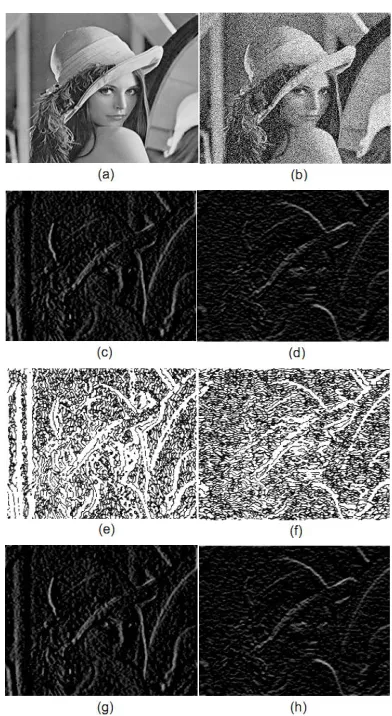
Figure 1 shows
edges are acquired.
the effect of this wavelet transform filtering method at the scale m = 3 and k 3 27
m m
.
In this figure, (a) is the original Lena ima
image containing Gaussian white noise with the standard deviation 35
ge, (b) is noised
. Wc 1
3,n and Wc 2
3,n aregiven in Fi c) ectivel
1
3, gures 1( 1
4, and (d), resp y.Wc n Wc n and
are shown in Figures1 (f). Figures 1(g) and 2
4,n 2 3,Wc n Wc
(e) and (h)
present 1
3,new
W n and
we acquire the fil-te
1 2 3,
new
W n .
By the above mentioned approach, red dyadic wavelet transform data
k1
new m J
W
1,n2 , we can rec
. Let
k
k
kd
on-
2
, ,
new J
W J n W J n W f n
struct the filtered image from the set
1 , , 2 , ,
J
new new 2 1 j J
W j
n W j n S n where
Figure 1. The effect of the new wavelet filtering at the scale
m = 3 and m k m327. (a) The original Lena image; (b) the noised image; (c) W
( ; (h) Wnew 2
3n
1 3,
c n ; (d) Wc 2
3,n ; (e) 1
1
3, 4,Wc n Wc n ;
3,n W ; (g)
, .
f) Wc 2 c2
4,n
1 3,
new
th ugh the inverse dyadic wav- elet transform. The fil
Transform Filtering Algorithm for
the discrete wavelet transform of no
1 2 2
1 1
, j ,
k
k d
j J j
W j n W f n n
1 2
2J 2J ,
S n Sd f n n ro
J
and
1 2
2J 2J ,
d
S n S f n n
tering algorithm is summarized as follows.
Wavelet Step 2. Initialize:
,
,
k k k
Wb m n Wc m n W m n, ,
Image Denoising
Step 1. Compute k
,
N N
Filter m n O
k k
,
ised image f x x
1, 2
and its the lower-frequency sm-oothed image: Cr2
m n,
Wc
m n Wc,
k
m1,n
,1 m J 1 for iteration{
Loop for the scale m Step 3. Loop
1 m J 1
{
2 1 2,
max 2 ,
k k
n n n N
Mcr m Cr m n
k
k
,
, 2 k
,
k
Mwc m Wc m where Cr m Mcr m
Loop for each pixel point n
n n1, 2
{
2 k k
Cr b , 2 , k k k
m
m n Cr m n Mwc Mcr m
end loop n }
Loop for each pixel point n
n1,n2
{If
2 k , k ,
Cr b m n Wc m n
0
e m for the pixel
2k ,
Cr m n
k
,
0Wc m n
k
Filter m n, 1
end if
}end loop n
}end loop m }end iteration Scale space filtering: Loop for the scal
{
Loop n
n n1, 2
{ k
,velet coefficient at the maxi-m
, ,
k k
new
W m n Filter m n Wb
m n
}
end loop n }
end loop m Step 4. Compute the wa um scale J:
k
,
k
,
newW J n W J n
Step 5. Reconstruct the image from ed wavelet da
filter ta
k
1
,
new
j J
W j n
and S2J
nThe reconstruction from the set
k
2 1
, , J
new j J
W j n S n
through the inverse dyadic
wavelet transform will yi
inverse dyadic wavelet transform that we implemented in our technique uses a trous algorithm and the quadratic spline scaling functions and wavelets given in [18].
Now we give some comments on the choice of the number of iterations and weight parameter m k . We can design wavelet filtering iteration times and parameter
k m
according to the user’s request. For th umber of iterations, when it is too small, we can not obtain a
oth estimate. If the number of iterations is too large, most of the edge information of reconstructed image will
e n
be eliminated. Thus we should choose a tradeoff between the number of iterations and the estimation of filtered image. It is well known that the Lipschitz exponents of image and noise are different. At the finer scales such as
1
2 and 22, the modulus maxima mainly produced by noise, while at coarser scale, most modulus maxima duced image. So if we set the different value of
k m
pro by
at the different scale m, noise will be eliminated more effectively. In general, let parameter k
m
be lager e larger scale.
4. Experimental Results
at th
We use Peak-Signal-Noise-Ratio Square-Error (RMSE) to evalua
(PSNR) and Root-Mean- te restored results. PSNR and RMSE is defined by the following:
2
255 , 10 log10
1
PSNR u w
2 , , , i j i j i j
u w
mn
(14)
2, ,
,
1
, i j i j i j
RMSE u w u w
mn
, (15)where and denotes the pixel valu
processed and the original images respectively. Hard- ldin sof
entioned Lena im- ag
presses more noise while preserves m
sian noise with the standard de
,
i j
w ui j, es of the
thresho g and t-thresholding are widely used for denoising in image processing by many researchers. Therefore, in the following tests the hard-thresholding method, soft-thresholding method, Xu’s method and Zheng’s method will be used to compare with the dyadic wavelet transform filtering algorithm.
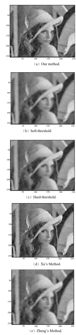
Example 1:When we use our filtering method to do
denoising experiment for the above m
e corrupted by additive noise, the restored result is Figure 2(a). If apply softthreshold, hard-threshold, Xu’s method and Zheng’s method to filter the noised image, the result is in Figures 2(b)-(e).
Table 1 presents the values of PSNR and RMSE for each of the schemes.
From all the five restored images, it is clear that our proposed method sup
ore fine details and small structures in the image. In addition, from the values of PSNR and RMSE for res- tored image, our method increases the PSNR by 1 - 3 dB and reduce the RMSE 5 - 6.
Example 2: A texture image is used in the second test. It is added by the white Gaus
viation 30. Use our filtering method, soft-thr- esholding method, hard-thresholding method, Xu’s met- hod and Z method to process noised image, we can find that our method is also better than other four methods. Figure 3(a) is the original image, Figure 3(b) is the noised image. Figures 4(a)-(e) show the results
50
100
200 150
250
250 200 150 100 50
(a)Our method.
50
100
200 150
250
250 200 150 100 50
(b)Soft-threshold
50
100
200 150
250
250 200 150 100 50
(c)Hard-threshold.
50
100
200 150
250
250 200 150 100 50
(d)Xu’s Method.
50
100
200 150
250
250 200 150 100 50
(e)Zheng’s Method.
heng’s
[image:5.595.352.485.81.661.2]processed by the five methods.
[image:5.595.80.288.272.344.2]Figure 2. Filtered results. (a) Our method; (b) Soft-threshold; (c) Hard-threshold; (d) Xu’s method; (e) Zheng’s method.
Table 1. PSNR and RMSE for each of the schemes.
threshold method method Method method Our threshold Soft- Hard- Xu’s Zheng’s
PSNR 25.2035 dB 23.1125 dB 22.4597 dB 24.0583 dB23.1079 dB RMSE 14.0076 17.8203 19.2111 15.9818 17.8297
50
100
200 150
250
250 200 150 100 50
(a)Original image.
50
100
200 150
250
250 200 150 100 50
[image:6.595.313.536.236.335.2](b)Noised image.
Figure 3. Texture image. (a) Original image; (b) Noised image.
50
100
200 150
250
25 200 150 100 50
(a)Our method.
0 50
100
200 150
250
250 200 150 100 50
(b)Soft-threshold.
50
100
200 150
250
250 200 150 100 50
(c)Hard-threshold.
50
100
200 150
250
250 200 150 100 50
(d)Xu’s Method.
50
100
200 150
250
250 200 150 100 50
(e)Zheng’s Method.
Figure 4. Results for the texture image. (a) Our method; (b) Soft-threshold; (c) Hard-threshold; (d) Xu’s method; (e) Zheng’s method.
[image:6.595.59.284.294.618.2]od Soft-threshold Hard-threshold method Xu’s Zheng’s method Table 2. PSNR and RMSE for restored images.
Method Our meth
PSNR 24.1536 dB 22.5607 dB 22.5533 dB 22.3974 dB 22.7774 dB
From t s ot
visual ti r pr
he results above, it is obviou that n only for quality of images, but
ualso for quantitative evalua-r d on of
ocessing is still better than other four methods. estored ages, o metho im in tex re im e tu ag
Example 3: We use a man image containing both a
human face and some textures to do the third test. The challenge with this image is to keep both texture details and smooth transitions in the human face in the process-ing. We add the original image (Figure 5(a)) with the white Gaussian noise with σ = 30, and get a noised image (Figure 5(b)). Figures 6(a)-(e) are the results obtained by five methods
50 50
100
200 150
250
250 200 150 100 50
(a)Original image. 100
200 150
250
250 200 150 100 50
(b)Noisy image.
Figure 5. Man image. (a) Original image; (b) Noisy image.
50
100
200 150
250
25 200 150 100 50
(a)Our method. 0
50
100
200 150
250
250 200 150 100 50
(b)Soft-threshold
50
100
200 150
250
250 200 150 100 50
(c)Hard-threshold.
50
100
200 150
250
250 200 150 100 50
(d)Xu’s Method.
50
100
200 150
250
250 200 150 100 50
[image:6.595.312.536.364.684.2](e)Zheng’s Method.
Figure 6. Results for man image. (a) Our method; (b) Soft- threshold; (c) Hard-theshold; (d) Xu’s method; (e) Zheng’s method.
[image:6.595.55.289.680.722.2]Table 3 is the quantitative comparison among the five methods.
The results above reveal that our method not only maintain more texture details and smooth transitions in the face but also suppress more noise than other methods after processing. Additionally, our method can increase more PSNR and decrease RESE than other methods.
At last, we give some other types of images. And we only present results recovered by our m thod. A MR
w
aintain all important information and filter out m
wavelet transform filtering
method method e
image (see Figure 7(a)) has been corrupted with white Gaussian noise (σ = 20) and become a noised image, see Figure 7(b). After the noised image has been processed ith our method, we can see that our restoration scheme is able to m
uch noise, see Figure 7(c).
Figures 8(a), (b) and (c) are an original building im-age, the noised imim-age, and the processed result by our method. We can see that the recovered image can pre-serve more image edge details.
A fingerprint image is used in the last test. Figures 9(a)-(c) are the original image, the noised image with σ = 15, and the recovered result with our scheme. From the visual quality, it is obvious that restored image is as good as the original one.
5. Conclusions
[image:7.595.57.289.423.695.2]We have introduced the dyadic
Table 3. Comparison of PSNR and RMSE for restored images.
Method method Our Soft-threshold Hard-threshold Xu’s Zheng’s
PSNR 25.7523 dB 23.8359 dB 23.5585 dB 24.4842 dB 23.7759 dB RMSE 13.1500 16.3963 16.9284 15.2171 16.5099
50
100
200 150
250
50 150 200 250
ginal image.
100 (a)Ori
50
100
200 150
250
100 50
(b)Noised
250 200 = 20. 150 image with σ
50
100
200 150
250
250 200 150 100 50
(c)The result recovered with our scheme.
50
100
200 150
250
250 200 150 100 50
(a)Original image.
50
100
200 150
250
250 200 150 100 50
(b)Noised image with σ = 30.
50
100
200 150
250
250 200 150 100 50
im-age with σ = 30; (c) The result recovered with our scheme.
(c)The result recovered with our scheme.
Figure 8. Building image. (a) Original image; (b) Noisy
50
100
200 150
250
250 200 150 100 50
(a)Original image.
50
100
200 150
250
250 200 150 100 50
(b)Noised image with σ = 15.
50
100
200 150
250
250 200 150 100 50
(c)The result recovered with our scheme.
Figure 9. Fingerprint image. (a) Original image; (b) Noised image with σ = 15; (c) The result recovered with our scheme.
technique for denoising in image processing. Our filtering algorithm is superior to soft-thresholding method, hard- thresholding method, Xu’s method and Zheng’s method because important edge features in the wavelet transform domain are preserved while much noise is suppressed. The other filtering methods perform very poorly in image denoising because they tends to remove the high-fre- quency component exclusively, which yields smooth im- ages and blurs the image edge features.
6. Acknowledgements
This work was supported by the Key Project of Ch Ministry of education (No. 109030), 382 Training Pr amme of CUC(G08382316), and Science Research Pro-ject of Communication University of China(XNL1003). The authors would like to thank the reviewers for ve useful comments, which improved the manuscript sig-nificantly.
tiscale Edges,” IEEE Transactions on Pattern Analy-inese
ogr-
ry
REFERENCES
[1] S. Mallat and S. Zhong, “Characterization of Signal from Mul
sis and Machine Intelligence, Vol. 14, No. 7, 1992, pp. 710-732. doi:10.1109/34.142909
[2] S. Mallat and W. L. Hwang, “Singularity Detection and Processing with Wavelets,” IEEE Transactions on Infor-mation Theory, Vol. 38, No. 2, 1992, pp. 617-643.
doi:10.1109/18.119727
[3] J. L. Starck and A. Bijaoui, Filtering and Deconvolution by the Wavelet Transform,” Signal Processing, Vol. 35, No. 3, 1994, pp. 195-211.
doi:10.1016/0165-1684(94)90211-9
[4] A. Bijaoui, “Wavelets, Ga Signal Processing, Vol. 82
ussian and Wiener Filter , No. 4, 2002, pp. 709-712.
ing,”
doi:10.1016/S0165-1684(02)00137-8
[5] P. L. Shui, “Image Denoising Algorithm via Best Wavelet Packet Base Using Wiener Cost Function,” Institution of Engineering and Technology Image Processing, Vol. 1, No. 3, 2007, pp. 311-318.
[6] Y. Xu, J. B. Weaver, et al., “Wavelet Transform Domain Filters: A Spatially Selective Noise Filtration Technique,” IEEE Transactions on Image Processing, Vol. 3, No. 6, 1994, pp. 747-758.
[7] C. Okechukw ctive Noise
Filtra-Image Denois
eucom.2008.04.016
u and C. Ugweje, “Sele
tion of Image Signals Using Wavelet Transform,” Imag-ing Measurement Systems, Vol. 36, No. 3-4, 2004, pp. 279-287.
[8] M. Nasri and H. Nezamabadi-pour, “ ing in the Wavelet Domain Using a New Adaptive Thresholding
Function,” Neurocomputing, Vol. 72, No. 4-6, 2009, pp. 1012-1025. doi:10.1016/j.n
8, 2000, pp. 1535-1549.
[9] Y. Zheng, D. B. H. Tay, et al., “Signal Extraction and Power Spectrum Estimation Using Wavelet Transform Scale Space Filtering and Bayes Shrinkage,” Signal Proc-essing, Vol. 80, No.
doi:10.1016/S0165-1684(00)00054-2
[10] Y. Leung, J. S. Zhang and Z. B. Xu, “Clustering by Scale-Space Filtering,” IEEE Transaction on Pattern An- alysis and Machine Intelligence, Vol. 22, No. 12, 2000,
, pp. 446- pp. 1396-1410.
[11] J. Kalif, S. Mallat and B. Rouge, “Deonvolution by Thresholding in Mirror Wavelet Bases,” IEEE Transac-tion on Image Processing, Vol. 12, No. 4, 2003
457. doi:10.1109/TIP.2003.810592
[12] Y. F. Zheng and R. L. Ewing, “Feature-Based Wavelet Shrinkage Algorithm for Image Denoising,” IEEE Trans-action on Image Processing, Vol. 14, No. 1
2024-2039.
2, 2005, pp.
y and Machine, Vol. 37, No. 4, 2007, pp. [13] Z. Y. Chen, X. P. Guo, X. L. Zhang, W. J. Cram and Z. W. Li, “A Novel Method for Analysis of Single Ion Channel Signal Based on Wavelet Transform,” Com-puters in Biolog
559-562. doi:10.1016/j.compbiomed.2006.08.006
[14] D. L. Donoho and I. M. Johnstone, “Ideal Spatial Adap-tion via Wavelet Shrinkage,” Biometrika, Vol. 81, No. 3, 1994, pp. 425-435. doi:10.1093/biomet/81.3.425
[15] D. L. Donoho, “De-Noising by Soft-Thresholding,” IEEE Transaction on Information Theory, Vol. 41, No. 3, 1995, pp. 613-627. doi:10.1109/18.382009
[16] M. Holschneider, R. Kronland-Martinet, J. Morlet and P.
of 8th Tchamitchian, “Wavelets, Time-Frequency Methods and Phase Space, Chapter A Real-Time Algorithm for Signal Analysis with the Help of the Wavelet Transform,” Springer-Verlag, Berlin, 1989, pp. 289-297.
[17] A. Witkin, “Scale Space Filtering,” Proceedings International Joint Conference on Artificial Intelligence, Karlsruhe, 1983, pp. 1019-1022.