Accelerating Sparse Matrix Operations in Neural Networks on Graphics Processing Units

6215

Accelerating Sparse Matrix Operations in Neural Networks

on Graphics Processing Units

Arturo Argueta and David Chiang Department of Computer Science and Engineering

University of Notre Dame

{aargueta,dchiang}@nd.edu

Abstract

Graphics Processing Units (GPUs) are com-monly used to train and evaluate neural net-works efficiently. While previous work in deep learning has focused on accelerating opera-tions on dense matrices/tensors on GPUs, ef-forts have concentrated on operations involv-ing sparse data structures. Operations usinvolv-ing sparse structures are common in natural lan-guage models at the input and output layers, because these models operate on sequences over discrete alphabets. We present two new GPU algorithms: one at the input layer, for multiplying a matrix by a few-hot vector (gen-eralizing the more common operation of mul-tiplication by a one-hot vector) and one at the output layer, for a fused softmax and top-N se-lection (commonly used in beam search). Our methods achieve speedups over state-of-the-art parallel GPU baselines of up to 7× and 50×, respectively. We also illustrate how our methods scale on different GPU architectures.

1 Introduction

The speedups introduced by parallel architectures inspired the development of accelerators tailored towards specialized functions. Graphics Process-ing Units (GPUs) are now a standard platform for deep learning. GPUs provide faster model training and inference times compared to serial processors, because they can parallelize the linear algebra op-erations used so heavily in neural networks (Raina et al.,2009).

Currently, major open source toolkits (Abadi et al., 2016) provide additional layers of abstrac-tion to support one or more parallel GPU architec-tures. The seamless compatibility with multiple GPUs allows researchers to train a single model on multiple hardware platforms with no signifi-cant changes to their code base and no specialized knowledge about the targeted architectures. The

disadvantage of hardware agnostic APIs is the lack of optimizations for a set of task-specific func-tions.

Adapting parallel neural operations to a spe-cific hardware platform is required to obtain op-timal speed. Since matrix operations are used heavily in deep learning, much research has been done on optimizing them on GPUs (Chetlur et al.,

2014;Gupta et al.,2015). Recently, some efforts have been made to other kinds of operations: se-rial operations running on the GPU (Povey et al.,

2016), operations not involving matrix multiplica-tions (Bogoychev et al.,2018), and models using sparse structures (Zhang et al.,2016). In this pa-per, we focus on sparse operations running exclu-sively on the GPU architecture.

Much recent work in High Performance Com-puting (HPC) and Natural Language Processing (NLP) focuses on an expensive step of a model or models and optimizes it for a specific architecture. The lookup operation used in the input layer and the softmax function used in the output are two examples seen in machine translation, language modeling, and other tasks. Previous work has ac-celerated the softmax step by skipping it entirely (Devlin et al., 2014), or approximating it (Shim et al.,2017;Grave et al.,2017).

Another strategy is to fuse multiple tasks into a single step. This approach increases the room for parallelism. Recent efforts have fused the softmax and top-Noperations to accelerate beam search on the GPU using similar approaches (Hoang et al.,

for GPUs.

NMT uses beam search during inference to limit the full set of potential output translations ex-plored during decoding (Cho et al.,2014;Graves,

2012). This algorithm is widely used to obtain state-of-the-art results during test time. At each decoding time-step t, the top-N hypotheses are chosen for further expansion and the rest are dis-carded. The top-N selection part of the search has been accelerated using hashing methods to avoid a full sort (Shi et al.,2018;Pagh and Rodler,2004). The aim of this paper is to both combine softmax and top-N operations seen in the last layer of a neural network and optimize the top-N selection operation used by several NMT models.

Our work uses ideas from previous work to ac-celerate two different operations. We focus on op-erations that manipulate sparse structures (Saad,

1990). By sparse, we mean operations that only require a small fraction of the elements in a tensor to output the correct result. We propose two dif-ferent optimizations for sparse scenarios in deep learning: The first operation involves the first layer of a neural network. We accelerate the first matrix multiplication using batched sparse vectors as in-put. The second operation is the computation of the softmax used for beam search. We combine the softmax and the top-N selection into one op-eration obtaining a speedup over a parallel state-of-the-art baseline. We show that our fused

top-N selection and sparse lookups achieve speedups of 7× and 50× relative to other parallel NVIDIA baselines.

2 Graphics Processing Units

GPUs are widely used to accelerate a variety of non-neural tasks such as search (Garcia et al.,

2008), parsing (Hall et al.,2014), and sorting ( Sin-torn and Assarsson,2008). Applications adapted to the GPU spot different architectural properties of the graphics card to obtain the best perfor-mance. This section provides a short overview of the architectural features targeted for this work.

2.1 CUDA execution model

CPUs call special functions, also called kernels, to execute a set of instructions in parallel using multiple threads on the GPU. Kernels can be con-figured to create and execute an arbitrary number of threads. The threads in a kernel are grouped into different thread blocks (also called

cooper-ative thread arrays). Threads in the same block can collaborate by sharing the same memory cache or similar operations. The maximum number of threads per block and number of blocks varies across GPU architectures.

All threads running in the same block are as-signed to a single Streaming Multiprocessor (SM) on the GPU. A SM contains the CUDA cores that execute the instructions for each thread in a sin-gle block. The number of CUDA cores per SM varies depending on the architecture. For exam-ple, Volta V100 contain 64 cores per SM, while GeForce GTX 1080s contain 128 cores per SM. Multiple thread blocks can be assigned to a SM if the number of blocks in the grid is larger than the number of physical SMs. Execution time will in-crease when more than one block is assigned to all SMs on the device (assuming all blocks run the same instruction). Regardless of the number of threads per block, all SMs can only run a to-tal of 32 threads, called a warp, asynchronously at a time. Warp schedulers select in a round-robin fashion a warp from an assigned block to exe-cute in parallel. The SMs finish execution when all blocks assigned to them complete their tasks. Each thread running on the SM can access multi-ple levels of memory on the graphics card, and an efficient use of all levels significantly improves the overall execution time on the device.

2.2 Memory

main use of this memory is to store all the data copied from and to the host CPU. The amount of global memory varies depending on the GPU model (e.g. 12GB on the K40 and 16GB on the V100).

An efficient use of the memory hierarchy pro-vides the best performance. A parallel application must be designed to minimize the total amount of calls to global memory while maximizing the use of registers and shared memory. An exclusive use of main memory will produce the worst execution times. Our methods focus on the efficient use of shared and register memory for scenarios where the data is small enough to fit.

2.3 GPU Sorting

Currently, state-of-the-art methods use a tree-based reduction operation (Harris, 2005) to sort the list on the GPU and obtain the top elements. Reductions are most efficient when the input needs to be completely sorted, yet faster algorithms can be used if only a portion of the sorted output is needed.

The top-Noperation can be accelerated with an improved sorting algorithm for the beam search task on the GPU. Beam search only requires the top-Nentries for each mini-batch, and the entries do not need to be sorted in a specific order (as-cending or des(as-cending). Storing the irrelevant el-ements for beam search back into global memory is not required for this task and should be avoided. A clear optimization is to obtain the top elements in each minibatch using a faster sorting algorithm. Distinct sorting algorithms can be used to ob-tain the top elements from a set of candidates. Pre-vious work introduced custom sorting algorithms for specific tasks using multi-core CPU (Tridgell,

1999) and GPU setups (Satish et al.,2009; Govin-daraju et al.,2006).

3 Background

In this section, we describe two sparse operations commonly used in deep learning, especially for NLP: at the input layer, multiplication by a sparse matrix, and at the output layer, softmax and selec-tion of the top-Nelements.

3.1 N-hot lookup

In models whose inputs are words, the input layer typically looks up a learned word embedding for each word. Equivalently, it represents each word

as a one-hot vector (whose dimensionality is equal to the vocabulary size, K) and multiplies it (as a row vector) by aK×MmatrixBwhose rows are word embeddings. Then, a minibatch ofLwords can be represented as aL×KmatrixAwhose rows are one-hot vectors, so that the productC= ABis a matrix whose rows are the embeddings of the words in the minibatch. Deep learning toolkits (Neubig et al.,2017;Jia et al., 2014) do not per-form a full matrix multiplication; typically, they implement a specialized operation to do this.

A problem arises, however, when the input vec-tor is not a one-hot vecvec-tor, but an “N-hot” vec-tor. For example, we might use additional dimen-sions of the vector to represent subword or part-of-speech tag information (Niehues et al., 2011;

Collobert et al.,2011;Chiu and Nichols,2016). In this case, it would be appropriate to use a sparse matrix library like cuSPARSE, but we show below that we can do better.

3.2 Softmax

The softmax function (Equation1) is widely used in deep learning to output a categorical probability distribution:

softmax(z)j =

exp(zj) P

j0exp(z_j0) (1)

For better numerical stability, all deep learning toolkits actually compute the softmax as follows:

softmax(z)j =

exp(zj−max(z)) P

j0exp(z_j0−max(z)) (2)

This alternative requires different optimizations on the GPU given the max operation. Recent work (Milakov and Gimelshein,2018) explore different techniques to calculate this safe softmax version efficiently.

3.3 Beam search and top-Nselection

Some applications in deep learning require ad-ditional computations after the softmax function. During NMT decoding, the top-N probabilities from softmax(z) are chosen at every time-step t

Algorithm 1Serial minibatched softmax and

top-Nalgorithm.

InputC∈_RL×K OutputD∈_RL×N

1: for`←1, . . . ,Ldo

2: d` ←0

3: fork←1, . . . ,Kdo

4: for`←1, . . . ,Ldo

5: d`+=exp(C[`][k])

6: fork←1, . . . ,Kdo .softmax

7: for`←1, . . . ,Ldo

8: C[`][k]←exp(C[`][k])/d`

9: for`←1, . . .Ldo .top-N

10: c←sort(C[`])

11: D[`]←c[1 :N]

12: returnD

retrieval of non-zero elements in a sparse input parallels the top-Nscenario. (Beam search also re-quires that we keep track of the original column in-dices (i.e., the word IDs) of the selected columns; this is not shown in Algorithm1for simplicity.)

In NMT, the top-N operation consumes a sig-nificant fraction of time during decoding. Hoang et al.(2018) find that the softmax operation takes 5% of total decoding time, whereas finding the top-N elements can take up to 36.8%. So there is a large potential benefit from speeding up this step.

4 Method

In this section, we present our algorithms for N -hot lookup (§4.1) and fused softmax and top-N se-lection (§4.2).

4.1 Sparse input lookups

Our sparse N-hot lookup method, shown in Al-gorithm 2, multiplies a sparse matrix A in Com-pressed Sparse Row (CSR) format by a row-major matrixBto yield a dense matrixC.

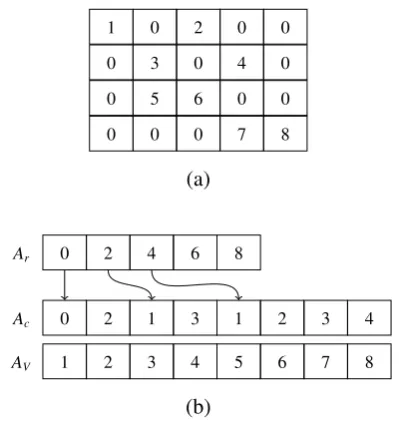
CSR is widely used to store and process sparse matrices. This format stores all non-zero elements of a sparse matrixAcontiguously into a new struc-ture Av. Two additional vectorsAr andAcare

re-quired to access the values in Av. An example of

the CSR format is illustrated in Figure1.Aris first

used to access the columns storing the non-zero el-ements in row`. The number of non-zero elements for a row ` can be computed by accessing Ar[`]

and calculating its offset with the next element

1 0 2 0 0

0 3 0 4 0

0 5 6 0 0

0 0 0 7 8

(a)

Ar 0 2 4 6 8

Ac 0 2 1 3 1 2 3 4

AV 1 2 3 4 5 6 7 8

(b)

Figure 1: Example CSR representation for a sparse ma-trix (a). The CSR representation (b) relies on three lists R, C, and V to store a sparse matrix. Rrepresents the rows,Cthe columns, andVstores the non-zero values.

Ar[`+1].Ar[`] is also used to index the lists

con-taining the columns (Ac) and corresponding

non-zero values (Av) in rowA[`]. For example, to

cal-culate the number of non-zero values in the second row of Figure 1, The offset Ar[3]−Ar[2] = 2 is

calculated. Finally,Ar[2] points to positions 4 and

5 on AcandAv storing the columns and non-zero

values for that specific row.

Our method computes the matrix multiplication by processing the elements of the output matrixC

in parallel. For our experiments, we process 32 (warp size) rows and columns in parallel for the input matrices. We cannot use a stride size larger than 32, since certain GPU architectures do not al-low a 2 dimensional block larger than 32×32 (or a block containing more than 1024 threads total). Although this method is fairly straightforward, we will see below that it outperforms other methods whenNis small, as we expect it to be.

4.2 Fused softmax and top-N

in-Algorithm 2 Sparse matrix multiplication using the CSR format.

InputAr∈RL,Ac ∈RLN,Av∈RLN,B∈RK×M

OutputC∈_RL×M

1: parform←1, . . . ,Mdo .Block level

2: parfor`←1, . . . ,Ldo .Block level

3: x←0

4: kstart ←Ar[m]

5: kend ←Ar[m+1]

6: fork←kstart, . . . ,kend−1do

7: z←Ac[k]

8: y←Av[k]

9: x+=y×B[z][`]

10: C[`][m]←x

11: returnC

Algorithm 3Top-N selection based on insertion sort.

InputarrayC ∈_RK OutputarrayD∈_RN

1: forn←1, . . . ,Ndo

2: D[n]← −∞

3: fork←1, . . .Kdo

4: forn←1, . . . ,Ndo

5: ifC[k]>D[n]then

6: swapD[n] andC[k]

sertion sort, it maintains separate buffers for the sorted portion (D) and the unsorted portion (C); it also performs an insertion by repeating swapping instead of shifting.

The key to our method is that we can paral-lelize the loop over k (line 3) while maintaining correctness, as long as the comparison and swap can be done atomically. To see this, note that no swap can ever decrease the value of one of the

D[n]. Furthermore, because for eachk, we com-pareC[k] with every element ofD, it must be the case that after looping over alln(line4), we have

C[k] ≤ D[n] for alln. Therefore, when the algo-rithm finishes,Dcontains the top-Nvalues.

Fusing this algorithm with the softmax algo-rithm, we obtain Algorithm 4. It takes an in-put array C containing a minibatch of logits and returns an array D with the top-N probabilities and an array E with their original indices. The comparisons in our method are carried out by the CUDAatomicMaxoperation (line12). This func-tion reads a valueD0[`][n] and computes the

max-Algorithm 4Parallel fused batched softmax, and top-N algorithm. The comment “kernel-level” means a loop over blocks, and the comment “block-level” means a loop over threads in a block.

InputC∈_RL×K

OutputD∈_RL×N,E ∈ {1, . . . ,K}L×N

1: parfor`←1, . . . ,Ldo .kernel-level

2: d` ←0

3: e` ← −∞

4: forn←1, . . .Ndo

5: D0[`][n]←pack(−∞,0)

6: parfor`←1, . . . ,Ldo .kernel-level

7: parfork←1, . . . ,Kdo .block-level

8: x←C[`][k]

9: y←pack(x,k)

10: e`←atomicMax(C[`][k],e`)

11: forn←1, . . . ,Ndo

12: c0 ←atomicMax(D0[`][n],y)

13: ifc0 <ythen

14: y←c0

15: syncthreads()

16: d`+=exp(C[`][k]−e`)

17: syncthreads()

18: forn←1, . . . ,Ndo

19: x,i←unpack(D0[`][n])

20: D[`][n]←exp(x)/d`

21: E[`][n]←i

22: returnD

imum between it and a second valuey. The larger is stored back intoD0[`][n], and the original value ofD0[`][n] is returned asc0. This operation is per-formed as one atomic transaction. The following two lines (13-14) sety to the smaller of the two values.

Our algorithm recovers the original column in-dices (m) with a simple extension following Ar-gueta and Chiang(2017). We pack each probabil-ity as well as its original column index into a sin-gle 64-bit integer before the sorting step (line 5), with the probability in the upper 32 bits and the column index in the lower 32 bits. This represen-tation preserves the ordering of probabilities, so a singleatomicMaxoperation on the packed repre-sentation will atomically update both the probabil-ity and the index.

ker-(a) Tesla V100

Method Number of dense values (N)

1 2 3 4 5 10 50 100

ours 0.02 0.02 0.02 0.02 0.02 0.03 0.06 0.11

cuBLAS 0.16 0.16 0.16 0.16 0.16 0.16 0.15 0.15 cuSPARSE 0.15 0.16 0.16 0.16 0.16 0.17 0.16 0.19

(b) TITAN X

Method Number of dense values (N)

1 2 3 4 5 10 50 100

ours 0.03 0.04 0.05 0.07 0.08 0.14 0.49 0.90 cuBLAS 1.79 1.63 1.68 1.68 1.70 1.57 1.27 0.86 cuSPARSE 0.12 0.12 0.12 0.12 0.13 0.13 0.16 0.21

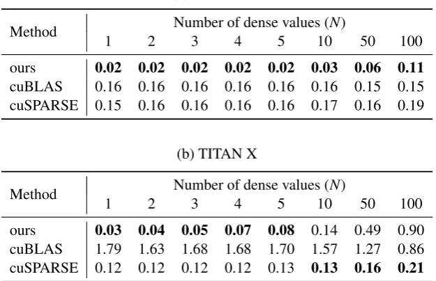
Table 1: Performance comparison for theN-hot lookups against the NVIDIA baseline using dimensionsL=100, K=10240,N=512. Each time (in ms) is an average over ten runs. Fastest times are in bold.

nel and memory configurations to obtain the best performance. The number of kernel blocks must be equal to the number of elements in the mini-batch. This means that batch sizes smaller than or equal to the number of SMs on the GPU will run more efficiently given only one block, or less, will run on all SMs in parallel. The overall perfor-mance will be affected if multiple blocks are as-signed to all SMs. The number of SMs on the GPU varies depending on the architecture. For exam-ple, the Tesla V100 GPU contains 80 SMs, while the Pascal TITAN X contains 30 SMs. This means that our method will perform better on newer GPU architectures with a large amount of SMs. The number of threads in the block is an additional as-pect to consider for our method.

The block size used for our experiments is fixed to 256 for all the experiments. This number can be adapted if the expected number of hypotheses to sort is smaller than 256 (the number of threads must be divisible by 32). The amount of shared memory allocated per block depends on the size ofN. The auxiliary memory used to store the

top-N elements must fit in shared memory to obtain the best performance. A largeNwill use a combi-nation of shared and global memory affecting the overall execution of our method.

5 Experiments

We run experiments on two different GPU con-figurations. The first setup is a 16 core In-tel(R) Xeon(R) Silver 4110 CPU connected to a

Tesla V100 CPU, and the second set is a 16-core Intel(R) Xeon(R) CPU E5-2630 connected to a GeForce GTX TITAN X. The dense matrices we use are randomly generated with different floating point values. We assume the dense representations contain no values equal to zero. The sparse mini-batches used for the top-N experiments are ran-domly generated to contain a specific amount of non-zero values per element. The indices for all non-zero values are selected at random.

5.1 SparseN-hot lookups

For the N-hot lookup task, we compared against the cuBLAS1and cuSPARSE2parallel APIs from NVIDIA. Both interfaces provide methods to compute mathematical operations in parallel on the GPU. Table 1 shows the performance of our method against the two NVIDIA APIs for sparse and dense matrix multiplication using different ar-chitectures and levels of sparsity. All speedups de-crease as the input becomes less sparse. The cuS-PARSE baseline performs on par with the dense cuBLAS version on the V100 architecture when the number of non-zero elements per batch is larger than 1. The cuSPARSE baseline performs better than its dense counterpart on the TITAN X architecture and worse on the V100. An ex-planation behind this is the type of sparsity pat-terns cuSPARSE handles and the different amount of SMs and memory types on both architectures.

a) Tesla V100

Method L Number of top-Nelements

10 20 30 40 50 100 200 300 400

Ours 1 0.07 0.11 0.15 0.19 0.21 0.57 1.54 2.85 4.49 Milakov et al. 1 3.56 3.43 3.44 3.46 3.44 3.44 3.44 3.44 3.44

Speedup 50.85 32.41 23.47 18.01 14.21 6.03 2.23 1.20 0.76 Ours 512 0.14 0.22 0.30 0.39 0.49 1.15 3.03 5.70 9.05 Milakov et al. 512 7.99 8.45 7.98 8.00 8.01 8.01 8.01 8.02 8.02

Speedup 54.79 37.22 25.84 20.03 16.13 6.95 2.64 1.40 0.88

Ours 1024 0.25 0.38 0.54 0.72 0.93 2.37 6.57 12.09 19.65

Milakov et al. 1024 12.54 12.70 12.58 12.58 13.02 12.59 12.62 12.59 12.58

Speedup 50.08 32.78 23.11 17.34 13.88 5.30 1.91 1.04 0.64

b) TITAN X

Method L Number of top-Nelements

10 20 30 40 50 100 200 300 400

Ours 1 0.09 0.14 0.19 0.25 0.32 0.75 2.09 3.97 6.37

Milakov et al. 1 7.65 7.60 7.61 7.64 7.63 7.64 7.58 7.61 7.59 Speedup 84.10 54.19 39.12 29.92 23.76 10.18 3.62 1.91 1.19

Ours 512 0.59 1.03 1.53 2.17 2.96 6.55 18.94 36.20 56.70

Milakov et al. 512 19.23 19.21 19.21 19.22 19.26 19.23 19.02 18.45 18.31

Speedup 32.72 18.64 12.51 8.83 6.48 2.93 1.00 0.50 0.32

Ours 1024 1.07 1.90 2.90 4.13 5.59 12.32 35.22 63.85 101.10

Milakov et al. 1024 31.89 31.91 31.88 31.73 31.91 31.60 30.94 29.55 28.49

Speedup 29.55 16.78 10.97 7.67 5.70 2.56 0.87 0.46 0.28

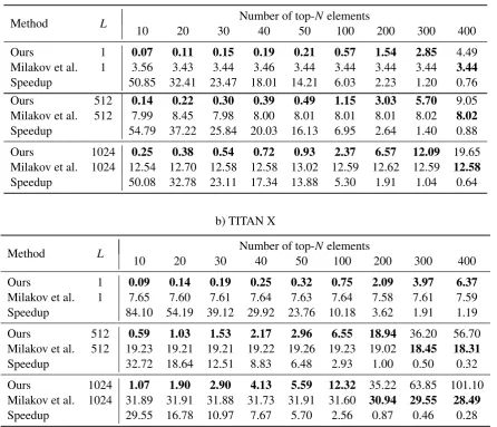
Table 2: Fused softmax and top-Nperformance comparison against the method ofMilakov and Gimelshein(2018) using different values ofNand different batch sizes. For all experiments, we set the vocabulary size toK=10240. Each time (in ms) is an average over ten runs. Fastest times are shown in bold.

cuSPARSE is designed to handle sparsity patterns that translate well on several tasks with different sparsity patterns. The multiplication time remains constant on the V100 when a standard dense ma-trix multiplication is used while cuSPARSE keeps performing worse once the sparse input becomes dense.

The highest speedups are obtained when the amount of non-zero elements is low, and the low-est speedups are seen when the amount of non-zero elements increase. On the V100, our method starts performing worse than the cuBLAS base-line when the amount of non-zero elements per batch element is larger than 100. On the other side, the performance of our method is worse than cuSPARSE when the sparsity is larger than 10 on the TITAN X architecture. Our method performs

well on newer GPU models with a larger amount of SMs.

whereas the other times only include the matrix operation itself.

5.2 Softmax and top-N

We compared our fused softmax operation against the current state-of-the art method from NVIDIA (Milakov and Gimelshein,2018). Table2 demon-strates the comparison of our method against the NVIDIA baseline using two different architec-tures. Our method outperforms the baseline on top-N sizes smaller than or equal to 300. Our method scales differently on both GPU archi-tectures given the constrained amount of shared memory on the graphics cards and the amount of SMs available. The performance of our sug-gested implementation will slightly degrade on both architectures when the amount of memory used to perform the selection overtakes the amount of shared memory available.

The speedups against the baseline decrease as

Ngrows. Our execution time still outperforms the baseline on most sizes ofNused in NMT scenar-ios. This makes our method suitable for tasks re-quiring a small amount of elements from an output list. If the size ofNexceeds 300, different methods should be used to obtain the most optimal perfor-mance.

The baseline scales better than our implemen-tation when N increases. Table 2 shows the ex-ecution time for the baseline is not affected sig-nificantly when N grows. The baseline does see performance degradation when the amount of el-ements in the mini-batch increases. This is due to the same reduction operation used for all sizes of N. This factor allows our method to perform better in several scenarios whereNis smaller than or equal to 300. The baseline performs best on scenarios where the batch size is small and the size of the batch elements is large (about 4000). They claim their method does not perform well on batches with a high dimensionality ifN is very large due to the cost of computing the full reduc-tion to sort the input weights and their ids.

The batch size affects the performance in a dif-ferent manner on both architectures. The per-formance scales in a different manner when the batch size changes. On our largest experiments, the performance for N = 400 does not degrade significantly on the V100 architecture, while the speedups on the TITAN X change significantly from 1.19 to 0.32. This shows that our method

runs best on the TITAN X architecture when the batch size is small, and the amount of top-N el-ements required does not exceed 400. For larger batches, the V100 architecture performs best for all values of N. The TITAN X provides better speedups against the baseline when the number of elements in the mini-batch is small, and both our method and baseline run on the same GPU device.

6 Conclusion

In this work, we introduce two parallel methods for sparse computations found in NMT. The first operation is the sparse multiplication found in the input layer, and the second one is a fused softmax and top-N. Both implementations outperform dif-ferent parallel baselines. We obtained speedups of up to 7×for the sparse affine transformation, and 50×for the fused softmax and top-Ntask.3

Future work includes the fusion of additional operations in neural models. Matrix operations form the largest bottleneck in deep learning. The last affine transformation in deep neural models can be fused with our softmax and top-N meth-ods. The fusion of these three operations requires a different implementation of the matrix multipli-cation, and shared memory usage.

References

Mart´ın Abadi, Paul Barham, Jianmin Chen, Zhifeng Chen, Andy Davis, Jeffrey Dean, Matthieu Devin, Sanjay Ghemawat, Geoffrey Irving, Michael Isard, et al. 2016. Tensorflow: a system for large-scale machine learning. InOSDI, volume 16, pages 265– 283.

Arturo Argueta and David Chiang. 2017. Decoding with finite-state transducers on GPUs. In Proc. EACL, volume 1, pages 1044–1052.

Nikolay Bogoychev, Kenneth Heafield, Alham Fikri Aji, and Marcin Junczys-Dowmunt. 2018. Accel-erating asynchronous stochastic gradient descent for neural machine translation. InProc. EMNLP.

Sharan Chetlur, CliffWoolley, Philippe Vandermersch, Jonathan Cohen, John Tran, Bryan Catanzaro, and Evan Shelhamer. 2014. cuDNN: Efficient primitives for deep learning. arXiv:1410.0759.

Jason Chiu and Eric Nichols. 2016. Named entity recognition with bidirectional LSTM-CNNs. Trans. ACL, 4:357–370.

Kyunghyun Cho, Bart van Merrienboer, Dzmitry Bah-danau, and Yoshua Bengio. 2014. On the properties

of neural machine translation: Encoder-decoder ap-proaches. InProc. Workshop on Syntax, Semantics, and Structure in Statistical Translation.

Ronan Collobert, Jason Weston, L´eon Bottou, Michael Karlen, Koray Kavukcuoglu, and Pavel Kuksa. 2011. Natural language processing (almost) from scratch.J. Mach. Learn. Res., 12:2493–2537.

Jacob Devlin, Rabih Zbib, Zhongqiang Huang, Thomas Lamar, Richard Schwartz, and John Makhoul. 2014. Fast and robust neural network joint models for sta-tistical machine translation. InProc. ACL, volume 1, pages 1370–1380.

Vincent Garcia, Eric Debreuve, and Michel Barlaud. 2008. Fast k nearest neighbor search using GPU. In CVPR Workshop on Computer Vision on GPU, pages 1–6. IEEE.

Naga Govindaraju, Jim Gray, Ritesh Kumar, and Di-nesh Manocha. 2006. GPUTeraSort: High per-formance graphics co-processor sorting for large database management. In Proc. ACM SIGMOD International Conference on Management of Data, pages 325–336.

Edouard Grave, Armand Joulin, Moustapha Ciss´e, David Grangier, and Herv´e J´egou. 2017. Efficient softmax approximation for GPUs. InProc. ICML.

Alex Graves. 2012. Sequence transduction with recur-rent neural networks. InICML Workshop on Repre-sentation Learning.

Suyog Gupta, Ankur Agrawal, Kailash Gopalakrish-nan, and Pritish Narayanan. 2015. Deep learning with limited numerical precision. In Proc. ICML, pages 1737–1746.

David Hall, Taylor Berg-Kirkpatrick, and Dan Klein. 2014. Sparser, better, faster GPU parsing. InProc. ACL, pages 208–217.

Mark Harris. 2005. Mapping computational concepts to GPUs. In ACM SIGGRAPH 2005 Courses, page 50.

Hieu Hoang, Tomasz Dwojak, Rihards Krislauks, Daniel Torregrosa, and Kenneth Heafield. 2018.

Fast neural machine translation implementation. In Proceedings of the 2nd Workshop on Neural Ma-chine Translation and Generation, pages 116–121. Association for Computational Linguistics.

Yangqing Jia, Evan Shelhamer, JeffDonahue, Sergey Karayev, Jonathan Long, Ross Girshick, Sergio Guadarrama, and Trevor Darrell. 2014. Caffe: Con-volutional architecture for fast feature embedding. In Proc. ACM International Conference on Multi-media, pages 675–678.

Philipp Koehn and Rebecca Knowles. 2017. Six chal-lenges for neural machine translation. In Proc. Workshop on Neural Machine Translation, pages 28–39.

Maxim Milakov and Natalia Gimelshein. 2018.

Online normalizer calculation for softmax. arXiv:1805.02867.

Graham Neubig, Chris Dyer, Yoav Goldberg, Austin Matthews, Waleed Ammar, Antonios Anastasopou-los, Miguel Ballesteros, David Chiang, Daniel Clothiaux, Trevor Cohn, et al. 2017. DyNet: The dynamic neural network toolkit. arXiv:1701.03980.

Jan Niehues, Teresa Herrmann, Stephan Vogel, and Alex Waibel. 2011. Wider context by using bilin-gual language models in machine translation. In Proc. Workshop on Statistical Machine Translation, pages 198–206.

Rasmus Pagh and Flemming Friche Rodler. 2004. Cuckoo hashing. Journal of Algorithms, 51(2):122– 144.

Daniel Povey, Vijayaditya Peddinti, Daniel Galvez, Pe-gah Ghahremani, Vimal Manohar, Xingyu Na, Yim-ing Wang, and Sanjeev Khudanpur. 2016. Purely sequence-trained neural networks for ASR based on lattice-free MMI. InProc. Interspeech, pages 2751– 2755.

Rajat Raina, Anand Madhavan, and Andrew Y Ng. 2009. Large-scale deep unsupervised learning us-ing graphics processors. InProc. ICML, pages 873– 880.

Youcef Saad. 1990. Sparskit: A basic tool kit for sparse matrix computations. RIACS Technical Report.

Nadathur Satish, Mark Harris, and Michael Garland. 2009. Designing efficient sorting algorithms for manycore GPUs. InIEEE Intl. Symposium on Par-allel&Distributed Processing, pages 1–10.

Xing Shi, Shizhen Xu, and Kevin Knight. 2018. Fast locality sensitive hashing for beam search on GPU. arXiv:1806.00588.

Kyuhong Shim, Minjae Lee, Iksoo Choi, Yoonho Boo, and Wonyong Sung. 2017. Svd-softmax: Fast soft-max approximation on large vocabulary neural net-works. InAdvances in Neural Information Process-ing Systems, pages 5463–5473.

Erik Sintorn and Ulf Assarsson. 2008. Fast parallel GPU-sorting using a hybrid algorithm. Journal of Parallel and Distributed Computing, 10(68):1381– 1388.

Ilya Sutskever, Oriol Vinyals, and Quoc V Le. 2014. Sequence to sequence learning with neural net-works. InAdvances in Neural Information Process-ing Systems, pages 3104–3112.