A further look at Modified ML estimation of the panel AR(1) model with fixed effects and arbitrary initial conditions

Munich Personal RePEc Archive

A further look at Modified ML

estimation of the panel AR(1) model

with fixed effects and arbitrary initial

conditions.

Kruiniger, Hugo

Department of Economics and Finance, University of Durham

16 June 2018

Online at

https://mpra.ub.uni-muenchen.de/88623/

A further look at Modi…ed ML estimation of the

panel AR(1) model with …xed e¤ects and arbitrary

initial conditions.

Hugo Kruiniger

Durham University

This version: 16 June 2018

Abstract

In this paper we consider two kinds of generalizations of Lancaster’s (Review of Eco-nomic Studies, 2002) Modi…ed ML estimator (MMLE) for the panel AR(1) model with …xed e¤ects and arbitrary initial conditions and possibly covariates when the time di-mension, T, is …xed. When the autoregressive parameter = 1; the limiting modi…ed pro…le log-likelihood function for this model has a stationary point of in‡ection and is …rst-order underidenti…ed but second-order identi…ed. We show that the generalized MMLEs exist w.p.a.1 and are uniquely de…ned w.p.1. and consistent for any value of

1. When = 1; the rate of convergence of the MMLEs is N1=4_{; where N is the}

cross-sectional dimension of the panel. We then develop an asymptotic theory for GMM estimators when one of the parameters is only second-order identi…ed and use this to derive the limiting distributions of the MMLEs. They are generally asymmetric when

= 1:One kind of generalized MMLE depends on a weight matrixWN and we show that

a suitable choice of WN yields an asymptotically unbiased MMLE. We also show that

Quasi LM tests that are based on the modi…ed pro…le log-likelihood and use its expected rather than observed Hessian, with an additional modi…cation for = 1; and con…dence regions that are based on inverting these tests have correct asymptotic size in a uniform sense when _{j j} 1. Finally, we investigate the …nite sample properties of the MMLEs and the QLM test in a Monte Carlo study.

JEL classi…cation: C11, C13, C23.

Keywords: dynamic panel data, expected Hessian, …xed e¤ects, Generalized Method of Moments (GMM), in‡ection point, Modi…ed Maximum Likelihood, Quasi LM test, second-order identi…cation, singular information matrix, weak moment conditions.

1

Introduction

In this paper we reconsider Modi…ed ML estimation (cf. Neyman and Scott, 1948) of the panel AR(1) model with …xed e¤ects (FE) and arbitrary initial conditions and possibly strictly exogenous covariates, when the time dimension of the panel,T, is …xed.

It is well known that the FE ML estimator for the autoregressive parameter that is equal to the LSDV estimator is inconsistent whenT is …xed, cf. Nickell (1981).1 _{To obtain}

a consistent FE estimator for (or for 0 = ( 2 0)0where 2is the error variance and is

the vector of coe¢cients of the covariates) based on the likelihood function for the model, Lancaster (2002) proposed a Bayesian approach that involves using a reparametrization of the …xed e¤ects, which aims to achieve information orthogonality (but fails to do so when covariates are present), and integrating the new e¤ects from the likelihood function using a uniform prior density. He de…ned his estimator for (or for 0) as a local rather

than a global maximizer of the resulting marginal (or joint) posterior density because this posterior density is improper and has a global maximum at r = 1 for any sample size, cf. Dhaene and Jochmans (2016).2 _{Bun and Carree (2005) took a di¤erent route and}

proposed a bias-corrected LSDV estimator for 0 with the correction based on formulae

for the asymptotic biases of the LSDV estimators for and . However, a version of their estimator is equal to Lancaster’s estimator for 0, cf. Dhaene and Jochmans (2016),

and both of them can be viewed as a Modi…ed ML estimator (MMLE), cf. Alvarez and Arellano (2004). Bun and Carree (2005) also investigated the …nite sample properties of their estimator using various Monte Carlo experiments. They reported non-convergence of their estimator in about 40% of the replications in some experiments where N = 100; T = 6 and = 0:8: The possible non-existence of the MMLE is also related to the fact that the underlying density function is improper. Speci…cally, when = 1; the limiting modi…ed pro…le log-likelihood function of r has a stationary point of in‡ection at r= 1, cf. Ahn and Thomas (2004), so that the modi…ed pro…le log-likelihood function may fail to have a local maximum even asymptotically.

In this paper we discuss two kinds of generalizations of Lancaster’s MMLEs that exist as N increases with probability approaching one (w.p.a.1) for any 1.3 _{The …rst}

type of generalized MMLE minimizes a quadratic form in the modi…ed pro…le score vector subject to a second-order condition for a maximum of the modi…ed pro…le likelihood while

1_{FE estimators only use data in di¤erences and are consistent under minimal assumptions.} 2_{Lancaster discards the global maxima at r= 1and only considers local maxima that are}

stationary points.

the second type minimizes the norm of the modi…ed pro…le score for only, subject to a second-order condition for a maximum. The former MMLE depends on a weight matrix. While Lancaster has only argued thatone of the local maxima of the posterior density is consistent (if one exists at all), we show that when 1the generalized MMLEs are uniquely de…ned w.p.1. and consistent.

Both types of generalized MMLEs will select a local maximum if one exists. In this case the estimators are equivalent irrespective of the choice of the weight matrix. However, if the modi…ed pro…le likelihood function of r has no local maximum on the interval[ 1;₁), then these estimators are still consistent but di¤erent and the …rst type of generalized MMLE depends on the choice of the weight matrix.

Dhaene and Jochmans (2016) have shown that their Adjusted Likelihood estimator for the nonstationary panel AR(1) model, which is a constrained version of our second MMLE, is uniquely de…ned asymptotically. However, they have not demonstrated that their constraints, which depend on the LSDV estimator, guarantee uniqueness of their estimator in …nite samples.

We also derive the limiting distributions of the generalized MMLEs. Similar to the cases of the FEMLE of Hsiao et al. (2002) and the REMLE of Chamberlain (1980) and Anderson and Hsiao (1982), if = 1; is only second-order identi…ed by their objective functions and as a result the rate of convergence of the MMLEs for is N1=4_{, cf. Ahn}

and Thomas (2004) and Kruiniger (2013). Our analysis for = 1 is closely related to Sargan (1983) for instrumental variable and ML estimators and also to Rotnitzky et al. (2000) for MLEs when a parameter is only second-order identi…ed, although there are some important di¤erences. We view the MMLEs as GMM estimators in order to derive their limiting distributions when = 1.4 _{Using an appropriate reparametrization of the}

modi…ed pro…le likelihood, we …nd that if = 1 and the data are i.i.d. and normal, then the limiting distributions of the MMLEs are generally asymmetric unlike those of the RE- and FEMLE and other MLEs for parameters that are only second-order identi…ed. Nonetheless, we show that a suitable choice of the weight matrix for the …rst type of generalized MMLE yields an estimator that is asymptotically unbiased when = 1.

Finally, we discuss inference methods related to the modi…ed pro…le likelihood. Wald

4_{Madsen (2009) considers the limiting distribution of another GMM estimator for a panel}

tests, some versions of (Quasi) LM tests, and (Quasi) LR tests that are used for testing hypotheses involving and are based on the reparametrized modi…ed pro…le likelihood do not uniformly converge to their …xed parameter …rst-order limiting distributions when is close or equal to one, cf. Rotnitzky et al. (2000) and Bottai (2003). As a consequence these tests do not asymptotically have correct size in a uniform sense when j j 1. Similarly to Kruiniger (2016) in the case of (Quasi) LM tests related to the RE- and the FE(Q)MLE, we show that (Q)LM test-statistics that are based on the modi…ed pro…le log-likelihood and use itsexpectedrather thanobserved Hessian, with an additional modi…cation for = 1;and con…dence regions that are based on inverting these tests have correct asymptotic size in a uniform sense when _{j j} 1.

Monte Carlo results show that the QLM tests have correct size and that when the data are i.i.d. and normal and j j<1, the MMLEs for can have a signi…cantly smaller RMSE than the asymptotically e¢cient REMLE in panels as large asT = 9andN = 500. When the data are not i.i.d. and normal, it is generally not possible to rank the Quasi MMLEs, the RE- and the FEQMLE in terms of asymptotic e¢ciency.

Both types of generalized MMLEs are also useful for estimating other models with parameters that may correspond to stationary points of in‡ection of the pro…le likelihood function. Examples of such models are the sample selection model and the stochastic production frontier model for a cross-section of units that are discussed in Lee and Chesher (1986) and models with skew-normal distributions, see e.g. Hallin and Ley (2014).

Dhaene and Jochmans (2016) discuss several alternative approaches to constructing modi…ed (pro…le) objective functions for the nonstationary panel AR(1) model that yield estimators similar to Lancaster’s MMLE. Hahn and Kuersteiner (2002) modi…ed the LSDV estimator to remove bias up to order O(T 1_{): Other FE estimators for dynamic}

panel models include the …rst-di¤erence (FD) instrumental variable estimator of Anderson and Hsiao (1981), the FE GMM estimators of Kruiniger (2001), the Maximum Invariant Likelihood estimator of Moreira (2009), the FDMLE of Kruiniger (2008) and the Panel Fully Aggregated Estimator of Han et al. (2015), which is based on X-di¤erencing. The latter two estimators rely on covariance stationarity of the data when _{j j}<1:

2

The panel AR(1) model

We consider ML-type estimators for the panel AR(1) model with K strictly exogenous covariates xi;t;k; k= 1; :::; K :

yi;t = yi;t 1+x0i;t + i+"i;t with = (1 ) and i = (1 ) i; (1)

for i= 1; :::; N and t= 1; :::; T; wherex0i;t is the t th row of theT K matrix Xi; i is

a …xed e¤ect and "i;t is an error term. We can also allow for time e¤ects in the model.

Let yi = (yi;1 ::: yi;T)0; yi; 1 = (yi;0 ::: yi;T 1)0; "i = ("i;1 ::: "i;T)0 and x0i = T 1 0Xi,

with equal to a T vector of ones. If we letvi = ( 1)yi;0+ i+x0i for i = 1; :::; N;

then the model in (1) can also be written as yi yi;0 = (yi; 1 yi;0 ) +QXi +vi +"i

for i = 1; :::; N, where Q = IT T 1 0 and IT is an identity matrix with dimension T;

cf. Lancaster (2002). We make the following assumption:

Assumption 1 The variable yi;t is generated by (1) with (i) T 2; (ii) 1;

(iii) f("0i; vi;(vech(QXi))0)0gNi=1 is a sequence of i:i:d: random vectors with E(vi) = 0;

V ar(vi) = 2v <1 and E(Xi0QXi) is a …nite and positive de…nite matrix; and

(iv) "i ?(vi;(vech(QXi))0)0; E("i) = 0 and V ar("i) = 2IT <1; i= 1; :::; N.

Thus we assume cross-sectional independence, strict exogeneity of the regressors in …rst-di¤erences, homoskedasticity and no multicollinearity. On the other hand, we allow for ARCH and non-normality of the error terms, the"i;t:

We require that T 2 and 1 for identi…cation. In economics the assumption

1 can reasonably be expected to hold when the covariates are strictly exogenous. We allow for >1, that is, we allow for explosive behaviour of thefyi;tgprocesses. When

>1;the assumption 2

v <1implies that thefyi;tgprocesses must have started a …nite

number of periods ago. The restrictive parametrization i = (1 ) i and = (1 )

prevents the …xed e¤ects and the means of the individual regressors from turning into trends at = 1 and thereby avoids a discontinuity in the data generating process at

= 1. These restrictions are only imposed on the DGP but not in estimation.

We are interested in consistent estimation of the common parameters ; 2 _and

3

Modi…ed ML estimation of the panel AR(1) model

Conditional on yi;0 and Xi; i = 1; :::; N and normalized by N, the Gaussian FE

log-likelihood function for the model in (1) is, up to an additive constant, given by:

T

2 logs

2 1

2s2

1

N

N

X

i=1

(yi ryi; 1 Xib ai )0(yi ryi; 1 Xib ai ): (2)

To obtain a consistent FE estimator for 0 based on (2), Lancaster (2002) proposed a

Bayesian approach that involves using a reparametrization of the …xed e¤ects, which aims to achieve information orthogonality (but fails to do so when covariates are present), and integrating the new e¤ects from the likelihood function using a uniform prior density. He de…nes his estimator for 0 as a local maximum of the joint posterior density. Letting

= (r s2 _b)0_{, his joint posterior log-density for the model in (1), normalized byN, which}

can be interpreted as a (normalized) modi…ed pro…le log-likelihood function, is given by:

elN( ) = elN(r; s2; b) = (T 1) (r)

T 1

2 logs

2 ₍₃₎

1 2s2

1

N

N

X

i=1

(yi ryi; 1 Xib)0Q(yi ryi; 1 Xib);

where (r) = 1

T(T 1)

T 1

X

t=1

(T t)

t r

t_{; (4)}

and the corresponding modi…ed pro…le likelihood equations are given by:

( ) = (T 1) 0(r) + 1

s2

1

N

N

X

i=1

(yi ryi; 1 Xib)0Qyi; 1 = 0; (5)

2( ) =

T 1

2s2 +

1 2s4

1

N

N

X

i=1

(yi ryi; 1 Xib)0Q(yi ryi; 1 Xib) = 0;

( ) = 1

s2

1

N

N

X

i=1

X_i0Q(yi ryi; 1 Xib) = 0:

Note that the joint posterior density is not proper.

LetbLAN denote Lancaster’s estimator for 0 and let N be the set of roots of @_@elN = 0

corresponding to local maxima ofelN on which is an open subset of R R+ RK:Thus

b_{LAN 2 N} unless N is empty, in which case (we will say that) bLAN does not exist.

ensures that bLAN always exists so that one can consider whether bLAN is a consistent

estimator for 0:Note that none of the roots of @ elN

@ = 0 correspond to the global maxima

that can occur at r=1 and, if T is odd, at r= 1:

Lancaster showed that elN( ) converges uniformly in probability to a nonstochastic

di¤erentiable function of ; sayel( ); and that @_@el( )j 0 = 0: Next we derive necessary and

su¢cient conditions for negative de…niteness of the Hessian ofel( ) at 0; viz.:

M H =

0 B @

(T 1) 00( ) tr( 0_{Q )} zqz

2

(T 1) 0_{( )} 2

0

xqz

2

(T 1) 0_{( )} 2

T 1

2 4 0

xqz

2 0

xqx

2

1 C

A; (6)

where zqz =plimN!1N 1PN_i=1ZeiQZei; xqx =plimN!1N 1P_iN₌₁Xi0QXi and xqz =

plimN!1N 1PN_i=1Xi0QZei with Zei ='vi + QXi ;

= ( ) =

0 B B B B B B @

0 : : 0 0 0 1 0 0 0 1 0 0

: 1 0 :

: 1 0 :

T 2 _{: : 1 0}

1 C C C C C C A

and '='( ) =

0 B B B B B B B @

1

2

...

T 2

T 1

1 C C C C C C C A

: (7)

It follows from lemma 4.1 in Dhaene and Jochmans (2016) that ifT = 2 and zqz >0

(so that ₆= 1) or if T > 2 and ₆= 1, then M H is negative de…nite so thatel( ) has a local maximum at 0.5 Kruiniger (2001) had already shown that if = 1and T 2;then

M H is singular. Moreover, Ahn and Thomas (2004) have shown that el( ) actually has a stationary point of in‡ection when = 1 rather than a local maximum. This property is related to the fact that the posterior density is not proper. Later on, in the context of Theorem 1 below, we will show that if = 1; elN may not have any local maximum

on e = [ 1;1) (0;1) RK _{asymptotically, so that}b_{LAN is inconsistent.}6 b_{LAN has} two more drawbacks. Firstly, elN( ) may not have any local maximum in small samples,

in which case bLAN does not exist. This may happen when is close or equal to unity.

Secondly, Lancaster did not rule out that elN( ) and el( ) have multiple local maxima on

and he did not explain how to …nd the consistent estimator if that were the case.

5_{Their lemma 4.1 implies that} 00_{( ) (T 1)} 1_tr( 0_{Q ) + 2(} 0_{( ))}2 _{0 with equality if} and only if T = 2 or = 1.

6_{Lancaster’s model is y}

i= yi; 1+Xi + i +"i without the restrictions = (1 ) and i = (1 ) i:Therefore, if = 1 and 6= 0; then the probability limit of the Hessian of his

3.1

Generalized Modi…ed ML estimators

We will now introduce two generalizations ofbLAN. We have assumed that 1:Under

this assumption we will be able to show below thatelN( ) can have one local maximum

on e at most. To ensure that the MMLE for 0 is also de…ned in most cases where

N \e =?; we will generalize its de…nition as follows:

b_W = arg min

2e

@elN( )

@

!0

WN

@elN( )

@

!

s.t. x0 @

2e_l

N( )

@ @ 0

!

x 0 ₈x₂R2+K_{; (8)}

where WN is a positive de…nite (PD) symmetric weight matrix and plimN!1WN = W

where W is PD. Thus our MMLE is de…ned as the minimizer of a quadratic form in the modi…ed pro…le score vector, @elN

@ ; subject to the Hessian of elN being negative

semi-de…nite. IfelN( ) has a local maximum, then our MMLE for 0 does not depend on WN

and is equal tobLAN. Theorem 1 below asserts thatbW exists w.p.a.1, is uniquely de…ned

(given WN) w.p.1 and is consistent for any 0 2 e.

Note that among the likelihood equations in (5) only the one forr is modi…ed. Hence, when solving ( ) = 0 for b we obtain the unique solution b(r) = (PN_i=1X0

iQXi) 1

PN

i=1Xi0Q(yi ryi; 1) and when solving 2( ) = 0 for s2 we obtain the unique

solu-tion _b2(r; b) = (T 1) 1_N 1PN

i=1(yi ryi; 1 Xib)0Q(yi ryi; 1 Xib): Let b(r) =

(r;_b2(r;b(r));b(r))0_{; then the (normalized) modi…ed pro…le log-likelihood function of r,}

elc

N(r); is de…ned by the equalityelcN(r) =elN(b(r)); i.e. lecN(r) =elN(r;b2(r;b(r));b(r)):

An alternative MMLE for 0, which is based on elNc (r), is given bybC with 7

bC = arg min r2[ 1;1)

@elc N(r)

@r

!2

s.t. @

2e_lc N(r)

@r2 0; (9)

b2C =b2(bC;b(bC)) and bC =b(bC):

The Adjusted Likelihood estimator of Dhaene and Jochmans (2016), viz. bADJ, is a

constrained version ofbC:8 However, using their constraint is not required for uniqueness

of this MMLE and would also not guarantee its uniqueness in …nite samples if the modi…ed pro…le likelihood would have multiple local maxima. Theorem 1 below asserts that bC

exists w.p.a.1, is uniquely de…ned w.p.1 and is consistent for any 0 2 e.

7_{One can also de…ne a class of MMLEs where only s}2 _{is pro…led out but not b.}

8_b

ADJ = arg minr2E @

e

lc N(r)

@r

2 s.t @

2_e

lc N(r)

@r2 0;where E is a certain interval centered at the

There is no WN such that thebW estimator equals thebC estimator: if @

e

lc N(r)

@r jbC = 0;

then @elN( )

@ jbW = 0and both estimates of are equal but if

@elc N(r)

@r jbC 6= 0;then

@elN( )

@ jbW 6= 0

and the two estimates of are unequal although the value ofbW will be close to that of

bC for WN that give relatively little weight to @

e

lN( )

@r :

We can also consider a variation on bW that is given by (8) with the …rst element of @elN( )

@ replaced by @elc

N(r)

@r : We call this MMLEbF:

In the appendix we show that elc

N(r) converges uniformly in probability to a

nonsto-chastic di¤erentiable function of r; sayelc_{(r); that} @elc_(r)

@r j = 0 and that @2_e

lc_(r)

@r2 j 0; with

equality holding if = 1 or if T = 2 and 2

v = = 0 (i.e., zqz = 0). Thus, similar to

el( ); elc_{(r) has a local maximum at when 6= 1 and, in case T = 2,}

zqz > 0. In the

appendix we also show that elc_{(r) has a stationary point of in‡ection at when = 1.}

To simplify the exposition we assume in the remainder of this paper that if T = 2 and

6

= 1; then either 2

v >0or 6= 0 so that zqz >0:

Note that bC would only fail to exist in the extremely unlikely case that @

2_e

lc N(r)

@r2 > 0 on the entire interval [ 1;₁): Similarly, bW and bF would only fail to exist in the

extremely unlikely case that for no ₂ e; x0 @2_e

lN( )

@ @ 0 x 0 8x 2 R2+K: 9 The

second-order conditions @

2_e

lc N(r)

@r2 0 and x0

@2_e

lN( )

@ @ 0 x 0 8x 2 R2+K are a crucial part of the

de…nitions ofbC;bW andbF becauseelcN(r) andelN(r) may attain a minimum on[ 1;1)

and e, respectively, see lemma 1 in the appendix.

The next theorem asserts uniqueness and consistency ofbW;bF andbC:

Theorem 1 Let Assumption 1 hold. Then the Modi…ed MLEsbW;bF andbC for 0 are uniquely de…ned w.p.1 when they exist, exist w.p.a.1 and are consistent.

If 6= 1 and 1; limN!1Pr( N \ e = ?) = 0, i.e., bLAN exists w.p.a.1. In

this case bLAN is also unique w.p.1. (if it exists) and consistent. However, if = 1;

limN!1Pr( N \ e =?) >0by lemma 4 in the appendix (and 0 6=0), i.e., bLAN may

not exist even asymptotically, which implies thatbLAN is inconsistent.

When 1and ₆= 1; the …rst-order, …xed parameter asymptotic distributions of

b_W;bF;bC andbLAN are the same and given by (cf. Kruiniger, 2001):

p

N b 0

d

!N 0;(M H) 1M IM(M H) 1 ; (10)

9_{One could ensure thatb}

whereM H is given in (6) and under normality of the"i M IM (Modi…ed Information

Ma-trix) equals:10

M IM =

0 B @

tr(Q Q ) + 2tr( 0Q )+ zqz

2

(T 1) 0_{( )} 2

0

xqz

2

(T 1) 0_{( )}

2 T 1

2 4 0

xqz

2 0

xqx

2

1 C

A: (11)

It can easily be checked that tr(Q Q )₆= (T 1) 00( )and hence M H ₆= M IM. If T = 2, _bLAN is equal to the FEMLE for that has been proposed by Hsiao et al. (2002), henceforth_{bF EM L}, but ifT > 2; the data are i.i.d. and normal and_{j j}<1;_bLAN is asymptotically less e¢cient than_bF EM L, see Ahn and Thomas (2004); when the data

are not i.i.d and normal, _bLAN may be asymptotically more e¢cient than bF EM L.

If = 1; det(M IM)6= 0 but @2_@relc2(r)j = 0 and det(M H) = 0: Thus and are

…rst-order underidenti…ed when = 1. Although we cannot directly apply the results of Rot-nitzky et al. (2000), who developed an asymptotic theory for MLEs when the infor-mation matrix is singular, to bW; bF and bC when = 1, because they are Modi…ed

MLEs and det(M IM)₆= 0, arguments similar to theirs suggest that these MMLEs have a slower than pN rate of convergence and that their limiting distributions are non-standard. When deriving their limiting distributions for = 1 below, we will view the MMLEs as GMM estimators. If is close to 1, det(M H) and @2_@relc(2r)j are close to zero

and the MMLEs will have a "weak moment conditions" problem, cf. Kruiniger (2013).

3.2

The limiting distributions of

b

and

b

when

= 1

W.p.a.1 _bC is a solution of the …rst-order condition (f.o.c.) Gc N(r)

@2_e

lc N(r)

@r2

@elc N(r)

@r = 0:

Using a Taylor expansion of Gc

N(bC) around r = 1; we show in the appendix that when

= 1; N1=4_(b

C 1) = Op(1); i.e., the rate of convergence of bC is at least N1=4. This

quartic root rate of convergence re‡ects the fact that@2_@relc(1)2 = 0and

@3_e

lc₍₁₎

@r3 =

T(T 1)(T+1) 12 6=

0, which means that is second-order identi…ed when = 1, and is in line with results in Sargan (1983), Rotnitzky et al. (2000), Ahn and Thomas (2004), Madsen (2009), Dovonon and Renault (2013) and Kruiniger (2013) who also study estimation when a parameter is only second-order identi…ed. Note that this rate is faster than theN1=6-rate of the MLEs of the parameters that correspond to the in‡ection point of the likelihood functions of the sample selection model and the stochastic production frontier model for a cross-section that are discussed in Lee and Chesher (1986) and the models with skew-normal distributions that are discussed in Hallin and Ley (2014).

10_{To derive (11) we have used that if "}

ij(vi; QXi) N(0; 2IT);then for any constant T T

Next we discuss the derivation of the limiting distribution of bC when = 1: Let

Mc

N(r) = N @elc

N(r)

@r

2

:Analogously to Sargan (1983) and Rotnitzky et al. (2000) consider the following Taylor expansion of Mc

N(r) aroundr = 1 :

M_Nc(r) = M_Nc(1) +

4

X

j=1

1

j!

@j_Mc N(1)

@rj (r 1)

j _+P

3;N(N1=4(r 1)); (12)

where P3;N(N1=4(r 1)) is a polynomial in N1=4(r 1) with coe¢cients that are op(1).

Let_b=_bC: Substitutingbfor r in (12) we obtain

M_Nc(_b) = N @el

c N(1)

@r

!2

+ @

3e_lc N(1)

@r3 N

1=2@elcN(1)

@r N

1=2₍

b 1)2+ (13)

1 4

@3e_lc N(1)

@r3

!2

N(_b 1)4+Rc_1;N(N1=4(_b 1));

where Rc

1;N(N1=4(b 1)) =op(1):

Let Z1;N = 1₂@

3_e

lc N(1)

@r3

1

N1=2 @elcN(1)

@r : In the proof of Theorem 2 we show that

Z1;N = Op(1) and that there exists a sequence fUNg with UN = Op(N 1=2) such that

if Z1;N +UN > 0; then MNc(r) has two local minima attained at values e such that

N1=2_{(e 1)}2 _=Z

1;N+op(1);whereas ifZ1;N+UN <0;thenMNc (r)has one local minimum

attained atr=_bwithN1=2_{(b 1)}2 _=o

p(1): Furthermore, whenZ1;N+UN >0; the sign

of N1=4_{(b 1)is determined by the remainder R}c

1;N(N1=4(r 1)).

To obtain the limiting distribution of bC when = 1 we use the following new

para-metrization (indicated by the subscript n), cf. Kruiniger (2013): n = (rn; s2n; b0n)0

where rn = r; s2n = s2=r and bn = b: Noting that we can express the elements of

as functions of the elements of n; viz. = ( n) = (rn; s2nrn; b0n)0; the

reparame-terized modi…ed log-likelihood function is given by elN;n( n) = elN( ( n)): Similarly to

Lancaster (2002), it can be shown that elN;n( n) converges uniformly in probability to a

nonstochastic continuous function of n; i.e. eln( n) = el( ( n)): The reparametrization

is such that the elements of the …rst row and the …rst column of the Hessian of eln( n)

at 0;n = ( n; 2n; 0

n)0 = (1; 2;00)0 are equal to zero. Note that if = 1, then

0 = 0;n = for some 2.

We also need to introduce some additional notation. Let b = bC and bn = bn;C =

(_bC; _b2_n;C; b0_C)0 _{with b}2

n;C = b2C=bC: Furthermore, let Z2;N = N1=2(b2(1;b(1)) 2),

Theorem 2 Let Assumption 1 hold, "i N(0; 2I); i= 1; :::; N; and = 1: Then

(i)ZN d

!Z = (Z1; Z2; Z30)0 N(0; Z);where E(Z1Z2) = 0; E(Z1Z3) = 0; E(Z2Z3) = 0;

V ar(Z1) = 48T 2((T 1)(T+1)) 1; V ar(Z2) = 2 4(T 1) 1 andV ar(Z3) = 2( xqx) 1;

(ii) letting K+ = 2(T + 1)=6 and Bc =1(Rc >0) with the r.v. Rc de…ned in (31);

2 6 6 6 4

N1=4_(b

C 1)

N1=2_(b2

n;C 2)

N1=2₍b

C ) 3 7 7 7 5 d ! 2 6 6 6 4

( 1)Bc

Z₁1=2 Z2+K+Z1

Z3

3 7 7 7

51fZ1 >0g+ 2 6 6 6 4 0 Z2 Z3 3 7 7 7

51fZ1 0g:

Comments: In the proof of Theorem 2 we show that the sign of N1=4_(b

C 1) depends

on @

5_e

lc N(1)

@r5 , whereas it follows from Kruiniger (2013) and corollary 1 in Rotnitzky et al.

(2000) that the sign ofN1=4_(b

F EM L 1)only depends on the second and third derivatives

of the FE log-likelihood. The latter is generally true for MLEs of parameters that are only second-order identi…ed, cf. Rotnitzky et al. (2000);

Relaxing the assumption of normality of the "i a¤ects Z and the conditional

distri-bution of Bc _{given Z but otherwise does not change Theorem 2;}

The limiting distribution of _bC is asymmetric unlike that of_{bF EM L} and other MLEs of parameters that are only second-order identi…ed, cf. Rotnitzky et al. (2000);

FrombC = (bn;C) we haveb2C =b2n;CbC: Hence the rate of convergence of b2C is also

N1=4 _{and N}1=4_(b2

C 2) = N1=4(bC 1) 2+op(1);

Finally, the following result implies the sign of the asymptotic bias of _bC and b2C:

Corollary 1 Let Assumption 1 hold, "i N(0; 2I); i = 1; :::; N; and = 1: Then if

T 4; E(( 1)Bc

Z₁1=2jZ1 >0)>0whereas if T = 2 orT = 3; E(( 1)B c

Z₁1=2jZ1 >0)<0:

We now consider the minimum rate of convergence of _b=_bF and the limiting distri-bution ofbF when = 1. Details of the derivations of these properties ofbF and bF are

given in the appendix. There we show that N1=4_{(b 1) =O}

p(1); cf. Lemma 5.

Let N;n( n) = ( @elc

N(r)

@r ; s

2

nr

@elN;n( n)

@s2

n ; s 2

nr

@elN;n( n)

@b0 )

0_{; !b}

n = ((b2n;F 2);b 0

F)0 and wn =

(s2

n; b0)0. Then we have the following results:

Theorem 3 Let Assumption 1 hold, "i N(0; 2I); i = 1; :::; N; = 1; and let WN be

a PD matrix. Then

2 4 N

1=4_(b

F 1)

N1=2_!b

n

3 5 d

!

2 4 ( 1)

B_Z1=2 1

!₊

3

51_{fZ1 >0g+}

2

4 0

!₊+K Z1

3

where (Z1; !0+)0 N(0; !); B = 1(R > 0) and the r.v. R; the matrix ! and the

constant vector K are implicitly de…ned in the proof.

Comments: In the proof of Theorem 3 we see that the sign of N1=4(_bF 1) depends

on @

5_e

lc N(1)

@r5 in line with the results in Kruiniger (2013) for Quasi MLEs of second-order

identi…ed parameters but in contrast to the results for MLEs in Rotnitzky et al. (2000); Relaxing the assumption of normality of the "i a¤ects ! and the conditional

distri-butions of B and R given (Z1; !0+)0 but otherwise does not fundamentally change the

results in Theorem 3;

Like_bC and _b2_C; when = 1;_bF and _b2_F converge at a rate of at leastN1=4 _{to and} 2_{, whereas} b

F converges at a rate of N1=2 to just like bC;

For anyW;(_bF 1)2 _{is …rst-order asymptotically equivalent to(b}

C 1)2 and hence the

RMSEs of_bF and_bC are asymptotically the same. However, the limiting distribution ofB and hence that ofN1=4_(b

F 1)depends onW:The limiting distributions ofb2F andbF also

depend onW and are di¤erent from those of_b2C andbC unlessWN =diag(WN;1;1; WN;2;2)

where WN;1;1 is a scalar. In the latter case !++K Z1 = (Z2; Z30)0 and K = ( K+;0)0:

If in addition WN;1;1 = 1 while the elements of WN;2;2 are …nite, then the limiting

distributions of N1=4_(b

F 1)and N1=4(bC 1) are also the same;

The results in Theorem 3 can easily be reinterpreted to obtain a version for the generic possibly overidenti…ed case. Treating N;n( n) as generic moment functions

and and !_n as generic parameters, with !_n a vector and a scalar that is only second-order identi…ed, by following the logic of the proofs of Lemma 5 and Theo-rem 3 we would still obtain TheoTheo-rem 3 but with Z1 = 2( 0n; W1=2M!W1=2 n; ) 1

( 0

n; W1=2M!W1=2 n), !+ = M( n+ 1₂ n; Z1) and K = 1₂M n; ; where M! =

I W1=2

n;!( 0n;!W n;!) 1 0n;!W1=2, M= ( 0n;!W n;!) 1 0n;!W and n; n;! and n; are de…ned in the proof of Theorem 3. In the exact identi…ed case R would still be

de…ned similarly as in the proof of Theorem 3 and in particular the sign of N1=4_{(b 1)}

would still depend on plimN!1 @

4

N;n( )

@r4 . In the overidenti…ed caseRwould be de…ned as

a generic version ofR2 in the proof of Theorem 3 and in particular the sign of N1=4(b 1)

would depend on plimN!1 @

3

N;n( )

@r3 but not on plimN!1

@4

N;n( )

@r4 . 11

11_{Dovonon and Hall (2018) have also derived the limiting distribution of the GMM}

One will obtain an asymptotically symmetrically distributed and unbiased estimator

bF if the limiting weight matrix W is such that M edian(RjZ1; Z1 > 0) = 0 so that

Pr(B = 1jZ1; Z1 >0) = 1₂:The following results show howR depends on W and Z1, and

characterize a choice of W that yields these properties of R and _bF:

Corollary 2 Let the assumptions of Theorem 3 hold and Xi = 0 8i2 f1; :::; Ng. Then

(i) R = 0(T; W)Z13 + 1(T; W)Z12Z0 2(T; W)Z1Z02 + 3(T; W)Z03 for some non-random functions 0(T; W); 1(T; W); 2(T; W) and 3(T; W) implicitly de…ned in the proof and Z0 N(0;1) with Z0 ?Z1:

Next also assume w.l.o.g. that W2;2 = 1.

(ii) If 0(T; W) < 0 and 2(T; W) < 0; then E(( 1)BZ11=2jZ1 > 0) < 0, whereas if 0(T; W)>0 and 2(T; W)>0; then E(( 1)BZ11=2jZ1 >0)>0.

(iii) If 0(T; W) = 0 and 2(T; W) = 0;thenE(( 1)BZ11=2jZ1; Z1 >0) = 0 for allZ1 >0 and _bF is asymptotically unbiased.

Comments: Simple calculations for T = 2;3; :::;9 show that one can …nd a W1;1 and

W1;2 = W2;1 such that the conditions in (iii) are satis…ed and W1;1W2;2 W12;2 > 0

(so that W is positive de…nite), and we conjecture that one can …nd such a W (with W2;2 = 1) for any T 2: We label this particular weight matrix WNU: Its value will only

depend on T: Nonetheless, note that asymptotic unbiasedness of _bF only requires that E(( 1)B_Z1=2

1 jZ1 >0) = 0rather than E(( 1)BZ11=2jZ1; Z1 >0) = 0 for allZ1 >0. The

former condition can still hold for some 0(T; W) 6= 0 and 2(T; W) 6= 0 with opposite

signs. However, …nding 0(T; W) 6= 0 and 2(T; W) = 06 such that E(( 1)BZ11=2jZ1 >

0) = 0 is more di¢cult than solving 0(T; W) = 0 and 2(T; W) = 0 for W:

If _bU is an asymptotically unbiased version of bF; then b2U b2(bU; b(bU)) is an

asymptotically unbiased estimator for 2 _{and N}1=4_(b2

U 2) N1=4(bU 1) 2 =op(1):

4

Modi…ed likelihood based inference

Wald tests, some versions of (Quasi) LM tests, and (Quasi) LR tests that are used for testing hypotheses involving and are based on the reparametrized modi…ed likelihood do not asymptotically have correct size in a uniform sense whenj j 1, cf. Rotnitzky et al. (2000) and especially Bottai (2003), who discusses why these tests do not have correct size in the single parameter case. Generalizing the testing approach proposed in Bottai (2003) that has correct size to a multiple parameter setting, Kruiniger (2016) has shown that (Quasi) LM tests that are related to the RE- and the FE(Q)MLE and standardised by using (a sandwich formula involving) theexpected rather than theobserved Hessian do asymptotically have correct size in a uniform sense when _{j j} 1. However, the situation is somewhat special in the case of the QLM tests that are used for testing hypotheses involving and are based on the reparametrized modi…ed likelihood. In this case the singularity point, , corresponds to an in‡ection point rather than a maximum. As a result in small samples the (normalized) reparametrized modi…ed log-likelihood,elN;n( n),

may not even have a local maximum when is close to one. Nevertheless, the expected Hessian of elN;n( 0;n); viz. H( 0;n), where 0;n = ( 00;n 2v;n)0 with 2v;n = 2v= 2 (1 )

and 2

v = (1 )2 2v, is still negative de…nite close to the singularity point = ( 0

0)0.12 13 _{We will now introduce the QLM test-statistic QLM(}

0;n) for testing H0 : A 0;n = a,

where A is a J dim( ) constant matrix of rankJ and J is the number of restrictions, which include a restriction on with 1 <1. Let _Ji( 0;n) = @

e

ln;i( 0;n)

@ n

@eln;i( 0;n)

@ 0

n and

J( _0;n) = N 1PN

i=1Ji( 0;n), where eln;i( n) is the contribution to the reparametrized

modi…ed log-likelihood, N elN;n( n), by individual i. ThenQLM( 0;n) is given by

QLM( 0;n) = N

@el_N;n0 (en)

@ n H

1_(e

n)A0 (14)

(A_H 1(e_n)_J(en)H 1(en)A0) 1AH 1(en)

@elN;n(en)

@ n

;

wheree_nis a restricted estimate of _0;n. 2

v;ncan be estimated by the restricted FE(Q)MLE.

Under H0, QLM( 0;n) 2(J): When using QLM( 0;n) to test H0 : 1 = a < 1,

A = (1 0 00_{) and} @elN;n(en)

@ n = A

0@elN;n(en)

@ . To test hypotheses that include the restriction

= 1;one should use a di¤erent Quasi LM test, cf. Bottai (2003). In this case one should

12_{Note thatH(}

0;n) =E 0;n(@ 2_el

N;n( 0;n)=@ n@ 0n)depends on 0;n = ( 00;n 2v;n)0, whereas the

observed Hessian@2elN;n( 0;n)=@ n@ 0n only depends on 0;n.

replaceQLM( 0;n) given in (14) by

QLM( 0;n) = N Se0(en)He 1(en)A0 (15)

(A_He 1(e_n)_Je(en)He 1(en)A0) 1AHe 1(en)Se(en);

with

e

S(en) = N 1

XN

i=1Si; Je(en) = N

1XN

i=1(SiS

0 i);

Si = (Si;1; Si;02)0; Si;1 =

1 2

@2_el

n;i

@r2

n

je_n; Si;2 =

@eln;i

@dnjen

;

e

H1;1 =

2 4!Een(

@4e_l

N;n

@r4

n

je_n); He01;2 =He2;1 =

1 2!Een(

@3e_l

N;n

@r2

n@dnjen

);

e

H2;2 =

2 2!Een(

@2e_l

N;n

@dn@d0nj

e_n); He(en) =

" e

H1;1 He1;2

e

H2;1 He2;2

#

;

where we have partitioned n as n= (rn; d0n)0 and usedelN;n and eln;i as short forelN;n( n)

and eln;i( n); respectively. When using QLM( 0;n) to test H0 : = 1, A = (1 0 00) and

e

S(en) = A0(N 1PiN=1Si;1). It can be shown that QLM( 0;n) given by (14) and (15) is

continuous at 0;n = for any 2 >0 by using de l’Hôpital’s rule twice.

Theorem 4 The Quasi LM test based on (14) or (15) for testing H0 : A 0;n =a, which

includes a restriction on with _{j j} 1, has correct asymptotic size in a uniform sense.

Con…dence sets (CSs) that are obtained by inverting the tests based on (14) and (15) have correct asymptotic size in a uniform sense. Other tests (and CSs) for that have correct asymptotic size include (CSs based on) the GMM LM test(-statistic)s of Newey and West (1987) that exploit the moments conditions of the System GMM and the nonlinear Ahn-Schmidt (AS) GMM estimator, respectively, see Kruiniger (2009) for the System version and Bun and Kleibergen (2017) for the AS version of the test, and identication-robust test(-statistics)s such as the GMM AR test of Stock and Wright (2000) and the KLM and GMM-CLR tests of Kleibergen (2005) that exploit System and AS moments conditions, cf. Bun and Kleibergen (2017). Kruiniger (2016) has shown that the Quasi LM test for testing an hypothesis about shares the optimal power properties of the KLM test in a worst case scenario. To testH0 : = 1one could also use a Wald test based

on pN(_bC 1)2: Under H0

p

N(_bC 1)2 d

! Z11fZ1 > 0g; cf. Theorem 2. Recall that

Z1;N = 1₂@

3_e

lc N(1)

@r3

1

N1=2 @elNc(1)

@r d

! Z1; with plimN!1 @

3_e

lc N(1)

@r3 =

@3_e

lc₍₁₎

@r3 =

T(T 1)(T+1) 12

and @elcN(1)

bootstrap the distribution ofN1=2 @elcN(1)

@r or estimate the averages of the second and the

fourth moments of the "i;t by using that under H0 "i =yi yi; 1 fori= 1; :::; N: To test

H0 : = 1 one could also use any other panel unit root test, e.g. the test of Harris and

Tzavalis (1999) that is based on the bias-corrected LSDV estimator for ;i.e.,_{bM L}+ 3

T+1,

where 3

T+1 is the asymptotic bias of bM L when = 1: The rate of convergence of bM L

is N1=2 _{which is faster than N}1=4_{; the rate of b}

C: Hence if N is large enough inference

based on_bM L is better in terms of power and size. Finally, to test a hypothesis that only

involves , one can use a Wald test based on bC.

5

The …nite sample performance of the Modi…ed ML

estimators and the Quasi LM test

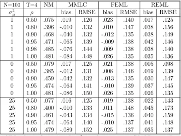
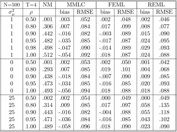
In this section we compare through Monte Carlo simulations the …nite sample properties of four estimators in various panel AR(1) models without covariates: _bC; an asymptot-ically unbiased version of _bF which will be labeled as _bU; the REMLE for that has been proposed by both Chamberlain (1980) and Anderson and Hsiao (1982), henceforth

bREM L; and the FEMLE for (i.e.,bF EM L) that has been proposed by Hsiao et al. (2002).

bU uses the weight matrix WNU de…ned below corollary 2. We study how the properties

of these estimators are a¤ected if we change (1) the distributions of the vi = yi;0 i

or (2) the ratio of the variances of the error components, i.e. 2₌ 2_{. We conducted the}

simulation experiments for (T; N) = (4;100); (9;100); (4;500) or (9;500) and = 0:5;

0:8; 0:9;0:95;0:98or 1:

In all simulation experiments the error components have been drawn from normal distributions with zero means. We assumed that 2 _{= 0;1or25:For the"}

i;t we assumed

homoskedasticity and no autocorrelation: E("i"0i) = 2I with 2 = 1:

In order to assess how the assumptions with respect toyi;0 i,i= 1; :::; N;a¤ect the

properties of the estimators, we conducted two di¤erent sets of experiments, which are identi…ed by a capital: in one set, labeled NS, the initial observations are non-stationary, i.e., yi;0 i = 0,i= 1; :::; N;whereas in the other set, labeled S, the initial observations

are drawn from stationary distributions whenj j<1, i.e.,(yi;0 i) N(0; 2i;0=(1 2))

with 2

i;0 = 2; althoughyi;0 i = 0, i= 1; :::; N; when = 1.

Note that all four estimators su¤er from a weak moment conditions problem when is close to one, cf. Kruiniger (2013).

(1 )vi +"i = (1 ) yi;0 +ui with = 1 for the FE case. In the experiments we

imposed homoskedasticity on their likelihood functions and added the restrictions 2 _>0

and (T 1)(1 )2 2

v + 2 >0to ensure that the estimates of E(uiu0i) were PD.

We allowed for time e¤ects by subtracting cross-sectional averages from the data. We computed _bC and _bU by maximizing elN( ) subject to 1 r 1:4: (We also

tried using 1 r 2 but never found a maximum between 1:4 and 2.) If no local maximum was found, we computed_bC by solving (9) s.t. 1 r 1:4using grid search, and computed _bU by solving (8) withWN =WNU s.t. 1 r 1:4.

Tables 1-6 report the simulation results in terms of the biases and root mean squared errors (RMSEs) of the estimators and the relative frequencies that _bLAN did not exist (NM). The tables di¤er with respect to the dimensions of the panel and the assumptions made about the yi;0 i, i = 1; :::; N. We omitted the results for bU because they are

very similar to those of _bC:Inspection of the results leads to the following conclusions:14

1. In almost all experiments (the exception is design NS with N = 100 and =:0:5)

bREM L is superior in terms of RMSE for ‘smaller’ values of (i.e., values closer to

0), _{bF EM L} is superior for ‘larger’ values of (i.e., values closer to 1), while _bC is superior on an interval of ‘intermediate’ values of , which includes = 0:8 when T = 4 and N = 100; and = 0:9 when T = 4 and N = 500: In most experiments

bREM L is superior when = 0:5; whilebF EM L is superior when is near/equals 1:

When is near 1; the bias of_bC is larger than the biases ofbF EM L and bREM L.

2. When T or N increases, the values of the bounds of the interval for on which_bC

is superior increase. When T = 9 and N = 500; _bC is superior around = 0:95: Furthermore, when = 0:50 and T = 9 or N = 500; _{bF EM L} is often the most e¢cient estimator after_{bREM L}.

3. When 2₌ 2 _{increases, the RMSE of b}

REM L increases and hence the value of the

lowerbound of the interval of values of on which_bC is superior decreases.

14_{Dhaene and Jochmans (2016) report simulations results on the …nite sample properties of}

their Adjusted Likelihood estimator (_bADJ), the bias corrected LSDV estimator of Hahn and Kuersteiner (2002) (_bHK) and the RE GMM estimator of Arellano and Bond (1991) (_bAB). Some of their simulation experiments are equal to some of our experiments. The results for these experiments show that_bADJ and_bC are very similar and that_bHK has a large bias when

4. When V ar(yi;0 i)= 2 decreases, the bias and the RMSE ofbC and the RMSE of

bREM L increase and the value of the upperbound of the interval of values of on

which_bC is superior decreases.

5. The bias of _bU is about the same as the bias of bC; also when is (close to) one.

Moreover, the sign of the bias of _bC is the opposite of the sign that is implied by corollary 1. This suggests that the biases of_bC and_bU are mainly caused by other factors than the random sign of N1=4_{(b 1) when Z}

1 >0:

6. When T = 4 and N = 100; N M > 0:35 for 0:8; when T = 4 and N = 500;

N M > 0:29 for 0:8; when T = 9 and N = 100; N M > 0:35 for 0:9;

and when T = 9 and N = 500; N M > 0:25 for 0:9: Generally, the higher the value of ; the higher the value of N M. When = 1; N M 0:50 for all panels considered, which supports the idea that even asymptotically _bLAN may not exist when = 1. If the value ofV ar(yi;0 i)= 2 decreases, the value ofN M increases.

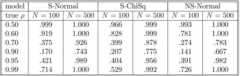
Under design NS, whenT = 4, N = 100 and = 0:5; we still haveN M > 0:3: We have also investigated the size and power properties of the modi…ed likelihood based QLM-test for testingH0 : =a, that is,QLM( ):To this end, we conducted three

types of Monte Carlo experiments. The designs of two of them, labelled S-Normal and NS-Normal, were similar to designs S and NS described above. The designs of the third kind of experiments, labelled S-ChiSq., were also similar to S with one di¤erence: the"i;t were

i.i.d. ( 2_{(1) 1)=}p_{2instead of i.i.d. N(0;1)so that(y}

i;0 i) ( 2(1) 1)=

p

2(1 2₎

instead ofN(0;1=(1 2_{)): In all experiments}

i N(0;1): We used various true values

for including 0:5; 0:9;0:95and 0:99. The results for the power of QLM( )were based on testing H0 : = 0:8. In all experiments T = 9 and N 2 f100;500g.

QLM( )depends on_H(e_n), i.e., an estimate of the expected Hessian that is based on the restricted estimatee_n. One of the parameters in_H( _0;n)is 2

v;n. However, the latter

is not estimated by a MMLE. Instead we used the restricted FE(Q)MLE for 2

v;n.

6

Concluding remarks

Alvarez and Arellano (2004) and Juodis (2013) have extended the MMLE of Lancaster to panel AR(1) models that allow for time-series heteroskedasticity. Their estimators su¤er from the same problems as Lancaster’s MMLE, namely a weak moment conditions prob-lem if the parameter values are close to the unit root and time-series homoskedasticity, cf. Alvarez and Arellano (2004) and Kruiniger (2013); the related problem of possible non-existence; and the possibility of non-uniqueness of local maxima of the modi…ed pro-…le likelihood function. The non-existence problem can be solved by generalizing their estimators in a similar way as Lancaster’s estimator has been generalized to (8) or (9). However, it is unclear whether the modi…ed pro…le likelihood function has at most one lo-cal maximum even when the parameter space for is restricted to[ 1;1].15 _{If uniqueness}

would not hold, then one could select a local maximum that is (plausible and) closest to the value of_bF EM L (orbREM L), which is a consistent estimator, as the MMLE.16

Alvarez and Arellano (2004) and Dhaene and Jochmans (2016) have also extended the MMLE of Lancaster to panel AR(p) models, while Juodis (2013) has also extended the MMLE of Lancaster to panel VARX(1) models. Comments similar to those made in the previous paragraph apply to these extensions. The MMLEs discussed in section 3 are inconsistent for models with endogenous or predetermined covariates. However, in some cases these models can be replaced by VAR models.

It seems reasonable to expect that the aforementioned extensions of the MMLEs to more general models may also outperform the RE- and FEMLEs for those models in panels of realistic dimensions for some parts of the parameter space. However, a compre-hensive Monte Carlo study of their …nite sample properties is left for future research.

Finally, we note that Bester and Hansen (2007) and Arellano and Bonhomme (2009) have proposed priors that result in …rst-order unbiased Bayesian estimators for in a version of model (1) that does not include the K exogenous covariates.

15_{The modi…ed pro…le likelihood equation for is a polynomial in r. If the model has}

no covariates, then the coe¢cients of this polynomial are functions of ; 2

v and T variance

parameters instead of one.

A

Proofs and derivations

The asymptotic bias of the LSDV estimator for ; _{bM L}:

The LSDV estimators for and ; _{bM L} and b_{M L}; satisfy the pro…le likelihood equa-tions for and :

N

X

i=1

y0_{i; 1}Q(yi bM Lyi; 1 XibM L) = 0 and (16) N

X

i=1

X_i0Q(yi bM Lyi; 1 XibM L) = 0:

Let r2

xy 1 = (

PN

i=1y0i 1Qyi; 1) 1PN_i=1(y0i 1QXi)(P_iN₌₁Xi0QXi) 1PN_i=1(Xi0Qyi; 1), s2y =

(T 1) 1_N 1PN

i=1yi;0 1Qyi; 1 and M L =plimN!1bM L:Using that yi; 1 i x0i =

'vi+ QXi + "i =Zei+ "i and Q = 0, it can be shown that the asymptotic bias of

bM L is given by (cf. e.g. Bun and Carree, 2005):

M L =

2_{h( )}

(1 2

xy 1)

2

y

; (17)

where 2

xy 1 = plimN!1r

2

xy 1;

2

y = plimN!1s2y and h( ) = (T 1) 1tr(Q ) =

1

T(T 1)

PT 1

t=1(T t) t 1 =

0

( ):Note thath( ) = _TT_(T1₁₎₍₁T + T₎2;when 6= 1;andh(1) =

1 2:

Assumption 1 implies that 2

y =

2

T 1tr(

0_{Q ) +} 1

T 1E(ZeiQZei)and

2

T 1tr(

0_{Q )>0and}

hence 2

y > 0: We also have 2xy 1 < 1: Furthermore, if 1; h( ) > 0 and hence

M L <0(cf. e.g. Bun and Carree, 2005).

It can also be shown that if = 1; then _{M L} = 3

T+1. Note that E(ZeiQZei) = 2

v'0Q'+2E(vi'0Q QXi) + 0E(Xi0Q Q QXi) :Letf( ) = _T1₁tr( 0Q )and g( ) =

1

T 1'

0_{Q'. Below we show thatf(1) =} 1

6(T + 1): Furthermore,g(1) = 0 and when = 1;

we also have = 2

xy 1 = 0: We conclude that when = 1; then E(ZeiQZei) = 0;

2

y =

2

6 (T + 1) and M L = T+13 (cf. Harris and Tzavalis, 1999).

Proof of the claim that f(1) = 1₆(T + 1) :

We have f( ) = (T 1) 1_tr( 0_{Q ) = (T 1)} 1_(tr 0 _T 1 0 0 _{) = (T 1)} 1

(PT_t=02P_st₌₀ 2s _T 1PT 2

t=0(

Pt

s=0 s)2): It follows thatf(1) = (T 1) 1(

PT 2

t=0 (t+ 1)

T 1PT 1

t=1 t2) = (T 1) 1(12(T 1)T 1

6(T 1)(2T 1)) = 1

Some results related to elc

N(r) and @elc

N(r)

@r :

By the envelope theorem we have @elcN(r)

@r = (r;b

2

(r;b(r));b(r)), i.e.,

@elc N(r)

@r = (T 1)

0

(r) +_b 2(r;b(r))N 1

N

X

i=1

(yi ryi; 1 Xib(r))0Qyi; 1: (18)

Let _b2_{M L} = (T 1) 1_N 1PN

i=1[(yi bM Lyi; 1 XibM L)0Q(yi bM Lyi; 1 XibM L)]:

Next we show that the …rst-order condition for a local maximum ofelc

N(r) can be written

as

@elc N(r)

@r = (T 1)

0_(r) (T 1)(r bM L)

b2M L=(s2y(1 r2xy 1)) + (r bM L)

2 = 0: (19)

Derivation of (19): Using PN_i=1X0

iQ(yi bM Lyi; 1 XibM L) = 0 from (16) and

PN

i=1Xi0Q(yi ryi; 1 Xib) = 0 from (5), we obtain

b_{M L} b= (

N

X

i=1

X_i0QXi) 1 N

X

i=1

(X_i0Qyi; 1)(r bM L): (20)

Next, using PN_i=1y_i;0 ₁Q(yi bM Lyi; 1 XibM L) = 0 from (16), we obtain

N

X

i=1

y_i;0 ₁Q(yi ryi; 1 Xib) = N

X

i=1

y_i;0 ₁Q(yi; 1(bM L r) +Xi(bM L b)) =

(_bM L r)( N

X

i=1

(y0_{i 1}Qyi; 1)

N

X

i=1

(y_i0 ₁QXi)( N

X

i=1

X_i0QXi) 1 N

X

i=1

(X_i0Qyi; 1)):

Hence

(T 1) 1N 1

N

X

i=1

(yi ryi; 1 Xib(r))0Qyi; 1 = (bM L r)s2y(1 rxy2 1): (21)

UsingPN_i=1y0

i; 1Q(yi bM Lyi; 1 XibM L) = 0and

PN

i=1Xi0Q(yi bM Lyi; 1 XibM L) = 0

from (16), we obtain

N

X

i=1

N

X

i=1

[(yi bM Lyi; 1 XibM L)0Q(yi bM Lyi; 1 XibM L)+

((_{bM L} r)yi; 1+Xi(bM L b))0Q(yi; 1(bM L r) +Xi(bM L b))]:

In addition, by using (20) once more, we obtain

N

X

i=1

[((_{bM L} r)yi; 1+Xi(bM L b))0Q(yi; 1(bM L r) +Xi(bM L b))] =

(_bM L r)2[ N

X

i=1

y_i;0 ₁Qyi; 1

N

X

i=1

(y_i0 ₁QXi)( N

X

i=1

X_i0QXi) 1 N

X

i=1

(X_i0Qyi; 1)]:

Hence

b2(r;b(r)) = (T 1) 1N 1

N

X

i=1

(yi ryi; 1 Xib(r))0Q(yi ryi; 1 Xib(r)) =

b2M L+ (bM L r)2s2y(1 r2xy 1): (22)

Finally, combining (18) with (21) and (22) yields (19).

Next we show that 2

M L = plimN!1b2M L >0.

Proof of the claim that 2

M L >0 :

UsingQ(yi bM Lyi; 1 XibM L) =Q("i+ ( bM L)yi; 1+Xi( bM L))andQyi; 1 =

Q(Zei+ "i); where Zei ='vi+ QXi ; we obtain b2M L = (T 1) 1N 1

PN

i=1[("i+ (

bM L)(Zei+ "i) +Xi( bM L))0Q("i+ ( bM L)(Zei+ "i) +Xi( bM L))]:

Assumption 1 implies that "ij(vi; QXi) i:i:d:N(0; 2IT); i= 1; :::; N;with 2 >0:It

follows that 2

M L =plimN!1bM L2 plimN!1(T 1) 1N 1PN_i=1[("i+( bM L) "i)0Q

("i+ ( bM L) "i)] = 2(T 1) 1tr((I+ ( M L) )0Q(I+ ( M L) ))>0:

Proof of the claim that elc

N(r) converges uniformly in probability toelc(r) :

We haveelc

N(r) =elN(r;b2(r;b(r));b(r)) = (T 1) (r) T₂1log(b2(r;b(r))) T₂1 and

from (22), _b2(r;b(r)) = _b2_{M L}+ (_{bM L} r)2_s2

y(1 r2xy 1): Note that log(b

2

(r;b(r))) is a concave function ofr:Then it follows from pointwise convergence oflog(_b2(r;b(r)))to the functionlog( 2_{(r)) log(} 2

M L+( M L r)2 2y(1 2xy 1))that plimN!1supr2[ 1;1) el

c N(r)

Some results related to elc_(r); @elc_(r)

@r j = 0 and @2_e

lc_(r)

@r2 j :

The …rst-order condition for a local maximum of elc_{(r) can be written as:}

@elc(r)

@r = (T 1)

0

(r) ₂ (T 1)(r M L)

M L=( 2y(1 2xy 1)) + (r M L)

2 = 0: (23)

The second-order condition for a local maximum ofelc_{(r)is given by:}

@2e_lc_(r)

@r2 = (T 1)

00

(r) (T 1)(

2

M L=( 2y(1 2xy 1)) (r M L)

2₎

( 2

M L=( 2y(1 2xy 1)) + (r M L)

2₎2 <0:

Below we show that

2

M L=( 2y(1 2xy 1)) =

2 0

( )

2

y(1 2xy 1)

!2

+ 2=( 2_y(1 2_xy 1)): (24)

Then it is easily veri…ed that @el_@rc(r)_j = 0 and

@2e_lc_(r)

@r2 j = (T 1)

00

( ) + (T 1)(2 ( 0( ))2 2_y(1 2_xy 1)=

2_):

Note that(T 1) 2

y = 2tr( 0Q ) +E(ZeiQZei). Let x2 =plimN!1 _(T 1_1)N PN_i=1Xi0QXi

and 2

xy 1 =plimN!1

1 (T 1)N

PN

i=1Xi0Qyi; 1:UsingQyi; 1 =Q(Zei+ "i)it is easily seen

that 2

y(1 2xy 1)=

2 _{= (} 2

y 0xy 1

2

x xy 1)=

2 _{(T 1)} 1_tr( 0_{Q ); with equality}

holding if = 1 or 2

v = = 0 (i.e. if zqz = 0): We also have 00( ) (T 1) 1

tr( ( )0_{Q ( )) + 2(} 0_{( ))}2 _{0; with equality holding if = 1 or T = 2: It follows that}

@2_e

lc_(r)

@r2 j 0; with equality holding if = 1or if T = 2 and

2

v = = 0: Thuselc(r) has a

local maximum at when ₆= 1 and, in case T = 2, zqz >0. Below we show thatelc(r)

has a stationary point of in‡ection at when = 1.

Derivation of (24): Given that the equality yi ryi; 1 Xib = ( r)yi; 1+Xi(

b) + i +"i holds for any r and b; including for r =bM L and b = bM L, we can rewrite

b2M L as

b2M L= (T 1) 1N 1 N

X

i=1

[(( _bM L)yi; 1 +Xi( bM L) +"i)0

Let _{M L} = plimN!1bM L; 2x = plimN!1(T 1) 1N 1PN_i=1Xi0QXi; and 2xy 1 =

plimN!1(T 1) 1N 1PN_i=1Xi0Qyi; 1: Then combining plimN!1N 1P_iN₌₁Xi0Q(yi

bM Lyi; 1 XibM L) = 0 from (16) with plimN!1N 1PN_i=1X_i0Q(yi yi; 1 Xi ) =

plimN!1N 1PiN=1Xi0Q"i = 0 gives

M L = x2 xy 1( M L): (26)

Using (25) and (26) and recalling that 0( ) =h( ) = (T 1) 1_{tr(Q ), we obtain}

2

M L= p lim N!1b

2

M L = ( M L)2 2y+ 2( M L)0 xy 1( M L)+

( _{M L})0 2_x( _{M L}) + 2( _{M L}) 2(T 1) 1tr(Q ) + 2 = ( _{M L})2 2_y 0_xy 1

2

x xy 1( M L)

2_{+ 2(}

M L) 2(T 1) 1tr(Q ) + 2 =

( _{M L})2 2

y(1 2xy 1) 2( M L)

2 0_{( ) +} 2_:

Finally, using _{M L} = 2 2 0( )

y(1 2xy 1)

; we …nd that

2

M L=( 2y(1 2xy 1)) =

2 0_{( )}

2

y(1 2xy 1)

!2

+ 2₌₍ 2

y(1 2xy 1)):

Proof of the claim that elc_{(r) has an in‡ection point at when = 1 :}

We have already seen that @el_@rc(r)_j =1 = @

2_e

lc_(r)

@r2 j =1 = 0:In addition, we have

@3_elc_(r)

@r3 = (T 1)

000_{(r) +} 6(T 1)(r M L)( 2M L=( 2y(1 2xy 1))) ( 2

M L=( 2y(1 2xy 1)) + (r M L)

2₎3

2(T 1)(r _{M L})3

( 2

M L=( 2y(1 2xy 1)) + (r M L)

2₎3;

000

(1) = (T 2)(₁₂T 3); f(1) = T+1₆ ; 0(1) = ₂1; lim !1 2xy 1 = 0; lim !1( M L ) = 0₍₁₎

f(1) = 3

T+1 and lim !1( 2M L=( 2y(1 2xy 1))) =

0₍₁₎

f(1) 2

+ _f(1)1 = 3(2_(TT₊₁₎1)2: It follows that

@3_e

lc_(r)

@r3 j =1 = (T 1)

000_{(1) +} (T 1)2

2 6= 0 (in fact >0) for T 2:

We now present two lemmata that help to establish uniqueness and consistency of our MMLEs:

maximum, namelybW =bC, and one local minimum on the set e w.p.1. (ii)elcN(r) has

either no local optima or one local maximum, namely _bW =_bC, and one local minimum on the interval [ 1;₁) w.p.1. (iii) The equation @elcN(r)

@r = 0 has either no solution on

[ 1;₁) or two solutions on [ 1;₁), namely _b1 and_b2 with_b1 <_b2 and_b1 =_bW =_bC, w.p.1.

Lemma 2 Let Assumption 1 hold. First let ₆= 1: Then (i)el( ) has one local maximum and one local minimum but no in‡ection point on the set e. The local maximum is

attained at 0. (ii)elc(r)has one local maximum and one local minimum but no in‡ection point on the interval [ 1;1). The local maximum of elc_{(r) is attained at . (iii) The}

equation @el_@rc(r) = 0 has two solutions on [ 1;₁): ₁ and ₂ with ₁ < ₂ and ₁ = :

Now let = 1:Then (iv)el( ) has one stationary point of in‡ection but no local optima on e. The in‡ection point is attained at 0. (v)elc(r)has one stationary point of in‡ection but no local optima on [ 1;1). The in‡ection point of elc_{(r) is attained at = 1. (vi)}

The equation @el_@rc(r) = 0 has only one solution on [ 1;₁): ₁ = 1:

We …rst prove the following lemma, which summarizes some useful properties of 0( ) :

Lemma 3 Let 1: When T 2; 0( )>0; 0(1) = 1 2; When T = 2; 0( ) = 1₂;

When T = 3; 0( 1) = 1 6 and

00_{( ) =} 1 6;

When T 4 and T is even, 0( 1) = _2(T1 ₁₎; 00( 1) = 0; 00( ) > 0 when > 1;

and 000( )>0;

WhenT 5 andT is odd, 0( 1) = ₂1_T; 00( )>0; 000( 1) = T_4T3 <0; 000( 1=2) =

24 T₍₂T _3T+1)

27T(T 1) > 0; and 9 with 1 < < 1=2 such that

000_{( ) = 0;} 000_{( ) < 0 for}

< and 000( )>0 for > :

Proof of lemma 3: for the proof of most properties see Dhaene and Jochmans (2015). Their proof uses that 0( ) = [T(T 1)] 1PT 1

t=1 (T t) t 1 =

T 1 T + T

T(T 1)(1 )2 when

6

= 1; and Descartes’ rule of signs. The remaining claims, i.e., 0( ) = 1

2 when = 1 or

T = 2; 00( ) = 1

6 when T = 3;

0_{( 1) =} 1

2(T 1) whenT is even, and

0_{( 1) =} 1

2T when T

is odd, are easily veri…ed.

Thus when 1; we have:

If T = 3;then 0( ) is strictly positive and increasing linearly;

IfT 4and T is even, then 0( )is strictly positive, non-decreasing and strictly convex; If T 5 and T is odd, then 0( ) is strictly positive, strictly increasing and …rst strictly concave and then strictly convex.

Proof of lemma 1:

We can write (19) as

0

(r)fb2M L=(sy2(1 rxy2 1)) + (r bM L)

2_{g= (r}

bM L): (27)

Let _N(r) = 0(r)fb2M L=(s2y(1 rxy2 1)) + (r bM L)

2_{g: Then} 0 N(r) =

00

(r)fb2M L=(s2y(1

r2

xy 1)) + (r bM L)

2_{g+ 2(r b}

M L) 0

(r) and 00_N(r) = 000(r)_fb2_{M L}=(s2

y(1 r2xy 1)) + (r

bM L)2g+ 4(r bM L) 00

(r) + 2 0(r):

By lemma 3 _N(r) > 0 when r 1. Hence any solution r of (27) should satisfy r >_{bM L}. When r max( 1;_{bM L}); we also have by lemma 3 that 0_N(r)>0and if T is even that 00_N(r)>0while if T is odd we either have _N00(r)>0for all r max( 1;_{bM L})

or 00_N(r) < 0 for all r on [max( 1;_{bM L}); ) and 00_N(r) > 0 for all r on ( ;₁) with > max( 1; M L) and equal to the solution of 00N(r) = 0. It follows that w.p.1. the

graph of N(r)either does not intersect the liner bM L (this may well happen when is

close or equal to unity, see Lancaster for an example) or intersects the liner _bM L twice,

say at r = _b1 and r = _b2 with max( 1;_{bM L}) < _b1 < _b2: Both solutions of (27) would correspond to local optima w.p.1. That is, the possibility that r _{bM L} is a tangent to

N(r)atb1 and/orb2 is an event with probability zero, sob1 andb2 would not correspond

to (an) in‡ection point(s) w.p.1. It is clear that when 1;elc

N(r) andelN( ) attain at

most one local maximum on the interval[ 1;₁) and the set e, respectively. Moreover, if (27) has any solutions, then _bC is one of them and _bC =_bW max( 1;_{bM L}). Given that elc

N(r) has a global maximum at r = 1 (because limr"1elcN(r) = 1), we conclude

that if (27) has any solutions, then it has two solutions _b1 and _b2 with _b1 < _b2, where

b1 = bC = bW corresponds to a local maximum of elcN(r) and b2 corresponds to a local

minimum ofelc

N(r); becauseelNc (r) cannot attain a local maximum atb2. Likewise, given

that limr"1elN(b(r)) = limr"1elcN(r) = 1; we conclude that if (27) has solutions b1 and

b2 with b1 < b2, then elN( ) has two local optima on the set e; say b1 and b2; where

b₁ =b(_b1) = b(_bW) = b(_bC) corresponds to a local maximum of elN( ) and b2 = b(b2)

corresponds to a local minimum of elN( ), becauseelN( ) cannot attain a local maximum