An evolutionary algorithm for graph planarisation by vertex deletion

Rodrigo Lankaites Pinheiro

, Ademir Aparecido Constantino

, Candido F. X. de Mendonc¸a

and Dario Landa-Silva

1_{School of Computer Science, University of Nottingham, NG8 1BB, Nottingham, U.K.}

2_{Informatics Department, State University of Maring´a, Maring´a, PR, Brazil}

3_{School of Arts, Science and Humanities, USP-East, S˜ao Paulo, SP, Brazil}

[email protected], [email protected], [email protected], [email protected]

Keywords: Graph Planarisation, Evolutionary Algorithms, Vertex Deletion.

Abstract: A non-planar graph can only be planarised if it is structurally modified. This work presents a new heuristic algorithm that uses vertices deletion to modify a non-planar graph in order to obtain a planar subgraph. The proposed algorithm aims to delete a minimum number of vertices to achieve its goal. The vertex deletion number of a graph G= (V,E)is the smallest integer k≥0 such that there is an induced planar subgraph of G obtained by the removal of k vertices of G. Considering that the corresponding decision problem is NP-complete and an approximation algorithm for graph planarisation by vertices deletion does not exist, this work proposes an evolutionary algorithm that uses a constructive heuristic algorithm to planarise a graph. This constructive heuristic has time complexity of O(n+m), where m=|V|and n=|E|, and it is based on the PQ-trees data structure and on the vertex deletion operation. The algorithm performance is verified by means of case studies.

1

INTRODUCTION

Practical applications of Graph Drawing, such as the design of VLSI circuits, requires drawing techniques for non-planar graphs. A graph (representing the cir-cuit) needs to be drawn on the plane (an electronic chip) without crossing edges. However, graph draw-ing algorithms are restrained to planar graphs, oth-erwise the results obtained by these algorithms are compromised. Network design and analysis and com-putational geometry are additional well known fields where the drawing of planar graphs are required. A possible way to tackle non-planarity in graphs is to consider its topological invariants, such as the number of vertex deletion, which can be used as the measure of non-planarity.

The simple drawing of a graph G= (V,E) is a drawing of G on the plane, where each edge does not cross itself, adjacent edges do not cross themselves, the crossing of two edges only occurs once, the edges do not cross over vertices, and no more than two edges cross at the same point. A graph is considered planar when there is a simple drawing for this graph on the plane, without crossing edges. Without loss of gen-erality, from now on we are considering only simple drawings.

Take all drawings of G, the drawing which pos-sesses the lowest number of edge crossings among all drawings is named optimal drawing of G. And the number of edge crossings is named crossing number of G, denoted by cr(G).

The number of vertex deletionΦ(G)is the small-est integer k>0 such that the deletion of k vertices from G produces a planar graph. The decision prob-lem regarding the number of vertex deletion, the num-ber of vertex splitting, the numnum-ber of edges deletion and the crossing number are all NP-complete (Faria et al., 2001a; Garey and Johnson, 1983; Liu and Geld-macher, 1977; Yannakakis, 1978). (Faria et al., 2006) proved that an approximation algorithm cannot exist for the graph planarisation problem using the vertex deletion operation, hence a heuristic algorithm be-comes a viable alternative to tackle the problem. Also it has been shown that it remains NP-hard even for cubic graphs (Faria et al., 2001a; Faria et al., 2001b; Faria et al., 2004). Besides, (de Figueiredo et al., 1999) showed that the same occurs for the number of vertices splittings according to the result obtained by (Robertson and Seymour, 1995).

Marek-Sadowska, 1978; Ozawa and Takahashi, 1981; Pasedach, 1976). One of the best approaches is the

PLANARISE algorithm by (Jayakumar et al., 1989)

referred as JTS PLANARISE algorithm. The JTS

PLA-NARISE algorithm is based on the planarity test

al-gorithm by (Lempel et al., 1967) and (Even, 2011) (also referred as the LEC algorithm) and its imple-mentation using PQ-trees (Booth and Lueker, 1976). (Eades and de Mendonc¸a, 1993) considered the num-ber of vertex splittings adapting the PLANARISE al-gorithm into the SPLIT-PLANARISE. That was done by replacing the edge removal operation for the vertex splitting operation. Both algorithms have time com-plexity O(n2)and space complexity O(n+m), where

n represents the number of vertices and m represents

the number of edges of G. This work proposes an al-gorithm named VD-PLANARISE which uses similar ideas to the JTS PLANARISE algorithm above men-tioned, though it uses the operation of vertex deletion instead of edge removal. In the next section it will be discussed how the JTS PLANARISE algorithm was adapted for the new proposed constructive heuristic which has time and space complexity of O(n+m). We can also highlight that the JTS PLANARISE algo-rithm generates a planar subgraph where the proposed algorithm generates an induced planar subgraph.

Section 2 describes a few necessary concepts. In section 3 we present the VD-PLANARISE algorithm. The section 4 analyses the complexity and the perfor-mance of the proposed algorithm. Section 5 presents the evolutionary algorithm MAVD-PLANARISE and later we show an empirical analysis of the performed tests of the proposed algorithms (section 6).

2

THE LEC ALGORITHM AND

PQ-TREES

This section presents the basics of the JTS

PLA-NARISE algorithm, which is based on the LEC

pla-narity test algorithm which is performed with the aid of PQ-trees. The definitions of the data structure and its operations are described in this section. However, for further details on the implementation of the opera-tions on PQ-trees we recommend the work of (Booth and Lueker, 1976).

The LEC algorithm only deals with biconnected graphs. Considering that it is fairly easy to divide a graph into a tree of biconnected components (blocks), (Gibbons, 1985) presents a linear complexity algo-rithm for the generation of a tree of biconnected com-ponents for a given graph. This work may consider, thus, only biconnected graphs.

Take a biconnected graph G= (V,E)with n=|V|

vertices and m=|E| edges. An st-numbering is a labeling of the vertices in G with integer numbers 1,2, ,n where 1 is adjacent to n and a vertex

num-bered j is adjacent to a pair of vertices numnum-bered i and k where i< j<k. The vertex 1 is named source

and is referred as s while the vertex n is named sink and is referred as t. Each biconnected graph has a

st-numbering (Lempel et al., 1967) and such labeling

can be found in linear time (Even and Tarjan, 1976). The graph G labeled with numbers is named st-graph.

Let Gk, where 1≤k≤n, be a subgraph of an

st-graph G induced by the set of vertices Vk=1,2, ...,k.

Let Bkbe a graph associated with the subgraph Gkand

all of the edges of G connected with the vertices Vk

and V−Vkin G. These edges are named virtual edges

and the vertices V−Vkare named virtual vertices. The

virtual vertices are labeled as its original vertices in G; though they remain apart (a leaf for each adjacent ver-tex not yet embedded). Consequently, in Bkthere may

be several virtual vertices with the same label, each of them with exactly one virtual edge. A drawing Bkis

named bush form of Gkif the vertices with smaller or

equal labels than k appears at a higher level than the leaves and all of the virtual vertices appears as leaves. It is possible to demonstrate (Even, 2011; Lempel et al., 1967) that a st-graph is planar if and only if for each Bk, 2≤k≤n−2, there is a planar graph B′k

isomorph to Bksuch that all the virtual vertices in B′k

labeled k+1 appear consecutively.

A PQ-tree (Booth and Lueker, 1976) T is a data structure that represents a set of permutations in a set

S. The nodes of T can be leaves, representing the

elements of S; P-nodes, conventionally represented as a circle; and Q-nodes, conventionally represented as a rectangle.

For this kind of tree the order that the descendants of a node appear is important. The borderline of T is defined as the permutation represented by the order of the leaves of T from left to right. For example, the borderline of the first PQ-tree in Figure 1 is[abcde].

The set of permutations represented by T is gen-erated by rearranging the descendants of each node P and Q, according to two rules – the descendants of a

P-node can be freely permuted and the order of the

descendants of a Q-node can only be inverted. The set of permutations of S represented by T is the set of borderlines of the PQ-trees obtained from

T , by rearranging the descendants according to these

rules. For example, the set of permutations repre-sented by the PQ-tree in Figure 1 is:[abcde],[abced],

[cbade],[cbaed],[dabce],[dcbae],[eabcd],[ecbad],

[deabc],[decba],[edabc], and[edcba].

prob-Figure 1: The twelve permutations allowed for the given PQ-tree.

lems involving a successive reduction of the set of permutations to find a specific permutation. For ex-ample, they have been used to identify planar graphs, interval graphs, matrix with the property of consecu-tive ones (Booth and Lueker, 1976), hierarchical pla-nar graphs (Battista and Nardelli, 1988), as well as the dominance drawings (Eades and de Mendonc¸a, 1993).

In this work, a PQ-tree Tkis used to represent the

bush form Bkin the algorithm. The nodes of Tk

corre-spond to the following:

• leaves: the virtual vertices of Bk;

• Q-nodes: the maximal biconnected components

in Bk; and

• P-nodes: the articulation vertices in Bk.

The leaves are named pertinent if they correspond to the next selected vertices (label k+1) with the pos-sibility to be embedded, while the others are named non-pertinent leaves. In the same way, a non-leaf node X is pertinent if any leaf descendant of X in the

PQ-tree is pertinent. If all the leaves from the

descen-dants of a node X in the PQ-tree are pertinent, then

X is named a full node. If no leaf descendant of the

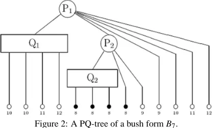
node X is pertinent then X is empty. The X border-line is defined by its set of descendant leaves, read from left to right. A node X is a pertinent root if it is the lowest level node whose borderline has only per-tinent leaves. The tree rooted in X is named perper-tinent subtree. Once a pertinent root is identified, a series of pattern tests and reallocations described in (Booth and Lueker, 1976) can be used in order to build a new tree in which all the pertinent leaves are shown consecu-tively if such tree exists. In this case all the pertinent leaves in the new tree will appear as descendants of a single node. For instance, suppose that the PQ-tree from Figure 2 represents a bush form B7; P1 node is

a pertinent node; Q1 node is an empty node; P2 node

is the pertinent root; Q2 node is a full node; the per-tinent leaves are labeled as 8; and the non-perper-tinent leaves are labelled as 9,10,11,12.

Figure 2: A PQ-tree of a bush form B7.

Reduction is an important operation of a PQ-tree. On an abstract level, the reduction takes a set of per-mutationsΠ of S and a subset S′⊆S and returns a

subsetΠ′ofΠin a way that the elements of S′ con-secutively appear in all the permutations inΠ′. The elements of S′are named pertinent elements of S.

(Booth and Lueker, 1976) created an algorithm that reduces a Tktree into a Tk∗tree in a way that all the

pertinent leaves consecutively appear in the border-line (when possible). The reduction operation can be efficiently executed with a sophisticated implementa-tion of PQ-trees. This work, however, does not dis-cuss these operations that are detailed in (Booth and Lueker, 1976).

It is trivial to notice that not always a PQ-tree Tk

can be reduced into a T_k∗, thus (Ozawa and Takahashi, 1981) defined some criteria to test a tree before ap-plying the reduction. Let G be a biconnected st-graph and T1,T2,,Tn−1be the PQ-trees corresponding to the

bush forms B1,B2,,Bn−1of G. A node X of a PQ-tree

is classified according to its borderline, as follow:

• Type A: if the rooted subtree in X could be

de-scendant of X consecutively appear in the middle of the borderline, with at least a non-pertinent tree in each extreme of the borderline. For example, the P1node in Figure 2 is the type A.

• Type B: if the borderline of the rooted subtree in X consists only of pertinent nodes, then X is a full

node. For example, Q2node in Figure 2 is type B. • Type H: if the rooted subtree in X could be

rear-ranged in a way that all the pertinent leaves de-scendant of X consecutively appear in one of the ends of the borderline. For example, P2node in

Figure 2 is type H.

• Type W: if the borderline of the rooted subtrees in X consists only of non-pertinent leaves, that is, X

is an empty node. For example, Q1node in Figure

2 is type W .

It is known that a PQ-tree is not always one of the types A, B, H or W . However, the need to transform (essentially by vertex deletion) the whole tree in a tree of the W type will be further looked at.

A graph G containing n vertices is planar if and only if the pertinent roots in all the PQ-trees,

T2,T3,,Tn−2 of G are of the B, H or A type. A

PQ-tree is reducible if its pertinent root is of B, H or A type, otherwise, it is irreducible (Ozawa and Taka-hashi, 1981).

Both T1and T2 trees are reducible. The first one

because it has just a pertinent leaf corresponding to the edge(v1,v2), and the second one because it has

only one type of leaf that is the node corresponding to the virtual vertex n.

3

PLANARISATION BY VERTEX

DELETION

In this section we introduce the proposed graph planarisation constructive heuristic VD-PLANARISE which uses the vertex deletion operation.

In general, the VD-PLANARISE algorithm starts with a vertex and continues with the insertion of one vertex at a time, building an induced planar subgraph

G′of G. The vertices are selected following the label-ing order introduced by the st-numberlabel-ing algorithm (Lempel et al., 1967). Let v be the next candidate ver-tex to be inserted in the planar subgraph G′. Let Ev

be the edge subset incident with the vertex v and the vertices of G′and let ˆEvbe the subset of other edges

incident with v. For each iteration if a vertex v cannot be inserted into G′then it is removed. The remaining set of edges(v,u)∈_Eˆ_{vis added (as dummy edges) to} the first inserted vertex (vertex 1). This will be done

to each u vertex that does not have another adjacent with a smaller label comparing to the v label, aiming to maintain the property of st-numbering.

The proposed algorithm is presented as follows:

VD-PLANARISE Input: graph G.

Output: an induced planar subgraph of G. Pre-processing: obtain a valid st-numbering of G, obtain small(u) for every vertex u in G.

Begin:

build the initial tree T1; for k:=2 to n-2 do: {following the st-numbering}

if Tk−1 is reducible then: reduce;

else

Update(vk);

obtain Tk by replacing every pertinent node from T_k−1∗ by a new P-node Pk such as every edge adjacent to the vertex

vk with label higher than k

appears as a direct descendant of Pk.

return G; End.

The algorithm starts with the T1tree and builds the

sequence of PQ-trees T2,T3,. If a graph is planar the

LEC algorithm finishes after building the Tn−1tree,

otherwise it finishes when it detects the impossibility to reduce a Tktree into T_k∗.

Consider Tkan irreducible PQ-tree of a non-planar

graph, that is, it is impossible to reduce a Tktree into T_k∗. The proposed algorithm adds a new operation named Update(k). This operation removes all the per-tinent leaves transforming the Tktree in type W .

Be-sides, if any u vertex with a label higher than k+1, adjacent to the equivalent vertex of the removed per-tinent leaves does not have any other adjacent vertex with a smaller label, a new edge (dummy) is added to the graph in a way that u is adjacent to s. This is nec-essary to maintain the property of st-numbering. Each immersion iteration of the algorithm can increase the number of the adjacent vertices of s. However, this number does not exceed the number of vertices in G. The main question is how to inspect the adjacency of the vertices to be removed in order to assure the prop-erty of st-numbering without increasing the complex-ity of time. This can be done by adding a small(u)

field to each vertex u. This field informs the amount of u adjacents with smaller labels than the u label es-tablished in the step of st-numbering. Thus, when the pertinent nodes -correspondent to the vk+1vertex - are

When the value of the small(u)field reaches zero, a dummy edge is added from s to u. After the last itera-tion, all the dummy edges from s to u are removed for vertex where small(u)field is zero.

4

TIME COMPLEXITY AND

PERFORMANCE OF THE

VD-PLANARISE

The Booth and Lueker reduction of all reducible PQ-trees Tkcan be performed in a total time of O(n+m)

(Jayakumar et al., 1989). If a PQ-tree Tk is not

re-ducible, the Update(k) operation that will remove the pertinent vertices is performed. Suppose the worst case with the maximum of removed vertices (notice that it is true for the Kngraph). In this case, for each v vertex removed the algorithm inspects the labels of

each adjacent vertex u of v. If the label of u is larger than the label of v, a unit is reduced to the small(u)

value. Thus the Update(k) operation will inspect each vertex and its adjacents (like BFS algorithm). Hence in the worst case the total time of this operation is

O(n+m). The addition of dummy edges to the s ver-tex is done in the worst case n times. Therefore the complexity of time of VD-PLANARISE is O(n+m).

Since the proposed algorithm is a heuristic one, questions may arise regarding the quality of its solu-tions, i.e. the amount of vertices removed. The algo-rithm efficiency - with the exception of a few cases such as the complete graph Kn- is highly dependable

on the st-numbering, since the PQ-trees are built in that order. Hence remains the question: how many different st-numberings can a graph possess? And what is the impact of different st-numberings regard-ing the quality of the obtained solutions?

It is not trivial to answer these questions since the number of st-numberings of a given graph varies ac-cordingly to its structure and characteristics. For a complete graph consisting of n vertices, after the st edge is chosen each vertex without a label can be a candidate to receive the next label, thus it is trivial to show that there are n! possible st-numberings for such graph. It is easy to see that for that case different st-numberings does not affect the solution since every vertex is adjacent to every other vertex, however we can use n! as an upper bound to the number of possi-ble st-numberings.

Therefore, given the large st-numbering possibil-ities space and knowing that different st-numbering affects the quality of the solutions obtained by the

VD-PLANARISE, we decided to use a search

tech-nique to refine the solutions. For additional details

regarding the VD-PLANARISE algorithm we recom-mend the work of (Constantino et al., 2011) and (Pin-heiro et al., 2012).

5

THE EVOLUTIONARY

ALGORITHM

MAVD-PLANARISE

As the VD-PLANARISE algorithm possesses linear time complexity, its use as an objective function for optimisation techniques is efficient enough. Know-ing that it is possible to run a st-numberKnow-ing algo-rithm with linear time complexity and that the st-numberings possibilities space is too large to enumer-ate, the use of an enhanced mechanism to search a large solution space is viable. Hence we propose the

MAVD-PLANARISE.

The objective of the MAVD-PLANARISE is to search for the best parameter setup for both the st-numbering and VD-PLANARISE algorithms. The

MAVD-PLANARISE is defined over the basic

struc-ture of a memetic algorithm, consisting of a genetic algorithm (Goldberg, 1989) and a local search. The individuals are defined in a structure that contains a copy of the adjacency structure of the graph to be pla-narised, a(s,t)edge to be used in the st-numbering algorithm, a st vector containing the st-numbering of the graph over that setup and the fitness value (number of removed vertices) calculated after the st-numbering.

The chromosome of an individual is a copy of the adjacency list of the given graph. Let G be a graph and c be a chromosome; c consists of n genes where

n is the number of vertices of G. Each gene gkis the

adjacency list of the vertex vk.

Every time an individual is generated - over the initial population generation or by crossover - the

st-numbering algorithm is applied over its adjacency

structure using the individual selected(s,t)edge with the purpose of obtaining the st-numbering, which is stored in the st vector. After the st-numbering is ob-tained, the fitness value is then calculated using the

VD-PLANARISE algorithm. Only after that procedure

chances of less fit individuals and avoid stagnation, the algorithm also utilises a linear scaling (Goldberg, 1989) technique to calculate the fitness value.

Regarding the selection process, after defining the elite, the algorithm uses the roulette method (Gold-berg, 1989) to select the pairs for crossover. The se-lection process using the roulette method uses the fit-ness value tk= fscaling(fO(k))of each individual of

the actual population and the total value ts=∑nk=1tk,

where n is the number of individuals of the popula-tion. After calculating those values a random value r is picked where 1≤r≤ts and the algorithm selects

the individuals that belong to the range of the sum of the picked number.

The crossover mechanism of the proposed algo-rithm is composed by two steps. The first one is a regular uniform crossover operation (Goldberg, 1989) and the second one is what defines the method as a memetic algorithm, a local search to find the best

(s,t)edge to be used by the st-numbering algorithm. After the chromosomes are generated and before cal-culating the fitness, every new individual has a small chance of suffering a mutation. Let this chance beα. The mutation process uses the flip technique where one gene is randomly raffled and all the adjacency list of that chosen gene is shuffled.

After the crossover, the MAVD-PLANARISE run a greedy local search procedure for each individual on the neighbourhood of the(s,t)edge with the purpose of choosing the best edge for that graph structure. The procedure begins its search by picking up the best

(s,t)edges from the individual parents. The choosing of this edge is made during the crossover and the pro-cess consists of finding the best st-numbering given the edge (s,t) and the inverse (t,s) of each parent and the adjacency structure of the generated individ-ual. Only then the greedy search starts by the selected

(s,t)edge, its st-numbering and the resulting num-ber of vertices of the graph planarisation using that setup. For each vertex v adjacent to s the

GREEDYST-SEARCH algorithm generates a st-numbering using

the edge(s,v)as a temporary(s,t)edge and planarise the graph using the VD-PLANARISE algorithm. If the resulting planar subgraph has more vertices than the one with the original(s,t)edge, then the vertex

v replaces the vertex t in the(s,t)edge. The greedy search also executes the same procedure for the edge

(v,s) and in case the obtained planar subgraph has

more vertices than the original one,(s,t):= (v,s)and the GREEDYST-SEARCH algorithm return its recur-sive call over the new(s,t)edge. The algorithm ends when it cannot find a better solution.

Figure 3: Results for Cn×Cmgraphs.

6

RESULTS

We tested the algorithms on two types of graphs; cartesian graphs, for they possess symmetric and cyclic characteristics among its vertices and edges and randomly generated graphs. For each n, where 3≤n≤10, we generated ten Cn×Cm graphs with m evenly spread through[n,25], hence obtaining 80 graphs. As for the random graphs, we generated 200 graphs, with |V| evenly distributed such that 30≤ |V| ≤75 and for each pair of vertices we set an edge with a probability ofδ, where each graph was given a randomδvalue such that 0.25≤δ≤0.75.

As for a measure, we tested the VD-PLANARISE for every possible st-numbering using an enumeration algorithm. The comparative of the quality of the solu-tions was made between the average and the best lutions obtained by the VD-PLANARISE, and the so-lution obtained by the MAVD-PLANARISE. Regard-ing the parametrisation of our proposed memetic al-gorithm, we defined a population of 100 individuals, and a variable mutation rateαproportional to the pop-ulation’s stagnation, such that 0.05≤α≤0.15. For each graph we run the algorithm three times and used the second better result.

Figure 3 presents the chart with the results ob-tained from the tests on the Cn×Cm graphs. The

first interesting observation is regarding the dis-crepancy between the average solutions obtained by the VD-PLANARISE and the solutions found by the

MAVD-PLANARISE, meaning that the different

Table 1: Summary of the experiments.

numberings in fact have great impact over the quity of the solutions obtained by the planarisation al-gorithm. Furthermore, we can conclude that for this special class of graphs, the algorithm performs well enough to, in every test case, improve the quality of the obtained solutions.

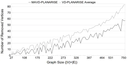
Figure 4 shows the results obtained from the tests on random graphs. Again, we can observe that the proposed metaheuristic was able to search the solu-tion space and find better solusolu-tions.

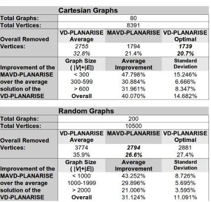
Table 1 presents a summary of the experiments. For cartesian graphs, we can highlight that the so-lutions obtained by the MAVD-PLANARISE are very close to the optimal solutions of the VD-PLANARISE, overall only 0.7% worse, hence proving the quality of the proposed algorithm for this type of graphs. For the random graphs, it can be seen that the perfor-mance of the MAVD-PLANARISE is superior to the optimal solution found testing all the st-numberings. This happens because the algorithm not only search in the space of possible st-numberings, but also changes the visiting order of the vertices, which affects di-rectly the PQ-trees algorithms and therefore the

VD-PLANARISE.

The table also presents the mean of the

improve-Figure 5: Time curve for the MAVD-PLANARISE.

ments achieved by applying the metaheuristic and comparing it to the average solution obtained by the

VD-PLANARISE. We can observe that as the size of

the graph increases, so the improvement of the solu-tions obtained by the metaheuristic decreases. This is expected as the search space increases and the prob-lem gets more difficult. Nonetheless, the algorithm performs similar both on cartesian and random graphs as the overall improvements for cartesian graphs was 40.07% with a standard deviation of 14.682% and for random graphs with similar size range as the carte-sian graphs was 43.252% with a standard deviation of 8.726%.

The algorithm execution time is shown by the Fig-ure 5 using different sized graphs in terms of number of vertices and edges (|V|+|E|) and the execution time in seconds. It can be noted that the algorithm has a polynomial time performance, with a slightly non-linear growing curve.

7

CONCLUSION

This work presented an evolutionary algorithm for graph planarisation - MAVD-PLANARISE - which is based on memetic algorithms. As the planarisation heuristic algorithm, the proposed algorithm applies the VD-PLANARISE which uses the vertex deletion operation to obtain a planar subgraph. To the best of our knowledge this is the only algorithm found in the literature which optimises the number of vertices to be removed for the process of graph planarisation.

It is important to emphasise that in the literature, no linear complexity algorithm that planarises a graph by removing vertices can be found as the use of the vertex deletion operation is not frequent. Note that the proposed algorithm finds an induced planar subgraph from bi-connected non-planar components. However it is possible to find a tree (or a forest in case the graph is not connected) of bi-connected compo-nents in linear time complexity and build an induced planar subgraph using successive applications of the algorithm VD-PLANARISE. Hence the algorithm proposed here represents a sound and novel approach to graph planarisation using the vertex deletion.

also runs a local search on each individual, further improving the results.

Future research include improvements on the memetic algorithm in order to investigate a wider search space, not just the one provided by the

VD-PLANARIZE. One option is to use the final solution

of the MAVD-PLANARIZE as a starting point to another search procedure (such as simulated

anneal-ing, GRASP, VNS, PSO, etc) that does not rely on

the VD-PLANARIZE, but instead search in different neighbourhoods. Another option is to adapt such neighbourhoods to the local search procedure already presented in this work. In any case, investigating a wider range of neighbourhoods could potentially improve the quality of the obtained solutions.

REFERENCES

Battista, G. D. and Nardelli, E. (1988). Hierarchies and planarity theory. IEEE Transactions on Systems, Man, and Cybernetics, (18):10351046.

Booth, K. S. and Lueker, G. S. (1976). Testing for the con-secutive ones property, interval graphs, and graph pla-narity using pq-tree algorithms. Journal of Computer and System Sciences, 13(3):335 – 379.

Chiba, T., Nishioka, I., and Shirakawa, I. (1979). An al-gorithm of maximal planarization of graphs. In Proc. 1979 IEEE Symp. on Circuits and Sys, pages 649–652. Constantino, A. A., de Mendonc¸a, C. F. X., and Pinheiro, R. L. (2011). Um algoritmo heurstico de complex-idade linear para planarizac¸o de grafos por remoc¸o de vrtices. In In Proc. XLIII Simp´osio Brasileiro de Pesquisa Operacional, XLIII SBPO, pages 1–11. de Figueiredo, C. M. H., Faria, L., and Mendonc¸a, C. F. X.

(1999). Optimal node-degree bounds for the complex-ity of nonplanarcomplex-ity parameters. In Proceedings of the tenth annual ACM-SIAM symposium on Discrete al-gorithms, SODA ’99, pages 887–888.

Eades, P. and de Mendonc¸a, C. F. X. (1993). Heuristics for planarization by vertex splitting. In In Proc. ALCOM Int. Workshop on Graph Drawing, GD’93, pages 83– 85.

Even, S. (2011). Graph Algorithms. Cambridge University Press, New York, NY, USA, 2nd edition.

Even, S. and Tarjan, R. E. (1976). Computing an st-numbering. Theoretical Computer Science, 2(3):339 – 344.

Faria, L., de Figueiredo, C., and Mendonc¸a, C. (2001a). Splitting number is np-complete. Discrete Applied Mathematics, 108(12):65 – 83. ¡ce:title¿Workshop on Graph Theoretic Concepts in Computer Sci-ence¡/ce:title¿.

Faria, L., de Figueiredo, C. M. H., and de Mendonc¸a Neto, C. F. X. (2001b). On the complexity of the approx-imation of nonplanarity parameters for cubic graphs. pages 18–21.

Faria, L., de Figueiredo, C. M. H., and de Mendonc¸a Neto, C. F. X. (2004). On the complexity of the approxi-mation of nonplanarity parameters for cubic graphs. Discrete Applied Mathematics, 141(1-3):119–134. Faria, L., de Figueiredo, C. M. H., Gravier, S.,

de Mendonc¸a, C. F., and Stolfi, J. (2006). On max-imum planar induced subgraphs. Discrete Applied Mathematics, 154(13):1774 – 1782.

Fisher, G. and Wing, O. (1966). Computer recognition and extraction of planar graphs from the incidence matrix. Circuit Theory, IEEE Transactions on, 13(2):154– 163.

Garey, M. and Johnson, D. (1983). Crossing number is np-complete. SIAM Journal on Algebraic Discrete Meth-ods, 4(3):312–316.

Gibbons, A. (1985). Algorithmic Graph Theory. Cambridge University Press.

Goldberg, D. E. (1989). Genetic Algorithms in Search, Op-timization and Machine Learning. Addison-Wesley Longman Publishing Co., Inc., Boston, MA, USA, 1st edition.

Jayakumar, R., Thulasiraman, K., and Swamy, M. (1989). O(n2) algorithms for graph planarization. Computer-Aided Design of Integrated Circuits and Systems, IEEE Transactions on, 8(3):257–267.

Lempel, A., Even, S., and Cederbaum, I. (1967). An al-gorithm for planarity testing of graphs. In Theory of Graphs, International Symposium, pages 215–232. Liu, P. C. and Geldmacher, R. C. (1977). On the deletion of

nonplanar edges of a graph. In Proc. 10th S-E Conf. Combinatorics, Graph Theory, and Computing, Boca, pages 727–738.

Marek-Sadowska, M. (1978). Planarization algorithms for integrated circuits engineering. In in Proc. IEEE Inter-national Symposium on Circuits and Systems, pages 919–923.

Ozawa, T. and Takahashi, H. (1981). A graph-planarization algorithm and its applications to random graphs. In in Graph Theory and Algorithms, Lecture Notes in Com-puter Science, pages 95–107. Springer-Verlag. Pasedach, K. (1976). Criterion and algorithms for

deter-mination of bipartite subgraphs and their application to planarization of graphs. Graphen-Sprach. Algo-rithm. Graphen, 1. Fachtag. graphen-theor. Konz. Inf., Berlin(West) 1975, 175-183 (1976).

Pinheiro, R. L., Constantino, A. A., and de Mendonc¸a and, C. F. X. (2012). Um algoritmo evolutivo para planarizac¸˜ao de grafos por remoc¸˜ao de v´ertices. In In Proc. XLIV Simp´osio Brasileiro de Pesquisa Op-eracional, XLIV SBPO, pages 1–12.

Robertson, N. and Seymour, P. (1995). Graph minors .xiii. the disjoint paths problem. Journal of Combinatorial Theory, Series B, 63(1):65 – 110.