From pixels to response maps: discriminative image filtering for face alignment in the wild

From Pixels to Response Maps: Discriminative Image Filtering for Face Alignment in the Wild

Akshay Asthana, Stefanos Zafeiriou, Georgios Tzimiropou-los, Shiyang Cheng and Maja Pantic

Abstract—We propose a face alignment framework that relies on the texture model generated by the responses of discriminatively trained part-based filters. Unlike standard texture models built from pixel intensities or responses generated by generic filters (e.g. Gabor), our framework has two important advantages. Firstly, by virtue of discriminative training, invariance to external variations (like identity, pose, illumination and expression) is achieved. Secondly, we show that the responses generated by discriminatively trained filters (or patch-experts) are sparse and can be modeled using a very small number of parameters. As a result, the optimization methods based on the proposed texture model can better cope with unseen variations. We illustrate this point by formulating both part-based and holistic approaches for generic face alignment and show that our framework outperforms the state-of-the-art on multiple ”wild” databases. The code and dataset annotations are available for research purposes from

http://ibug.doc.ic.ac.uk/resources.

Index Terms—Face alignment, facial landmark detection, active appearance models, constrained local models.

I. INTRODUCTION

The problem of non-rigid face alignment under controlled laboratory settings has been studied for decades and has produced a number of solutions with varying degrees of success. Essentially, the problem is one of getting a facial landmark localization that can describe the face in sufficient detail. These include methods such as Active Shape Model [7], Active Appearance Model [12] and Constrained Local Model [9], [25]. Alternatively, some methods [16] perform global face alignment using Markov Random Fields without explicitly relying on facial landmark lo-calization. However, the performance of these methods [16] under uncontrolled natural settings have not been explored. In contrast, the facial landmark localization based methods for uncontrolled natural settings (referred to as “in the wild”) have started to receive some attention [5], [29], [8], [4].

Broadly speaking, there are two major lines of work on non-rigid face alignment, namely, Active Appearance Model (AAM) [12] and Constrained Local Model (CLM) [25]. AAMs are gener-ative models of shape and texture learned by employing Principal Component Analysis (PCA) to a training set of annotated face images. Baker et al. [2] proposed several generative optimization methods for fitting an AAM, some capable of real-time face track-ing [20]. Recently, several discriminative optimization methods for AAMs have been proposed [18], [22], [23], [24], [21] that directly learn a fixed update model. However, the overall performance of these methods have been shown to deteriorate significantly for cross-database experiments [24], [21].

Compared to the AAM framework, the CLM framework is relatively more capable of handling unseen variations of pose,

A. Asthana, S. Zafeiriou and S. Cheng are with the Department of Computing, Imperial College London, SW7 2AZ, U.K. (e-mail:

{a.asthana,s.zafeiriou,shiyang.cheng11}@imperial.ac.uk).

G. Tzimiropoulos is with the School of Computer Science, University of Lincoln, LN6 7TS, U.K. He is also with the Department of Com-puting, Imperial College London, SW7 2AZ, U.K. (e-mail: [email protected]).

M. Pantic is with the Department of Computing, Imperial College London, SW7 2AZ, U.K. She is also with the Department of Computer Science, University of Twente, Enschede 7522 NB, the Netherlands (email: [email protected]).

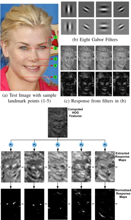
(a) Test Image with sample landmark points (1-5)

(b) Eight Gabor Filters

(c) Response from filters in (b)

P1 P2 P3 P4 P5

Computed HOG Features

Extracted Response

Maps

Normalized Response Maps

(d) Overview of Response Map Based Texture Model. After comput-ing HOG features for test image in (a), we convolve them with the discriminatively pre-trained filters (P1, . . . , P5) for each landmark. The responses are then normalized using a simple logistic function so that the values lie between 0 and 1. These normalized responses form the bases for the proposed response map based texture model.

Fig. 1: Background and overview of the proposed response map based texture model. In the following SectionII, we will show that these normalized response maps can be modeled and reconstructed accurately using a very small number of parameters.

illumination and expressions. In essence, the standard CLM frame-work follows a part-based approach in that the face is represented by a set of cropped image patches. A local detector (referred to as the ’patch-expert’) is trained for each landmark, using an off-the-shelf linear SVM and a large number of positive and negative patches [26]. Now, given a new face image, these patch-experts are used to perform an exhaustive local search around the initial shape estimate. As a result, a response map for each landmark point is generated which provides a likelihood of that landmark point being at a particular position in the given image. These response maps are then efficiently used to drive a simple Gauss-Newton method based optimization [25].

the discriminative training procedure of the patch-experts, and can themselves be represented by a small set of parameters. Hence, in this work, we propose to construct a novel texture model for robust face alignment based on these response maps. In prior work in computer vision, texture models are typically constructed by filtering the image using a set of pre-defined generic filters (e.g. difference of Gaussian, generative filters [11] or Gabor filters [19]1). Instead, we propose to construct a texture model by filtering the image with a set of filters, each of which have been discriminatively trained to localize a particular landmark point. The output of this filtering process is a sparse response map which can be then used to construct a robust texture model (to the best of our knowledge, this is the first time that the response maps generated via discriminatively learned filters are used to construct a texture model). In Figure 1, we give the overview of the proposed texture model. Within this proposed discriminative image filtering framework:

• We formulate a part-based approach and propose a

discrimi-native face alignment technique which uses the response map based texture model.

• We formulate a holistic approach by combining the proposed discriminative image filtering with generative deformable face models (i.e. AAM). This results in a hybrid discrimina-tive/generative face alignment framework in that the actual texture model is discriminative and the alignment method is generative in nature.

• We show that the proposed framework outperforms state-of-the-art methods (the CLM based RLMS [25] and the tree-based method [29]) convincingly. We release our code (See Supplementary Material) and the pre-trained models for research purposes.

II. MOTIVATION FORDISCRIMINATIVEIMAGEFILTERING

As stated earlier in SectionI, the main advantage of the standard CLM framework [25] over the AAMs [2] is the use of response maps to drive its optimization procedure, thereby decoupling the optimization procedure from the variations in facial texture induced by changes in identity, expressions, pose and illumination. Therefore, unlike the AAM optimization methods that suffer from the problem of lack of generalizability, mainly due to the texture model they use, the CLM optimization methods easily bypass these problems by working with the response maps instead of the actual facial appearance. However, one of the shortcomings of the standard CLM framework is that it does not fully exploit the true representative power of the response maps. In particular, in the CLM fitting objective function of [25], the optimization is performed over only the shape model parameters, and the response maps are used only indirectly in computing the weights for the non-parametric Gaussian mixture model that governs the possible landmark locations.

Therefore, in this paper, we make a case for a more direct use of the information provided by the response maps in the fitting procedure. This is motivated mainly due to the realization that: Firstly, each of these discriminatively trained filters (i.e. the patch experts) is tailored for a particular landmark point and can provide sparse filter response (or confidence) maps. Secondly, since invariance to external elements (like identity, pose, illumination and expressions that makes generic face fitting a very challenging task) is intrinsic to the response maps, a dictionary of response maps (controlled by a small set of parameters) can

1_{The experiments in [19] show that the methodology is only suitable} for person-specific scenario for the case of unseen illumination.

be easily created and used very accurately to reconstruct unseen response maps. As a result, a dictionary of response maps can be very efficiently used to replace the raw pixel value based texture model. This results in a non-rigid face alignment framework capable of handling the challengingin the wild scenario.

In this section, we empirically test the generalization capability of the proposed response map based texture model and compare it to the standard facial appearance based (i.e. pixel value based) texture model. For this purpose, we train two separate texture models based on the pixel values and the response map values, respectively, using the images from Multi-PIE database [14] only. We then reconstruct instances from unseen test images belonging to the Multi-PIE [14] and LFPW [4] databases. This highlight some highly desirable properties of the response maps and its texture model which include:distinct signatureof some landmark points,sparsity, compactnessandgeneralization capability.

See Appendix A in the supplementary material for details on the experimental setup. For training the pixel value based texture model, all the training images were similarity normal-ized [26], [25] and 31×31 patches were extracted around each landmark point. Let us assume we have a training set of image patches {Aij}Tj=1 for each landmark point i. A simple way to model the appearance of the patches for the ith landmark is to vectorize the training set of patches, stack them in a matrix Xi= [vec(Ai

1), . . . ,vec(AiT)] and use PCA to decompose into Xi≈ZiHi+MiwhereZi is the matrix that contains the PCA bases, Mi= [mi. . .mi] = 1

NXi11

T _{is a matrix that contains}

the mean vectormiin each column, andHi=ZTi(Xi−Mi)are the parameters for the training set of patches (i.e., the projection to the bases). Now, given a testing sample (i.e. a new unseen patch), it can be reconstructed by a small set of parametershtestthat are computed by a simple projections on the PCA basisZi.

For training the response map based texture model, all the 31×31 training patches (extracted above around each landmark point) were convolved with respective patch-experts (learned using the mentioned Multi-PIE training set) to generate training set of 31×31 response maps. Following the similar modeling procedure as above, each of the response maps were vectorized, stacked in a matrix and PCA was applied to compute the PCA basis. Now, given a testing sample (i.e. a new unseen response map), it can be reconstructed by a small set of parameters by just a simple projections on the response map PCA basis. An illustrative example on how effectively a response map can be reconstructed, as compared to the pixel value based image patch, by a very small number of PCA components (for example, the top 5 PCA components in this case) is shown in Figure2.

Figure3(a) shows the average reconstruction error for the patch around the left eye corner (i.e. landmark number 5 in Figure2) for Multi-PIE and in-the-wild LFPW test set using up to the top 20 PCA components of both the pixel value based and the response map based texture model. The average reconstruction error is computed as the mean-squared error between the ground-truth and the reconstructed patch. Further, in Figure3(b), we show average reconstruction error for the patch around all 66 landmark points for both the testing sets using top 5 PCA components of both the texture models.

1

2

3

6

4

5

7

8

(a)Sample LFPW Test Image

1. 2. 3. 4. 5. 6. 7. 8.

(b)Pixel Value Based Texture Model

1. 2. 3. 4. 5. 6. 7. 8.

(c)Response Map Based Texture Model

Fig. 2: Pixel Value based vs. Response Map based texture model: (a) Sample test image from LFPW with relevant landmarks labelled 1–8. (b) For landmarks 1–8: First row shows the extracted image patches. Second row shows the reconstructed image patches generated by the top 5 PCA components of each landmark’s pixel value based texture model. (c) For landmarks 1–8: First row shows the extracted response maps. Second row shows the reconstructed response maps generated by the top 5 PCA components of each landmark’s response map based texture model.

1 5 10 15 20 0

5 10 15 20 25 30 35 40

Number of Principal Components

Average Reconstruction Error

(Average MSE)

P−Model on LFPW Test Set P−Model on MultiPIE Test Set R−Model on LFPW Test Set R−Model on MultiPIE Test Set

1 66 1 66 1 66 1 66 0

3 6 9 12 15 18 21

Average Reconstruction Error

(Average MSE)

P−Model on MultiPIE Test Set P−Model on LFPW Test Set R−Model on MultiPIE Test Set R−Model on LFPW Test Set

Landmarks Landmarks Landmarks

Landmarks

(a) (b)

Fig. 3: Pixel Value based (P-Model) vs. Response Map based texture model (R-Model). (a) For the patch around Left Eye Corner, using upto top 20 PCA components. (b) For all landmark points, using top 5 PCA components.

quality as it drastically reduces the candidate locations for each landmark point. Having said that, the two most important qualities of the response map based texture model are its generalization capability and compactness. Notice the quality of reconstructed response maps for the Multi-PIE test set, but more importantly for the LFPW test set. The response map based texture model is able to generalize easily to the unseen response maps obtained from the LFPW test set, across all the landmark points. On the other-hand, we see a sharp rise in the reconstruction error for the LFPW test set obtained by the pixel value based texture model. Also, the excellent level of generalization obtained by the response map based texture model comes hand-in-hand with its compactness. As shown in Figure3(a), a stable reconstruction accuracy is obtained by using as few as the top 5 PCA components making the response map based texture model highly suitable for fast and accurate face alignment optimization strategies. Therefore, in the following sections, we propose the part-based and the holistic approaches that use the novel response map based texture model efficiently for generic face alignment under uncontrolled natural settings.

III. THEPART-BASEDAPPROACH A. Background

In the part-based model representation, the model setup isM=

{S,D}where S is the shape model and Dis the set of patch-experts. The 3D shape model of CLMs can be described as:

s(p) =sR(s0+Φsq) +t, (1)

parameterized by p = [s,R,t,q], where s, R (computed via pitchrx, yawryand rollrz) andt= [tx;ty; 0]control the rigid scale, 3D rotation and translation respectively, whileq controls the non-rigid variations of the shape.Dis a set of patch-experts for detection of nparts and is represented as D={wi, bi}ni=1, wherewi, biis the linear filter for theithlandmark point of the face (e.g., eye-corner detector).

The probability of alignment of a particular landmark point at a specific location xi in the given image Ican be modeled by using a simple logistic function [26], [25], [3]:

p(li= 1|x,I) =

1

1 +e[dCi(x;I)+c], (2) wherecis the logistic function intercept anddis the regression coefficient. The classifierCi(x;I)distinguishes between the align-ment/misalignment for a landmark location xi. We use Linear SVM for training the patch experts as:

Ci(x;I) =w|iP(F(x;I)) +bi (3)

where wi stands for gain and bi indicates bias, F(xi;I) is the vectorized feature vector extracted from the image patch centered atxi, and the functionPperforms normalization so that the result will have the property of zero mean and unit variance.

In the CLMs, the objective is to create a shape model from the parameterspsuch that the positions of the created model on the image correspond to well-aligned parts. In probabilistic terms, we want to find the shapes(p)by solving the following:

p= arg max

p p(s(p)| {l1= 1, . . . , ln= 1},I) = arg max

p p(p)p({l1= 1, . . . , ln= 1} |s(p),I)

= arg max p p(p)

n

Y

i=1

p(li= 1|xi(p),I).

(4)

B. Discriminative Fitting of Response Maps (DFRM)

Instead of maximizing the probability of a reconstructed shape [25], the alignment objective of the proposed part-based approach is to directly find shape model parameters that maximize the probability of all the landmark points being aligned. For this purpose, we propose to follow a discriminative regression based approach for estimating the required shape model parameters p. That is, we propose to find a mapping from the response map estimate of shape perturbations to shape parameter updates.

In particular, let us assume that in the training set we introduce a perturbation∆pand compute the response map in aw×w win-dow centered around each of the perturbed landmark points, repre-sented byAi(∆p) = [p(li= 1|x+xi(∆p)]. Then, from these responses obtained from the perturbed shapes{Ai(∆p)}n

i=1, we want to learn a functionf such thatf({Ai(∆p)}n

i=1) = ∆p. We call this methodDiscriminative Fitting of Response Maps (DFRM). Overall, the training procedure for the DFRM method has two main steps. In the first step, the goal is to train a dictionary for response map approximations. The second step involves iteratively learning the parameter update model which is achieved by a modified boosting procedure.

1) Training Part-Based Response Map Model: In this section, the goal is to build a part-based response map texture model, i.e. a dictionary of response maps, that can be used for representing any instance of an unseen response map. We aim to train a separate dictionary for the response maps obtained from each of the dis-criminatively trained patch-experts inD(3). In other words, each part-based response map texture model representsAi(∆p)using a small number of parameters. Let us assume we have a training set of response maps {Ai(∆pj)}T

j=1 for each landmark pointi with various perturbations (including no perturbation, as well). The simplest way to learn the dictionary for the i-th landmark point is to vectorize the training set of response maps and arrange them in a matrixXi= [vec(Ai(∆p1)), . . . ,vec(Ai(∆pT))]. As we motivated in Section II, we decompose Xi ≈ZiHi+Mi, whereHi= [hi(∆p1). . .hi(∆pT)]. Then, instead of finding a regression function from the perturbed responses{Ai(∆p)}n

i=1, we aim at finding a function from the low-dimensional weight vectors {hi(∆p)}n

i=1 to the update of the 3D shape model parameters∆p.

As we motivated in SectionII, extraction of the corresponding weight vectorhican be performed efficiently by a simple projec-tion on the PCA basis. An illustrative example of how effectively a response map can be reconstructed by a small number of PCA components (for example, top 5 PCA components) is shown in Figure2. We refer to this dictionary as thePart-Based Response Map Modelrepresented by:

RP ={M,V}:M={mi}ni=1andV={Zi}

n i=1 (5)

where, mi and Zi are the mean vector and PCA basis, respec-tively, obtained for each of the nlandmark points.

2) Training DFRM Update Model: Given a set ofN training imagesIand the set of corresponding shapesS, the goal is to iter-atively model the relationship between the joint low-dimensional projection of the response maps, obtained from the part-based response map modelRP, and the shape model parameters update (∆p). For this, we propose to use a modified boosting procedure in that we uniformly sample the 3D shape model parameter space, which controls all of the landmark positions simultaneously, within a pre-defined range around the ground truth parameters pg (1), and iteratively model the relationship between the joint low-dimensional projection of the response maps at the current sampled shape (represented bytth

sampled shape parameterpt)

and the shape model parameter update∆p(∆p=pg−pt). For the experiments in this paper, the predefined range is set to±15 pixels for translation,±10◦for rotation,±0.1for scaling and1.5 standard deviation (based on the available training set) for the non-rigid parameters (q). The step-by-step training procedure is as follow:

Algorithm 1: Training DFRM Update Model Require: PDM (1),I,S,RP (5).

Get initial shape parameters sample setP(1)_(6). 1

Get initial joint low-dimensional projection setχ(1)(7). 2

Generate training set for first iterationT(1)_. 3

fori= 1→ηdo 4

Compute the weak learnerF(i) _usingT(i)_. 5

PropagateT(i)_throughF(i)_{to generateT}(i) new. 6

Eliminate converged samples inTnew(i) to generateT(i+1). 7

ifT(i+1)_{is emptythen} 8

All training samples converged.Stop Training. 9

else 10

Get new shape parameters sample set (6) from images 11

whose samples are eliminated in Step 7.

Get new joint low-dimensional projection set (7) for the 12

samples generated in Step 11.

Generate newreplacementtraining setTrep(i). 13

forj= 1→(i−1)do 14

PropagateTrep(i) throughF(j). 15

Eliminate converged samples inTrep(i). 16

UpdateT(i+1)_{← {T}(i+1)_,T(i) rep} 17

Output: DFRM Update ModelU (10)

Let T be the number of shape parameters sampled from the shapes inS, such that the initial sampled shape parameter set is represented byP(1)

:

P(1)

={p(1)_j }T

j=1 and ψ(1)={∆p (1) j }

T

j=1 (6)

‘1’ in the superscript represents the initial set (first iteration). Next, extract the response maps for the shape represented by each of the sampled shape parameters in P(1) _{and compute} the low-dimensional projection usingRP. Then, concatenate the projections to generate a joint low-dimensional projection vector c(∆p(1)j ) = [h

T 1(∆p

(1) j ), . . . ,h

T n(∆p

(1) j )]

T

, one per sampled shape, such that:

χ(1)={c(∆p(1)_j )}T

j=1 (7)

where, χ(1)

represents the initial set of joint low-dimensional projections obtained from the training set. Now, with the training setT(1)_={χ(1)_{, ψ}(1)_}

, we learn the parameter update function for the first iteration i.e. a weak learnerF(1)

:

F(1)

:ψ(1)←χ(1) (8)

For this, any regression method can be employed in our frame-work. In this paper, we have chosen a simple Linear Support Vector Regression (SVR) [15] for each of the shape parameters. In total, we used 16 shape parameters : 6 global shape parameters (representing the six degrees of freedom corresponding to the 3D rigid transformation), and the top 10 local shape parameters (represented by q(1) corresponding to the 3D non-rigid shape variations). Structured regression based approaches can also be employed but we opted to show the power of our method with a simple regression framework.

Next, after learning F(1)

, we propagate all the samples from

T(1)

throughF(1)

to generateT1

the predicted shape and the ground truth shape is less than a threshold (for example, set to 2 pixels in this paper).

Now, in order to replace these eliminatedconverged samples, we generate a new set of samples (6)(7) from the same images inI

whose samples converged in the first iteration. We propagate this new sample set throughF1

and eliminate the converged samples to generate an additionalreplacementtraining set for the second iterationTrep. The training set for the second iteration is updated:(2)

T(2)← {T(2),Trep(2)} (9)

and the parameter update function for the second iteration is learned i.e. a weak learner F(2)

. The sample elimination and replacement procedure for every iteration has two-fold benefits. Firstly, it plays an important role in insuring that the progressive parameter update functions are trained on the tougher samples that have not converged in the previous iterations. And secondly, it helps in regularizing the learning procedure by correcting the samples that diverged in the previous iterations due to overfitting. The above training procedure is repeated iteratively until all the training samples have converged or the maximum number of desired training iterations (η) have been reached. The resulting DFRM update modelU is a set of weak learners:

U={F(1), . . . ,F(η)} (10) The training procedure is outlined in Algorithm1.

3) Alignment Procedure:Given the test imageItest, the param-eter update model U is used to compute the additive parameter update ∆piteratively. Theefficacy of alignment is measured as the alignment score that is computed for each iteration by simply adding the responses (i.e. the probability values) at the landmark locations estimated by the current shape estimate of that iteration. The final aligned shape is the shape with the highest alignment score. The alignment procedure is outlined in Algorithm2.

Algorithm 2: DFRM Alignment Procedure Require:Itestandsinitial

Computeptest(1) fromsinitial 1

Best= 0;

2

fori= 1→ηdo 3

Extract response maps forptestand compute the joint 4

low-dimensional projection (ctest)

∆p=Fi_(c test) 5

ptest←ptest+ ∆p 6

ComputeScoreforptest 7

ifScore>Bestthen 8

pf inal=ptest 9

Best=Score

10

Computestestfrompf inal(Eqn.1) 11

Output: Final Shape (stest)

IV. THEHOLISTICAPPROACH A. Background

The most well known generative holistic non-rigid face align-ment method is the Active Appearance Model [6], [2]. An AAM is fully defined by the triplet A = {S,T, W(x;ps)} where

S = {s0,Φs} and T = {t0,Φt} are the shape and texture models, whileW is a function that defines the motion model (e.g. piece-wise affine warps or thin-plate splines [2], [1]). The problem of fitting the modelAto a vectorized test imaget(originated from an imageI) is formulated as:

{po,co}= arg min p,c

t(W(x;p))−t0−Φtc

2

. (11)

Gauss-Newton gradient descent is the standard choice for solving (11). Please see [2] for details.

Mean Shape _{Warped Filter Responses}

Filter Responses

Fig. 4: The Holistic Response Map Based Texture Model.

B. Generative Fitting of Response Maps (GFRM)

The proposed holistic approach that relies on the response map based texture model is akin to the AAM framework [6], [2] in that it uses the 2D shape model and the motion model defined via warping function W. However, unlike the AAM framework that uses the facial appearance to drive the alignment procedure, the proposed holistic approach uses the response maps obtained from the discriminatively trained patch-experts. Here, the motion model defines how, given the shape, the corresponding response maps should be warped into the canonical reference frame (i.e. the mean shape). In this paper, we use the Piecewise Affine Warping [6], [2] method to generate these shape-free response maps.

The model setup for the holistic approach is{D,S, W}, where

Dis a set of patch-experts, S is the 2D shape model and W is the motion model. The 2D shape modelS is parameterized by p= [s, r, tx, ty,q], where,s, r, tx and tyare the global scaling, rotation and translations respectively, and

s=s0+Φsq (12)

where, s0 is the mean shape andΦs is the shape basis learned from a set of training shapes by applying PCA, andqis the non-rigid shape parameter vector.

Let us assume we have a training imageIand the corresponding 2D shapes, we compute the response maps{A1, . . . ,An}where

Nis the number of landmark points. Next, we generate the shape-free response maps Ai(W(x;p)) n

i=1 i.e. warp the response maps to the mean shape. The response map based texture vector tIis generated by vectorizing the shape-free response maps and

stacking them together i.e.

tI=

vec(A1(W(x;p)));. . .;vec(An(W(x;p)))

(13)

The whole procedure is summarized in Figure4. Let us assume we haveMtraining images, then the holistic response map texture model is obtained by simply applying PCA to a set of shape-free response map based texture vectorsti M_i=1 as

t=t0+Φtc (14)

where RH = {t0,Φt}is the holistically trained response map texture model, t0 is the mean shape-free response map texture vector andΦt = [Φ1. . .ΦK] is the texture basis matrix repre-sented by a set of Kknown response map texture variationsΦ. As a result, the complete model setup for the proposed holistic approach is{S,D, W,RH}.

patch-expertsD(3) toI, represented bytI(13), and the response

maps approximations synthesized via holistic response map tex-ture modelRH with respect to the model parameters:

n

pI,cI

o

= arg min

p,c ||tI−t0−Φtc||

2

. (15)

This optimization can be solved very efficiently using the inverse compositional algorithms [2] which is a variation of the Gauss-Newton optimization procedure. Within this framework, we focus mainly on the project-out algorithm and its alternating extension for the sake of computational efficiency.

1) Project-out method:In the project-out method, the optimiza-tion is formulated such that the shape model parameters p are found by the non-linear optimization in the subspace orthogonal to the texture basisΦt, thereby, ignoring the texture variation. In particular, the following optimization problem is solved:

{po}= arg min p

tI−t0

2

span(Φt)⊥. (16)

See Appendix B in the supplementary material for details. 2) Alternating method: The project-out optimization procedure described above is extremely fast, but has been shown to not be robust especially for the case of considerable texture variation [13]. Unfortunately, texture variation coincides with the in-the-wild setting assumed in this work. An alternative would be to simultaneously optimize shape and texture but this is extremely slow [13]. Fortunately, an alternative option exists via optimizing using an alternating optimization strategy. Suppose that the shape parameters are fixed. Then an update for the response map based texture model parameters can be readily obtained from ∆c = ΦTt(tI−t0)andc←c+ ∆c. Oncechas been updated, one can compute the reconstructed response maps fromtrec=t0+Φtc. The shape parameters can be updated by solving the following Lukas-Kanade problem:

pI= arg min

p ||tI−trec||

2

. (17)

See Appendix B in the supplementary material for details.

V. EXPERIMENTS ANDDISCUSSION

We conducted generic non-rigid face alignment experiments on the controlled and the uncontrolled (a.k.a. wild) databases. For controlled settings, we use Multi-PIE [14] database. For uncontrolled settings, we use LFPW [4], Helen [17] and AFW [29] databases. For all experiments, we consider the independent model (p1050) of the tree-based method [29], released by the authors, as the baseline for comparison. For the multi-view variant of the proposed approach, the pose range of ±30◦in yaw direction is divided into three view-based models, with each covering −30◦ to −15◦,−15◦to15◦, and15◦to 30◦ in yaw directions. Other non-frontal poses have been excluded for the lack of ground-truth annotations. See Appendix C in the supplementary material for a step-by-step description to train robust patch-experts used for the following experiments.

A. Overview of Results

We test the performance of the proposed DFRM (Section

III-B), GFRM-PO (SectionIV-B) and GFRM-Alternating (Section

IV-B) methods against the existing state-of-the-art RLMS [25] method and the tree-based method [29]. Since the main focus of this paper is on in-the-wild generic face alignment, we also compare the performance of the proposed framework with the very recently proposed Supervised Descent Method (SDM) [27] on three very challenging in-the-wild databases. Note that [25] [27] have not released their training code. Therefore, in order to perform a fair comparison with RLMS and SDM, we developed

our own implementations and trained our own models using exactly the same data as the other methods proposed in this paper. Furthermore, thanks to the authors of [29] who made both the training and testing code available for their algorithm, we used their code for training the tree-based models. We have to highlight once more that all the algorithms have been trained and tested on the same data and using the same features. Finally, even though we experimented with methodologies such as [19] that use generic filters, these methodologies did not work well in generic alignment scenarios, which is in line to the findings of [19].

• The Multi-PIE experiment focuses on accessing the

perfor-mance with combined identity, pose, expression and illumi-nation variation. Overall, the GFRM-Alternating method and the DFRM method show equally promising results over the state-of-the-arts RLMS [25] and the tree-based method [29].

• LFPW, Helen and AFW experiments further verify the gen-eralization capability of the proposed response map texture model based framework to handle challenging uncontrolled natural variations in that it outperforms the state-of-the-art RLMS [25] and tree-based method [29] convincingly. On these wild databases, the results show that GFRM-Alternating is again the best performing method followed by the DFRM and GFRM-PO method. The performance of DFRM is comparable to SDM [27].

• The results on LFPW, Helen and AFW database also

vali-date one of the main motivations behind the proposed face alignment framework i.e. the response maps extracted from an unseen image can be very accurately represented by a small set of parameters and are well suited for the task of generic face alignment under uncontrolled natural settings.

B. Multi-PIE Database Experiments

For this experiment, images of all 346 subjects, with all six expressions at frontal and non-frontal poses at various illumination conditions are used. The training set consisted of roughly 8300 images which included the subjects 001-170 at poses 051, 050, 140, 041 and 130 with all six expressions at frontal illumination and one other randomly selected illumination condition. The multi-view RLMS-MPIE refers to the method trained using the HOG feature based patch experts and the RLMS alignment method (Section III-A). The multi-view DFRM-MPIE refers to the method trained using the HOG feature based patch experts and the proposed DFRM alignment method (SectionIII-B2). The multi-view GFRM-PO-MPIE refers to the method trained using the HOG feature based patch experts and the proposed GFRM-PO alignment method (SectionIV-B1). The multi-view GFRM-Alt-MPIE refers to the method trained using the HOG feature based patch experts and the proposed GFRM-Alternating alignment method (Section IV-B2). For the tree-based method [29], we trained the tree-based model p204-MPIE that shares the patch templates across the neighboring viewpoints and is equivalent to the multi-view approach adopted for other alignment methods, using exactly the same training data for a fair comparison.

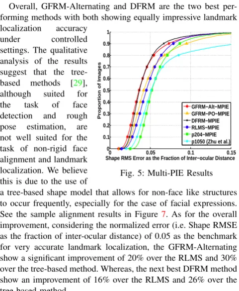
Overall, GFRM-Alternating and DFRM are the two best per-forming methods with both showing equally impressive landmark localization accuracy

under controlled settings. The qualitative analysis of the results suggest that the tree-based methods [29], although suited for the task of face detection and rough pose estimation, are not well suited for the task of non-rigid face alignment and landmark localization. We believe this is due to the use of

0 0.05 0.1 0.15

0 0.1 0.2 0.3 0.4 0.5 0.6 0.7 0.8 0.9 1

Shape RMS Error as the Fraction of Inter−ocular Distance

Proportion of Images

GFRM−Alt−MPIE GFRM−PO−MPIE DFRM−MPIE RLMS−MPIE p204−MPIE p1050 (Zhu et al.)

Fig. 5: Multi-PIE Results

a tree-based shape model that allows for non-face like structures to occur frequently, especially for the case of facial expressions. See the sample alignment results in Figure 7. As for the overall improvement, considering the normalized error (i.e. Shape RMSE as the fraction of inter-ocular distance) of 0.05 as the benchmark for very accurate landmark localization, the GFRM-Alternating show a significant improvement of 20% over the RLMS and 30% over the tree-based method. Whereas, the next best DFRM method show an improvement of 16% over the RLMS and 26% over the tree-based method.

C. Wild Database Experiments

To further test the ability of the proposed response map tex-ture model based framework to handle unseen and uncontrolled variations, we conduct experiments using three databases that presents the challenge ofwildnatural settings. The Labeled Face Parts in the Wild (LFPW) database [4] consist of the URLs to 1100 training and 300 test images that can be downloaded from internet. All of these images were captured in the wild and contain large variations in pose, illumination, expression and occlusion. We were able to download only 813 training images and 224 test images because some of the URLs are no longer valid. These images were manually annotated with 66 landmark point locations to generate the LFPW ground-truth annotations. On the other hand, the recently released Helen database [17] consist of 2000 training images and 330 test images. All of these images are collected from Flickr and present the challenge of being captured under completely natural real-world settings. From this, we manually annotated 890 training images and the entire test set of 330 images with 66 landmark point locations to generate the Helen ground-truth annotations. In addition, we used the extremely challenging annotated faces in-the-wild (AFW) database [29] to test the performance of the proposed methods on a completely unseen in-the-wild testset. The AFW test set consisted of 205 images with a total of 468 faces that were manually annotated with 66 landmark point locations to generate AFW ground-truth annotations.

To generate the wild training set, we augmented the Multi-PIE training set (used in SectionV-B) with the LFPW and Helen training sets. The models trained using this wild training set are referred as DFRM-Wild, GFRM-PO-Wild, GFRM-Alt-Wild, RLMS-Wild and p204-Wild. In addition, we also compare the performance of the proposed response-map texture model based framework to the Supervised Descent Method (SDM) [27]. For this, we trained both the single-view SDM (as originally proposed in [27]) and the multi-view SDM. SDM-Singleview-Wild refers

to the single-view SDM trained using the HOG features and the wildtraining set. SDM-Wild refers to the multi-view SDM trained using the HOG features and thewild training set.

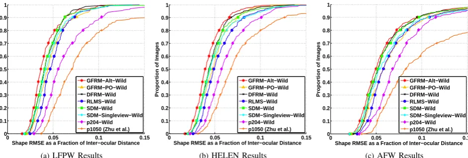
These were then used to perform non-rigid face alignment on the LFPW, Helen and AFW test sets and the results are reported in Figure 6. From these results, we can clearly see the dominance of the proposed DFRM, PO and GFRM-Alternating methods over the RLMS and the equivalent tree-based methodp204. The performance of multi-view SDM approach is comparable to that of DFRM. Considering the normalized error of 0.05 as the benchmark for very accurate landmark localization, GFRM-Alternating shows significant overall improvement of 20% over the RLMS and 39% over the tree-based method. Whereas, the DFRM method shows an overall improvement of 14.5% over the RLMS and 33% over the tree-based method.

GFRM-Alternating method is consistently the best performing method. Our results show that the proposed generative and dis-criminative methods outperform other state-of-the-art approaches under the generic face alignment scenario. Moreover, they also demonstrate the ability to handle the challenging variations present in thewilddatabases (pose, illumination, facial hair, glasses and ethnicity). This result validates the main motivation behind the proposed framework (i.e. the response maps extracted from an unseen image can be very accurately represented by a small set of parameters and are suited for the task of generic face alignment). See the sample alignment results in Figure7.

VI. CONCLUSION

In this paper, we proposed a new response map texture model based generic face alignment framework that shows state-of-the-art results in the wild. For this, firstly, we empirically validated the superiority of the response map based texture model over the pixel value based texture model. Secondly, within this framework, we proposed a part-based alignment method (i.e. DFRM) and two holistic model based alignment methods (i.e. GFRM-PO and GFRM-Alternating) that can handle challenging in-the-wild conditions. Overall, the proposed methods are highly efficient and real-time capable.

The current MATLAB implementation of the multi-view GFRM-Alternating, GFRM-PO and DFRM methods take 4 sec/image, 1 sec/image, and 1 sec/image, respectively, on an Intel Xeon 3.60 GHz processor. Moreover, the current C/CUDA implementation of DFRM method runs at 30-45 FPS on an Intel Xeon 3.60 GHz processor with NVIDIA GeForce GTS 450 graphic card (192 Cores). In this implementation, the response map for each landmark point is computed in parallel using CUDA, allowing the DFRM fitting to perform in real-time. On the other hand, the GFRM-Alternating method requires the Hessian and its inverse to be computed at each iteration. Therefore, making a real-time GFRM implementation is not straight-forward and is left as future work. See supplementary material for additional experimental results on benchmarking the accuracy fitting results (Appendix D), in-the-wild occluded images (Appendix E) and images under varying resolution (Appendix F).

Acknowledgment:The work of A. Asthana is funded by Marie Curie Fellowship under FP7-PEOPLE-2011-IIF Grant agreement no. 302836 (FER in the Wild). The work of S. Cheng and S. Zafeiriou is funded by the EPSRC project EP/J017787/1 (4D-FAB). The work of G. Tzimiropou-los is funded by the European Community 7th Framework Programme [FP7/2007-2013] under grant agreement no. 288235 (FROG).

REFERENCES

[1] B. Amberg, A. Blake, and T. Vetter. On compositional image alignment, with an application to active appearance models. In

0 0.05 0.1 0.15 0

0.1 0.2 0.3 0.4 0.5 0.6 0.7 0.8 0.9 1

Shape RMSE as a Fraction of Inter−ocular Distance

Proportion of Images

GFRM−Alt−Wild GFRM−PO−Wild DFRM−Wild RLMS−Wild SDM−Wild SDM−Singleview−Wild p204−Wild p1050 (Zhu et al.)

(a)LFPW Results

0 0.05 0.1 0.15

0 0.1 0.2 0.3 0.4 0.5 0.6 0.7 0.8 0.9 1

Shape RMSE as a Fraction of Inter−ocular Distance

Proportion of Images

GFRM−Alt−Wild GFRM−PO−Wild DFRM−Wild RLMS−Wild SDM−Wild SDM−Singleview−Wild p204−Wild p1050 (Zhu et al.)

(b)HELEN Results

0 0.05 0.1 0.15

0 0.1 0.2 0.3 0.4 0.5 0.6 0.7 0.8 0.9 1

Shape RMSE as a Fraction of Inter−ocular Distance

Proportion of Images

GFRM−Alt−Wild GFRM−PO−Wild DFRM−Wild RLMS−Wild SDM−Wild SDM−Singleview−Wild p204−Wild p1050 (Zhu et al.)

(c)AFW Results

Fig. 6: Experimental Results. See SectionV-Band SectionV-Cfor details.

Fig. 7: Sample Alignment Results (Column 1-3: Multi-PIE Results. Column 4-10: LFPW Results. Column 11-16: HELEN Results). Row 1: GFRM-Alternating Results. Row 2: DFRM Results. Row 3: GFRM-PO Results. Row 4: RLMS [25] Results. Row 5: p204 tree-based method [29] Results.

[2] S. Baker, R. Gross, and I. Matthews. Lucas-Kanade 20 years on: A unifying framework: Part 3. Technical report, RI, CMU, USA, 2003.

1,2,5,6

[3] T. Baltrusaitis, P. Robinson, and L. Morency. 3D constrained local model for rigid and non-rigid facial tracking. InCVPR, June 2012.

3

[4] P. N. Belhumeur, D. W. Jacobs, D. J. Kriegman, and N. Kumar. Localizing parts of faces using a consensus of exemplars. InCVPR, 2011.1,2,6,7

[5] X. Cao, Y. Wei, F. Wen, and J. Sun. Face alignment by explicit shape regression. InCVPR, 2012. 1

[6] T. Cootes, G. Edwards, and C. Taylor. Active Appearance Models. InECCV, 1998.5

[7] T. Cootes, C. Taylor, D. Cooper, and J. Graham. Active shape models - their training and applications.CVIU, 1995. 1

[8] T. F. Cootes, M. C. Ionita, C. Lindner, and P. Sauer. Robust and accurate shape model fitting using random forest regression voting.

InECCV (7), pages 278–291, 2012. 1

[9] D. Cristinacce and T. Cootes. Feature detection and tracking with constrained local models. InBMVC, 2006.1

[10] N. Dalal and B. Triggs. Histograms of oriented gradients for human detection. InCVPR, 2005.

[11] F. De la Torre, A. Collet, M. Quero, J. F. Cohn, and T. Kanade. Filtered component analysis to increase robustness to local minima in appearance models. InCVPR, pages 1–8, 2007.2

[12] G. Edwards, C. Taylor, and T. Cootes. Interpreting Face Images Using Active Appearance Models. InIEEE FG, 1998. 1

[13] R. Gross, I. Matthews, and S. Baker. Generic vs. person specific active appearance models.IMAVIS, 23(12):1080–1093, 2005.6

[14] R. Gross, I. Matthews, J. Cohn, T. Kanade, and S. Baker. Multi-PIE.

InIEEE FG, 2008. 2,6

[15] C. Ho and C. Lin. Large-scale linear support vector regression. Technical report, Technical report, NTU, 2012. 4

[16] H. T. Ho and R. Chellappa. Pose-invariant face recognition using markov random fields.IEEE TIP, 22(4):1573–1584, April 2013.1

[17] V. Le, J. Brandt, Z. Lin, L. D. Bourdev, and T. S. Huang. Interactive facial feature localization. InECCV (3), pages 679–692, 2012.6,7

[18] X. Liu. Generic face alignment using boosted appearance model. In

CVPR, pages 1–8, 2007.1

[19] S. Lucey, S. Sridharan, R. Navarathna, and A. B. Ashraf. Fourier lucas-kanade algorithm. IEEE T-PAMI, 35(6):1383–1396, 2013. 2,

6

[20] I. Matthews and S. Baker. Active Appearance Models Revisited.

IJCV, 60(2):135–164, Nov. 2004. 1

[21] T. C. Patrick Sauer and C. Taylor. Accurate regression procedures for active appearance models. InProc. BMVC, pages 30.1–30.11, 2011.1

[22] J. Saragih and R. Goecke. Iterative Error Bound Minimisation for AAM Alignment. InICPR, 2006. 1

[23] J. Saragih and R. Goecke. A Nonlinear Discriminative Approach to AAM Fitting. InICCV, 2007.1

[24] J. Saragih and R. Goecke. Learning AAM fitting through simulation.

Pattern Recognition, 42(11):2628–2636, Nov. 2009. 1

[25] J. Saragih, S. Lucey, and J. Cohn. Deformable model fitting by regularized landmark mean-shift. IJCV, 91(2):200–215, Jan. 2011.

1,2,3,4,6,8

[26] Y. Wang, S. Lucey, and J. Cohn. Enforcing convexity for improved alignment with constrained local models. InCVPR, June 2008. 1,

2,3

[27] Xuehan-Xiong and F. De la Torre. Supervised descent method and its application to face alignment. InCVPR, 2013. 6,7

[28] Y. Yang and D. Ramanan. Articulated pose estimation with flexible mixtures of parts. InCVPR, pages 1385–1392, 2011.