A two-fluid model for tissue growth within a
dynamic flow environment
R. D. O ’Dea1, S. L. Wa ter s2 and H. M. Byr ne1
1
School of Mathematical Sciences, University of Nottingham, University Park, Nottingham, NG7 2RD email:[email protected]
2
Mathematical Institute, 24-29 St Giles’, Oxford, OX1 3LB
(Received 26thMarch 2008 / Accepted in revised form 4thJuly 2008)
We study the growth of a tissue construct in a perfusion bioreactor, focussing on its response to the mechanical environment. The bioreactor system is modelled as a two-dimensional channel containing a tissue construct through which a flow of culture medium is driven. We employ a multiphase formulation of the type presented by Lemonet al.[37], restricted to two interacting fluid phases, representing a cell population (and attendant extracellular matrix) and culture medium, and employ the simplifying limit of large in-terphase viscous drag after Franks, Franks & King [21, 23].
The novel aspects of this study are: (i) the investigation of the effect of an imposed flow on the growth of the tissue construct, and (ii) the inclusion of a mechanotransduction mechanism regulating the response of the cells to the local mechanical environment. Specif-ically, we consider the response of the cells to their local density and the culture medium pressure. As such, this study forms the first step towards a general multiphase formulation that incorporates the effect of mechanotransduction on the growth and morphology of a tissue construct.
The model is analysed using analytic and numerical techniques, the results of which illustrate the potential use of the model to predict the dominant regulatory stimuli in a cell population.
1 Introduction
In vitro tissue engineering is the logical extension of transplant surgery and involves the growth of replacement tissue outside the body to alleviate the chronic shortage of tissue available from donors [15]. Significant research has been dedicated to the study of tissue engineering processes relevant to liver, skin, collagen (for cartilage/tendon replacement) and bone (see [15, 60] for interesting reviews) and progress has been made in a num-ber of areas. These include: maintenance of tissue-specific functions via mimicry of in vivo conditions through appropriate cell co-culture and/or three-dimensional spheroidal culture [3, 26, 28, 41, 55]; and understanding the influence of artificial scaffolds which provide mechanical support for construct growth and whose surface chemistry and pore size may be altered to encourage cell anchorage or increased population of the scaffold [30, 58, 65].
formation of a construct with viable, proliferating cells at its periphery but a necrotic core: early studies have shown that cellular spheroids of diameter greater than 1mm gen-erally develop a necrotic core [61]. Depending upon the application, engineered constructs must be relatively large to serve as grafts for tissue replacement; it is clear, therefore, that mass-transfer limitations represent challenges for in vitro tissue engineers [45]. To rectify this, bioreactors are widely used. A bioreactor is an advanced tissue culture appa-ratus which enables control of the culture environment. Nutrient supply and metabolite removal may be enhanced by using perfusion or circulation/mixing strategies; further-more, bioreactors allow monitoring and control of factors such as pH, and the provision of growth factors and other cell-signalling molecules.
As well as controlling the biochemical environment, many bioreactors are designed specifically to provide mechanical stimulation to cell cultures via, for instance, fluid shear stress or tensile or compressive forces applied either on the macroscale or via magnetic particles embedded in the cell membrane (see [8, 45] for a review). These stimuli are integrated into the cellular response via a process known asmechanotransduction. The importance of mechanical stimuli to tissue function is noted by many authors including Fung [24], who asserts that the correct function of organs is dependent on the level of internal stress. A great many “proof of principle” studies have illustrated the beneficial effect of mechanical conditioning on the structural and functional properties of engineered tissues; however, little is known about either the manner in which these forces should be applied for specific tissues or how these stimuli are interpreted by the cells [45]. It is clear, however, that the mechanical environment required for optimum growth will be peculiar to the tissue under consideration; bespoke bioreactors are therefore required to provide appropriate physical (and biochemical) cues for different tissue engineering applications. Mathematical modelling of tissue growth is a subject area which has received a great deal of attention; the clinical applications of such models are myriad. In particular, much work has been dedicated to modelling tumour growth [1], angiogenesis [9, 11], wound healing [59] and, more recently, in vitro tissue engineering processes [13, 14]. Within the context of tissue engineering, the goals of such models are to explain how observed tissue engineering problems arise, to suggest mechanisms to resolve them and, thereby, to predict optimal protocols for tissue growth. Furthermore, idealised tissue growth studies can provide insights useful in the design of bespoke bioreactor systems.
A variety of approaches has been used to model tissue growth. Discrete cellular au-tomata models are employed in, for example, [20, 49, 50], while in [31, 32] chemotaxis-based continuum models are exploited (see [40] for a review). Numerous studies have considered the effect of limited nutrient availability and/or the presence of inhibitors on tissue growth (e.g. in the context of tumour growth [5, 25, 42]; for a review see [1]). The stresses experienced by cells at the microscopic level are calculated in [29, 46, 62]; the influence of the cells’ mechanical environment on growth is considered by Roose [57] in the context of growth-induced stresses, and scaffold adhesion-guided behaviour is investigated by Powerset al.[52, 53].
model. Parameter estimation is achieved via comparison with experimental evidence. Three-dimensional fluid flow through porous scaffolds in a perfusion bioreactor is stud-ied by Porter et al. [51] in which a detailed model of a porous scaffold is obtained via micro-computed tomography imaging and the flow profile calculated using the Lattice-Boltzmann method. Relating simulation results to experimental results, it is concluded that a mean pore-surface shear stress of 5×10⁻⁵
Pa corresponds to increased cell prolif-eration and viability. Raimondiet al.[54] demonstrate that the material properties and cell viability of constructs resulting from perfusion shows a two-fold improvement com-pared to surface perfusion or static culture; computational modelling is used to quantify the fluid-dynamical environment at the microscopic level. Modelling of both cell growth and fluid flow within a three-dimensional scaffold in a perfusion bioreactor is considered by Colletti et al. [12]. The flow through the scaffold is governed by Brinkman’s equa-tion and nutrient distribuequa-tion is governed by a reacequa-tion-advecequa-tion-diffusion equaequa-tion. Cell growth is assumed to depend upon local nutrient availability via an ordinary differential equation.
In this paper, we present a continuum mathematical model relevant to tissue growth processes in a perfusion bioreactor. In contrast to the above analyses of perfusion bioreac-tors [12, 43, 51, 54], we employ a multiphase formulation after Lemonet al.[37], restricted to two interacting viscous fluid phases, representing a cell population and attendant ex-tracellular matrix (ECM) and a culture medium (fluid-based models for biological tissue growth have been widely exploited, especially in modelling tumour growth; see, for exam-ple, [6, 7, 21, 23]). We consider this model to be a first step towards a general multiphase formulation allowing examination of the effect of mechanotransduction on the growth and subsequent morphology of a tissue. Our continuum macroscale model allows explicit consideration of the complex interactions involved in tissue growth without considering the precise microscopic detail; however, the averaging process involved in deriving models of this type ensures that the terms present in the model equations arise from appropriate microscopic considerations. The derivation and analysis of multiphase models (for bio-logical and other applications) has been treated in great detail in the literature; see, for example, [2, 35, 44, 63], and for two phase flows [16–18].
The perfusion bioreactor under consideration is based upon that employed by El-Haj et al. (see, for example, [19]) which comprises a tissue construct within a culture medium-filled cylinder along which a flow is driven; however, the mathematical techniques and modelling approaches employed here are readily transferrable to other tissue culture systems. Our model accommodates mechanotransduction-affected cell proliferation, ECM deposition and cell death. Nutrient-limited growth is not considered since we assume that perfusion provides an abundant supply of nutrient. The investigation of the effect of the imposed flow on the response of the cell phase and the inclusion of a simple mechanotransduction mechanism are the novel aspects of this study.
these interfaces to transverse perturbations is investigated (§3.1). Numerical solutions are obtained for a diffuse one-dimensional cell population growing at a constant rate (§3.2) and in §4.1, corresponding two-dimensional numerical simulations are presented. Lastly, in§4.2 we extend the model by coupling the cells’ proliferative response to the local mechanical environment, allowing consideration of a simple mechanotransduction mechanism. A discussion of our model and its applications within a tissue engineering context are presented in§5, together with suggestions for future work.
2 A two phase model for tissue growth
We apply the general multiphase formulation given in [37] to develop a simple model relevant to tissue engineering processes. For brevity, we do not recapitulate the multiphase formulation here: the interested reader is directed to [17, 35, 37] for more details.
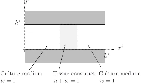
We consider the growth of a tissue construct within a nutrient-rich fluid culture medium and investigate the effect of an imposed flow on the response of the cells. We neglect the solid characteristics of the tissue construct (including, for instance, the presence of a scaffold) and employ a two-fluid model of the type presented in [4, 6, 17, 21, 23, 33]. This system is representative of tissue culture within a dynamic flow environment, for example, a perfusion-type bioreactor system. Our idealised perfusion bioreactor model is based upon that employed by El-Haj et al. and we represent this system as a two-dimensional channel containing a two phase mixture of interacting viscous fluids. A two-dimensional Cartesian geometry is chosen for simplicity; however, generalisation to a cylindrical geometry is straightforward. The cells and ECM are modelled as a single phase (henceforth denoted the “cell phase”); the second phase represents the culture medium. Perfusion is represented by an imposed flow of culture medium. In the following we will employ the term “tissue construct” to distinguish the region occupied by the interacting system of cell and culture medium phases from the remainder of the channel which contains only culture medium. At certain stages in this paper, the interface between the construct and the surrounding culture medium will be assumed to be sharp or diffuse to allow different analyses to be undertaken.
Tissue construct Culture medium Culture medium
w= 1
w= 1 n+w= 1
x∗ y∗
h∗
[image:4.612.186.425.473.615.2]L∗
Figure 1. An idealised model of a perfusion bioreactor as a two-dimensional channel of length
Nomenclature
n, w, s, θ Volume fraction of cell, culture medium, scaffold phases; porosity
p∗
w, p∗n, Σ∗n Culture medium and cell phase pressure; intraphase pressure (Nm−
2
)
S∗
n, Sw∗ Net material transfer rate into cell and culture medium phases (s−
1
)
σ∗n, σ∗w Stress tensor for the cell and culture medium phases (Nm−
2
)
u∗n, u∗w Velocity of cell and culture medium phases (ms−
1
)
F∗
wn, F∗nw Forces (per unit volume) between cell and culture medium phases (Nm−
3
)
x∗= (x∗, y∗) Spatial coordinate in horizontal and vertical directions (m)
t∗ Time (s)
Table 1. Nomenclature and units
A Cartesian coordinate systemx∗= (x∗, y∗) is chosen with corresponding coordinate directions (ˆx,yˆ) and the channel occupies 06x∗6L∗, 06y∗6h∗(see figure 1). In this paper, asterisks distinguish dimensional quantities from their dimensionless equivalents. We associate with each of the cell and culture medium phases a volume fraction, denoted nandw, respectively, and a volume-averaged velocity,u∗i = (ui∗, vi∗), pressure,p∗i, stress tensor, σ∗i and density, ρi (where i = n, w denotes variables associated with the cell and culture medium phases, respectively) and assume that these are functions ofx∗ and t∗, where t∗ represents time. Table 1 summarises the variables employed in the model, together with their units (where appropriate).
Assuming that each phase is incompressible with the same density, and neglecting inertial effects, we obtain the following governing equations (see [37]):
conservation of mass: ∂n
∂t∗ +∇ ∗·(nu∗
n) =Sn∗+D∗∇∗
2
n, (2.1)
∇∗·(nu∗
n+wu∗w) =Sn∗+Sw∗; (2.2)
conservation of momentum: ∇∗·(wσ∗
w) +F∗wn=0, (2.3)
∇∗·(nσ∗
n+wσ∗w) =0; (2.4)
no-voids: n+w= 1. (2.5)
In equations (2.1) and (2.2), S∗
n, Sw∗ are the net rates of material production for each phase and D∗ is the diffusion coefficient for the cell phase. In (2.3), F∗
wn represents the force exerted by the cell phase on the culture medium at the interface between these phases, and we assumeF∗
wn=−F∗nwas implied by (2.4). As in Drew [17], the influence of these interfaces, especially with respect to thermodynamic properties, is not considered; see Kolev [35] for a thorough discussion of these terms.
We remark that a diffusive term has been added to the mass conservation equation (2.1); whilst cells do exhibit random motion, the tissue growth and perfusion-induced flow fields are the dominant mechanisms leading to cell movement, with diffusive effects assumed to be negligible [22, 33]. However, we retain diffusive terms for numerical con-venience since they eliminate the moving boundaries between the tissue construct and culture medium, ensuring that we need not track explicitly the sharp interface which is evident whenD∗= 0.
interphase forces (F∗
ij), stress tensors (σ∗i) and material production rates (S∗i) which describe the behaviour of our system.
Following [4, 6, 37], we represent the interphase force as follows:
F∗
wn=p∗w∇∗w+k∗(u∗n−u∗w), (2.6)
wherein the pressure in the culture medium phase is denotedp∗
w, andk∗is the coefficient of interphase viscous drag, which we assume is constant. The pressure in the cell phase is related to that in the culture medium by the following relation:
p∗
n =p∗w+ Σ∗n, (2.7)
where Σ∗
n is a prescribedintraphase pressure resulting from interactionswithin the cell phase such as osmotic stresses or surface tension within cell membranes. Equation (2.7) will be employed to eliminate the cell phase pressure,p∗
n, from the governing equations and carries the tacit assumption that the interphase tractions are negligible. We do not specify a functional form for the intraphase pressure function, Σ∗
n, since in the analy-sis presented in this paper, we employ a lumped pressure field which encapsulates this function. Appropriate functional forms for intraphase pressures and interphase tractions are given in [6, 37]. Each of the phases are modelled as viscous fluids and the associated volume-averaged stress tensors are therefore
σ∗i =−p∗iI+µ∗i(∇∗u∗i +∇∗u∗iT) +λ∗i(∇∗·u∗i)I; i=n, w, (2.8)
where µ∗
i and λ∗i are the dynamic shear and bulk viscosity coefficients of the ith phase andIis the identity matrix. Functional forms for the material production terms S∗
i will
be chosen to reflect different physical processes at various points in this paper and we delay specification of appropriate boundary conditions until the derivation of a model in the limit of large interphase viscous drag.
We non-dimensionalise as follows:
x∗=L∗x, t∗= L ∗
U∗ w
t, u∗i =Uw∗ui, (p∗w,Σ∗n) = U ∗
wµ∗w
L∗ (pw,Σn), S ∗
i =
U∗ w
L∗Si, (2.9)
whereinU∗
w is a velocity scale which will be determined by the choice of pressure drop or upstream flux. A viscous scaling is employed for the culture medium and intraphase pressures (pw, Σn) since we assume that viscous effects dominate inertia in the momentum equations. In view of the non-dimensionalisationt∗ =L∗t/U∗
The dimensionless form of equations (2.1)–(2.4) is as follows:
∂n
∂t +∇ ·(nun) =Sn+D∇ 2
n, (2.10)
∇ ·(nun+wuw) =Sn+Sw, (2.11)
w∇pw+k(uw−un)− ∇ ·
w(∇uw+∇uTw) +γww(∇ ·uw)I
= 0, (2.12) ∇ ·−(pw+nΣn)I+µnn(∇un+∇uTn) +γnn(∇ ·un)I
+w(∇uw+∇uTw) +γww(∇ ·uw)I = 0, (2.13)
and equation (2.5) is used to eliminatew.
In equations (2.10)–(2.13), the dimensionless parameters D, µn, k, γw and γn are defined as follows:
D= D∗ U∗
wL∗
, µn = µ∗
n µ∗ w
, k=k∗L∗ 2 µ∗
w
, γw= λ∗
w µ∗
w
, γn= λ∗
n µ∗ w
, (2.14)
and the channel now occupies 06x61, 06y6h=h∗/L∗. The physical interpretation of the dimensionless diffusion coefficient (or inverse Peclet number)D, relative viscosity µn, and drag coefficientkis obvious. The parameterγidescribes the relative importance of the viscosity associated with the rate of change of volume of theith phase compared to that associated with fluid shear. It is usual to takeλ∗
i =−2µ∗i/3 (so that in equation (2.8), we have pi = −σi,kk/3; i = n, w) implying γw = −2/3 and γn = −2µ∗n/3µ∗w [21, 23, 33, 37]. We expectµ∗
n >µ∗wand therefore assumeγn6−2/3.
2.1 Large drag limit
By considering the Stokes drag due to water flowing past a spherical cell, Lubkin & Jack-son [39] estimated the drag coefficient as:k∗= 4.5×10⁷
N·m−4
·s. An appropriate length-scale for the system is the bioreactor length, and assuming that this is of the same order as the scaffold length, we chooseL∗ = 4×10⁻³m. Assuming that the culture medium viscosity is equal to that of water,µ∗
w= 1×10−
3N ·m−2
·s [36], the dimensionless drag coefficient may then be calculated from equation (2.14) to give:
k=k∗L∗ 2
µ∗ w
= 7.2×10⁵
. (2.15)
Motivated by this, we now consider the limit in which the interphase viscous drag is large (k≫1) and derive appropriate simplified versions of the governing equations and boundary conditions.
We consider a power series expansion of the dependent variables as follows:
n(x, t) =n0(x, t) +√1
kn1(x, t) + 1
kn2(x, t) +· · ·, (2.16)
with similar expansions forun,uw, pw and Σn; at leading order, equation (2.12) gives un0=uw0=u0so that we may associate with each phase a common velocity. Following [21, 23], we assume that each phase has the same material properties (γi =−2/3,µn = 1) and that at leading order the mass production termsSn0,Sw0are given by
in which km = (k∗mL∗)/Uw∗ represents the dimensionless rate of cell mitosis and ECM deposition (in the interests of brevity we henceforth refer to this as the “growth rate”), kd = (k∗dL∗)/Uw∗ represents the dimensionless rate of cell death and ECM degradation (which we will refer to as the “death rate”) andk∗
mandk∗d are the corresponding dimen-sional rates. In general, these will depend upon the cells’ mechanochemical environment (e.g.nutrient availability, growth factors, local cell density or stress) and in the following derivation we therefore allow spatio-temporal variation:km(x, t),kd(x, t).
Dropping the subscript notation for brevity, from (2.11)–(2.13), we obtain the following equations at leading order:
∇ ·u=kmn, (2.18)
∇p=∇2 u+1
3∇(∇ ·u), (2.19)
where the lumped pressure field,p, is related to pw0 viap=pw0+n0Σn0. Taking the divergence of equation (2.19) gives an expression for ∇2
(∇ ·u), which, on substitution into the Laplacian of (2.18), yields an equation for the pressure in terms of the cell volume fraction only. We may then restate our governing equations in the more natural form given in [21, 23]:
∂n
∂t +∇ ·(nu) = (km−kd)n+D∇
2n, (2.20)
∇2p= 4 3∇
2(k
mn), (2.21)
∇2
u=∇p−1
3∇(kmn). (2.22)
This model breaks down in a boundary layer of thickness O(1/√k) near the channel walls when intraphase viscous effects become important (see equation (2.12)); appropriate boundary conditions on the outer problem are given in Franks [21] as follows:
∂u
∂x =kmn− ∂v
∂y, v= 0, ∂n ∂y = 0,
∂p
∂y = 0, at y= 0, h, (2.23)
which imply slip along, but no-penetration of cells or culture medium throughy= 0, h. Axial boundary conditions which ensure that the tissue construct does not extend along the channel’s length and, additionally, set an axial pressure drop which drives a flow are as follows:
n = 0, pw=Pu, onx= 0, (2.24)
n = 0, pw=Pd, onx= 1, (2.25)
whereinPu andPd are the dimensionless up- and downstream pressures, related to the corresponding dimensional pressures via (Pu, Pd) = (Pu∗, Pd∗)L∗/(Uw∗µ∗w). In the following sections, we present solutions to the model equations (2.20)–(2.25) in various limits.
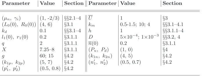
Parameter Value Section Parameter Value Section
(µn, γi) (1, -2/3) §§2.1–4 U 1 §3
(L0(0), R0(0)) (4, 6) §3.1 km 0.5-1.5; 10; 4 §§3.1–4.1
kd 0.1 §§3.1–4 h 1 §§3.1.1–4
l1(0), r1(0) 0.2 §3.1.1 D 5×10− 4
; 1×10⁻³
§§3.2, 4
q 2 §3.1.1 n(0) 0.2 §3.1.1
X 7.25–8 §3.1.1 (Pu, Pd) (1, 0) §4
g 60; 15 §4.2 (k1n, k2n) (4, 5) §4.2
(k1p, k2p) (5, 7) §4.2 (n′1, n′2) (0.5, 0.7) §4.2
(p′
[image:9.612.115.467.71.203.2]1, p′2) (0.5, 0.8) §4.2
Table 2. The (dimensionless) model parameters and values used in the numerical solutions together with the section(s) in which they are employed.
solutions for a diffuse cell population (D 6= 0) are presented and compared with the analytic solutions from§3.1. In§4.1, corresponding two-dimensional numerical solutions are presented. In§4.2, we further extend the model by postulating functional forms for the growth rate, km(x, t), which allow the influence of a range of mechanical stimuli on the growth response of the cells to be accommodated. We remark here that in all of the subsequent numerical simulations, the parameter values are selected to illustrate the behaviour of the model under a particular growth regime. The parameter values employed in each of the following sections are summarised in table 2.
3 One-dimensional growth
We now assume that the tissue undergoes one-dimensional growth parallel to thex-axis and that the associated pressure and velocity fields are functions ofx and t only. For mathematical convenience, we initially consider growth within a channel of semi-infinite length. In this case, equations (2.20)–(2.22) reduce to give
∂n ∂t +
∂
∂x(nu) = (km−kd)n+D ∂2
n
∂x2, (3.1)
∂2 p ∂x2 =
4km 3
∂2 n ∂x2,
∂2 u ∂x2 =
∂p ∂x −
km 3
∂n
∂x, (3.2a,b)
and we emphasise that we consider uniform growth, for whichkm andkd are constant. The axial boundary conditions presented in§2.1 require modification since the channel is now semi-infinite in extent. Integration of equation (3.2a) yields
p= 4km
3 n+α(t)x+β(t), (3.3)
whereα(t),β(t) are arbitrary functions of time; application of the boundary conditions p= Pu, n = 0 at x = 0,p = Pd, n = 0 as x→ ∞ indicates that we requireα = 0, β =Pu =Pd. A pressure drop-induced flow may therefore not be imposed; instead, we impose an upstream flow, U∗, corresponding to u(x= 0, t) =U, where U =U∗/U∗
w is
the dimensionless upstream flowspeed. In the following, we chooseU = 1, which sets the velocity scale to beU∗
w=U
∗
and we choosePu= 0 =Pd without loss of generality. We remark that the lengthscale, L∗, is now defined by our choice of growth rate according to k
m =km∗L∗/Uw∗, so that the lengthscale of interest is the distance travelled by a fluid particle over the growth timescale. Appropriate boundary conditions are
p= 0, n= 0, u= 1, at x= 0, (3.4)
p= 0, n= 0, ∂u
∂x = 0, as x→ ∞. (3.5)
Equation (3.3) (withα=β= 0) allows us to obtain a reduced model in terms of the cell volume fraction (n) and axial velocity (u) only (details omitted).
3.1 Sharp interface limit: D= 0
We now consider the regime in which the interfaces between the tissue construct and surrounding culture medium are sharp, corresponding to D = 0. The domain is then decomposed into three distinct regions by planar interfaces. We denote the interfacial positions byx =L(t), R(t), across which we impose continuity of velocity and normal stress:
[u]+−= 0,
−p+4 3
∂u ∂x
+
−
= 0 at x=L(t), R(t). (3.6)
In (3.6), we have adopted the notation [..]+
− to denote the jump across an interface, the superscript + indicating the limiting value x = L(t) or x= R(t) from within L(t) 6 x6 R(t). The evolution of the interfacial positions x= L(t), R(t) is determined from the following kinematic conditions which ensure that particles on the interfaces remain there:
dL
dt =u(L, t), dR
dt =u(R, t). (3.7)
For simplicity we consider a growing construct of uniform density, represented as follows:
n(x, t) =
n(t) L(t)6x6R(t),
0 otherwise. (3.8)
It is then straightforward to integrate equations (3.2) to determine:
u= 1, p= 0, 06x < L(t), (3.9)
u=kmn(x−L(t)) + 1, p= 4
3kmn, L(t)6x6R(t), (3.10) u=kmn(R(t)−L(t)) + 1, p= 0, x > R(t). (3.11)
The evolution of the cell distribution is determined from equation (3.1), which yields the following well-known logistic growth behaviour:
n(t) = n(0)Ke rt
K+n(0)(ert−1), (3.12)
in whichn(0) is the initial cell density, r = km−kd is the net growth rate andK = 1−kd/kmis the carrying capacity.
can be written:
L(t) =t+L(0), R(t) = R(0)−L(0) K
K+n(0) ert−1 +L(t), (3.13)
where L(0) and R(0) are the initial interfacial positions. These solutions show that the construct is advected with the imposed flow (u(x = 0, t) = 1); furthermore, its width, given byR(t)−L(t), increases exponentially due to growth of the cell phase. We note here that our model predicts axially asymmetric tissue growth: equations (3.13) show that the upstream interface is advected at the speed of the imposed flow, whilst advection of the downstream interface is augmented by tissue growth. This growth asymmetry is evident for both static (in whichL(t) =L(0)) and dynamic culture conditions.
3.1.1 Linear stability analysis
The stability properties of such one-dimensional tissues have been analysed by a number of authors, especially in the context of solid tumour growth; seee.g.[21, 23], in which the effects of material properties and limited nutrient availability on the stability of tumours of constant density were considered and the results used to characterise the malignancy and fingering instability of such tumours. Here, we consider the effect of an imposed flow on the stability of a growing tissue to disturbances in the transverse direction. Specifically, we consider perturbations to the interfaces which define the construct size and to the cell density within this construct.
We perturb the planar interfacesL(t),R(t) as follows:
L(y, t) =L0(t) +ǫL1(y, t) +· · · , (3.14) R(y, t) =R0(t) +ǫR1(y, t) +· · · , (3.15)
where 0< ǫ≪1/√k ≪1 and we have adopted the following notation:L0, R0 are the planar interfaces defined by (3.13) and L1, R1 are perturbations. Correspondingly, we seek solutions to the governing equations of the form:
n(x, y, t) =n0(x, t) +ǫn1(x, y, t) +· · · , (3.16)
wheren0is the one-dimensional solution (3.8), and we consider similar expansions foru, vandp. We remark that the subscript notation which previously indicated the terms in the large drag expansion (2.16) has been replaced by subscripts denoting the solutions associated with the planar interfaces and perturbations. This calculation follows the methodology presented in [21, 23], and so much of the detail is omitted.
Returning to the two-dimensional system given by equations (2.18), (2.20) and (2.22), we find that the perturbations to the cell volume fraction, pressure and velocity satisfy
∇ ·u1=kmn1, ∇2u1=∇p1− km
3 ∇n1, (3.17a,b) ∂n1
∂t + 2kmn0n1+u0 ∂n1
and the transverse conditions (2.23), are:
u1= 0, v1= 0, p1= 0, n1= 0, at x= 0, (3.19) ∂u1
∂x = 0, v1= 0, p1= 0, n1= 0, as x→ ∞, (3.20)
∂u1
∂x =kmn1− ∂v1
∂y, v1= 0, ∂n1
∂y = 0, ∂p1
∂y = 0, at y= 0, h. (3.21)
Jump conditions on the interface x = L(y, t) are derived by expanding the continuity of stress and velocity conditions about x = L0(t). At O(ǫ), we obtain the following conditions atx=L0(t):
−p1+
4 3 ∂u1 ∂x − 2 3 ∂v1 ∂y + − = 0, 2kmn
∂L1 ∂y + ∂u1 ∂y + ∂v1 ∂x + −
= 0, (3.22)
u+1 +kmnL1=u−1, [v1] +
−= 0. (3.23)
Similar conditions apply atx=R0. The perturbations to the interfaces are governed by the following kinematic conditions:
∂L1 ∂t =u
− 1 =u
+
1 +kmnL1,
∂R1 ∂t =u
− 1 =u
+
1 +kmnR1, (3.24)
which are applied atx=L0(t) andx=R0(t), respectively.
To summarise, we now determine the stability of the one-dimensional tissue defined by equations (3.8), (3.12) and (3.13) from the solution of the system (3.17)–(3.24). We proceed by assuming that the perturbations to the interfacial positions are separable, of the form
L1(y, t) =l1(t) cos(λy), R1(y, t) =r1(t) cos(λy), (3.25)
for arbitrary wavenumberλ, and seek solutions forn1of a like form:
n1(x, y, t) =
e
n(t) cos(λy) L06x6R0,
0 otherwise. (3.26)
In view of the boundary condition (3.21), we findλ=qπ/h, for integerq. Using (3.18), we deduce:
e
n(t) = Ge
rt
[K+n(0)(ert−1)]2, (3.27) in whichGis arbitrary (we setG= 1 in the following without loss of generality).
We now introduce a subscript i to denote the region in which the solution is valid; the regionsi = 1,2,3 correspond to 0 6 x < L0, L0 6x 6R0, x > R0, respectively. Following [21], we writeu1i=fi(x, t) cos(λy) and from equations (3.17) we obtain
v12=
kmne−
∂f2 ∂x
sin(λy)
λ , p12= 1
λ2 ∂3f
2 ∂x3 −
∂f2 ∂x +
4kmen 3
cos(λy), (3.28)
which are consistent with the remaining transverse boundary conditions (3.21). Corre-sponding solutions are obtained in the up- and downstream regions (in whichneis absent). Considering the axial component (3.17b), we find that the functionsfi are given by
After some algebra, the twelve functions, Ai(t)–Di(t) may be specified in terms of the planar interfacesL0(t),R0(t), the interface perturbation amplitudesl1(t),r1(t) and the cell distributionsn(t),en(t) (details omitted for concision). Equations (3.24) then yield
dl1 dt = A1
eλL0
−e−λL0, dr1
dt = C3e
−λR0, (3.30)
whereL0,R0 are defined by (3.13) and A1 andC3 are given by:
A1= kmn
2 l1e −λL0
−r1e−λR0
+kmen
2λ e −λR0
−e−λL0, (3.31)
C3=kmn[r1cosh(λR0)−l1cosh(λL0)] + kmne
λ [sinh(λR0)−sinh(λL0)]. (3.32)
Equations (3.30) are solved numerically using a MATLAB initial value problem solver, which employs an explicit Runge-Kutta formula to compute the solution to non-stiff problems. Figure 2 shows how the perturbations evolve over time for different values of the constant growth rate,km.
0 0.2 0.4 0.6 0.8 1 1.2 1.4 1.6 1.8 2
−0.15 −0.1 −0.05 0 0.05 0.1 0.15 0.2
0.5 0.75 1 1.25 1.5
l1
km
km
t
(a)
0 0.2 0.4 0.6 0.8 1 1.2 1.4 1.6 1.8 2
0.2 0.3 0.4 0.5 0.6 0.7 0.8 0.9 1
0.5 0.75 1 1.25 1.5
r1
km
km
t
[image:13.612.98.478.92.215.2] [image:13.612.131.443.299.434.2](b)
Figure 2. The growth of the perturbation amplitudes l1 and r1 for different values of the
growth rate,km; the arrows indicate the direction of increasingkm. Parameter values:kd= 0.1,
q= 2,h= 1,n(0) = 0.2,L0(0) = 4,R0(0) = 6. Initial conditions:l1(0) = 0.2 =r1(0).
of the up- and downstream perturbation amplitudes is lower than that observed for the downstream interface in the regime for whichn16= 0 (details omitted).
Inspection of equations (3.31) and (3.32) indicates that the influence of n1 on the stability of the interfaces diminishes with increasing wavenumber,λ(q): as λincreases, the growth of the perturbation amplitudesl1, r1tends to that observed in the absence of perturbations to the cell volume fraction (n1 = 0). Furthermore, equation (3.27) shows that for large time (t ≫ r−1), n
1 decays to zero (in order that we remain within the linear regime we requireǫ ert≪1); indeed, for large time, equations (3.30) reduce to
dl1 dt ∼
km−kd 2 l1,
dr1 dt ∼
km−kd
2 r1, (3.33)
and the one-dimensional solution for whichn(x, t) =n(t),L0(t)6x6R0(t) is therefore unstable to small transverse perturbations if the net growth rate is positive (we remark that both the amplitude of the perturbations and the construct width increase exponen-tially with time). It is interesting to note that the stability of the interfacesx=L0, R0 is largely unaffected by the presence of the ambient flow, which only enters the analysis through the advection of the interfaces (see equation (3.13)). Qualitatively similar results are obtained in the zero flow regime (results omitted).
x y
L0(t) R0(t)
L1(y, t) R1(y, t)
high density high density
[image:14.612.149.431.324.445.2]low density
Figure 3. The effect of perturbation,n1 on the evolution of the perturbationsL1(y, t) and
R1(y, t) for theq= 2 mode; the arrows show the direction of increasing time.
0 0.5 1 1.5 0
0.05 0.1 0.15 0.2 0.25 0.3
7.25 7.5 7.75 8
l1
X
X
t ∞
(a)
0 0.5 1 1.5
0 0.1 0.2 0.3 0.4 0.5 0.6 0.7 0.8 0.9
7.25 7.5 7.75 8
r1 X
X
t ∞
[image:15.612.132.443.85.218.2](b)
Figure 4. The evolution of the amplitude of the perturbationsl1,r1, for the infinite and
finite domains as the domain length,X, varies.km= 1, other parameter values as in figure 2.
3.2 Numerical solution: D6= 0
We now present numerical solutions of the one-dimensional equations (3.1) and (3.2) on the truncated domain 06x61 subject to (3.4) and (3.5); the conditions specified as x→ ∞ are now imposed atx = 1. We emphasise that, in contrast to the previous section, this system represents a diffuse tissue construct. To illustrate the behaviour of our one-dimensional model, we consider a small cell population intially situated near the upstream end of the bioreactor as follows:
n(x,0) = 0.1 [tanh(50(x−0.095))−tanh(50(x−0.15))]. (3.34)
Solutions are calculated with the NAG routine D03PCF which uses a backward differen-tiation method to solve the system of ordinary differential equations that emerge when the original PDEs are spatially discretised using finite differences.
The evolution ofnanduis shown in figure 5. Results for the pressure,pare omitted since it is directly proportional to n (see equation (3.3)). To validate these numeri-cal simulations, in figure 6, we compare the positions of the up- and downstream con-struct boundaries predicted by the sharp interface analysis (equations (3.13)) and the numerically-calculated results for a diffuse construct. The positions of the boundaries of the diffuse construct are taken to be the up- and downstream half-maximal values ofn; in equations (3.13),n(0) is approximated by the maximum value of n(x,0). In figure 7, we compare the evolution of the numerically-computed maximum cell volume fraction and the logistic growth predicted by (3.12).
con-0 0.1 0.2 0.3 0.4 0.5 0.6 0.7 0.8 0.9 1 0 0.1 0.2 0.3 0.4 0.5 0.6 0.7 0.8 0.9 n x t (a)
0 0.1 0.2 0.3 0.4 0.5 0.6 0.7 0.8 0.9 1
[image:16.612.131.440.81.219.2]0.5 1 1.5 2 2.5 3 3.5 4 4.5 u x t (b)
Figure 5. A plot of (a) the cell volume fraction,n, and (b) the velocity,u, att= 0−0.48 in steps oft= 0.04. Parameter values:D= 0.0005,km= 10,kd= 0.1.
0 0.05 0.1 0.15 0.2 0.25 0.3 0.35 0.4 0.45
0 0.1 0.2 0.3 0.4 0.5 0.6 0.7 0.8 0.9 1 diffuse upstream diffuse downstream in te rf a ce p o si ti o
n L0
R0
t
(a)
0 0.05 0.1 0.15 0.2 0.25 0.3 0.35 0.4 0.45
[image:16.612.125.443.269.404.2]0 0.5 1 1.5 2 2.5 3 3.5 4 4.5 upstream downstream | % re la ti v e er ro r | t (b)
Figure 6. (a) A comparison between the numerically-computed positions of the diffuse
inter-faces and the sharp interinter-faces defined in (3.13); (b) the % relative error. Parameter values as in figure 5.
0 0.05 0.1 0.15 0.2 0.25 0.3 0.35 0.4
0 0.1 0.2 0.3 0.4 0.5 0.6 0.7 0.8 0.9 1 n t
Figure 7. A comparison between the numerically-computed peak cell density (–) and the
[image:16.612.214.357.462.575.2]struct approaches the downstream domain boundary and meaningful comparison cannot be made. In addition, figure 5(a) indicates that the evolution of the peak cell density ap-proximates the logistic growth predicted by (3.12) which is sigmoidal forn(x,0)< K/2 [47] (where K = 1−kd/km is the carrying-capacity): following the initial fast growth phase, the peak cell density increases more slowly, tending towards K. In figure 7 we show that the numerically-calculated peak cell density is in good agreement with that predicted by equation (3.12). We remark that the imposed flow advects the construct to the end of the domain before the steady-state valuen=K= 0.99 can be attained.
The numerically-computed velocity profile, shown in figure 5(b), is constant prior to (and after) the tissue, increasing approximately linearly within, with gradientkmn(x, t) (see equation (3.10)) as demanded by the continuity equation (2.18); the downstream ve-locity increases approximately exponentially with time, as predicted by equations (3.11)– (3.13) (details omitted).
In this section, we have studied the effect of an ambient flow on a one-dimensional tissue construct whose rates of growth and death remain constant. Analytic solutions constructed in the limit for which the interfaces between the growing cell phase and the surrounding culture medium are sharp, were shown to be in good qualitative agreement with numerical simulations for a diffuse cell population. In each case, the effect of the flow is to advect the cells downstream. We find that the stability of the sharp interfaces to transverse perturbations is largely unaffected by the imposed flow; however, the early-time behaviour of these interfaces is dramatically altered by perturbations to the cell volume fraction and we observe markedly different behaviour to that reported in [21].
In the context of the bioreactor system described in§1, this model predicts that the cells and ECM will be advected through the bioreactor at the speed of the imposed perfusion. A long bioreactor or a low flow rate is therefore required to prevent tissue from being flushed out of the bioreactor before tissue growth can be achieved. This prediction is due to the simplifying limit of large interphase drag, in which each phase moves with common velocity.
4 Two-dimensional simulations
4.1 Uniform growth
distributions achieved via dynamic seeding on a cortical shaker [64] or cells seeded around the scaffold’s periphery) may easily be investigated and will form part of a subsequent study. We choose a similar initial condition to (3.34) as follows:
n(x,0) = 0.1 [tanh(50(x−0.4))−tanh(50(x−0.5))]. (4.1)
Plots of the cell volume fraction, pressure and axial and transverse velocity components are shown in figures 8–12.
0 0.1 0.2 0.3 0.4 0.5 0.6 0.7 0.8 0.9 1
0 0.1 0.2 0.3 0.4 0.5 0.6 0.7 0.8 0.9 1
0 0.1 0.2 0.3 0.4 0.5 0.6
y
x (a)
0
0.2 0.4
0.6
0.8 1 0
0.2 0.4
0.6 0.8
1
0 0.2 0.4 0.6 0.8
n
y x
[image:18.612.147.430.189.311.2](b)
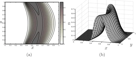
Figure 8. (a) A contour plot and (b) a surface plot of the cell volume fraction showing the
effect of a pressure-induced flow on tissue construct morphology att= 0.6. Parameter values:
h= 1,km= 4,kd= 0.1,D= 0.001, Pu= 1,Pd= 0.
0 0.1 0.2 0.3 0.4 0.5 0.6 0.7 0.8 0.9 1
0 0.1 0.2 0.3 0.4 0.5 0.6 0.7
n
[image:18.612.220.351.379.485.2]x t
Figure 9. The evolution of the centreline value of the cell volume fraction at successive times
t= 0−0.6 in steps oft≈0.05. Parameter values as in figure 8.
0 0.1 0.2 0.3 0.4 0.5 0.6 0.7 0.8 0.9 1 0 0.1 0.2 0.3 0.4 0.5 0.6 0.7 0.8 0.9 1 0 0.5 1 1.5 2 2.5 3 3.5 y x (a)
0 0.2 0.4 0.6 0.8 1 0
[image:19.612.147.431.89.210.2]0.5 1 0 1 2 3 4 5 p y x (b)
Figure 10. (a) A contour plot and (b) a surface plot showing the pressure distribution
corresponding to the tissue construct in figure 8. Parameter values as given in figure 8.
[image:19.612.217.355.263.366.2]0 0.2 0.4 0.6 0.8 1 0 0.5 1 0 0.2 0.4 0.6 0.8 1 1.2 u y x
Figure 11. A surface plot of the axial velocity profile corresponding to the tissue construct in
figure 8. Parameter values as given in figure 8.
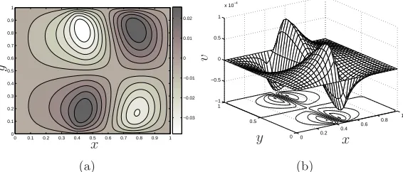
0 0.1 0.2 0.3 0.4 0.5 0.6 0.7 0.8 0.9 1
0 0.1 0.2 0.3 0.4 0.5 0.6 0.7 0.8 0.9 1 −0.03 −0.02 −0.01 0 0.01 0.02 y x (a) 0 0.2 0.4 0.6 0.8 1 0 0.5 1 −1 −0.5 0 0.5 1
x 10−4
v
y x
(b)
Figure 12. (a) A contour plot and (b) a surface plot showing the transverse velocity
corresponding to the tissue construct in figure 8. Parameter values as given in figure 8.
accounted for in a subsequent study. We remark that the solution for the axial velocity,u, is unique up to the addition of an arbitrary one-dimensional solution, ˆu; we have chosen ˆ
u= 0 so that no-slip is assured prior to the tissue; within and downstream from it the slip velocity is significant.
[image:19.612.146.429.424.545.2]Comparison of the profiles shown in figure 8 and the initial condition (4.1) shows that advection of the upstream periphery of the diffuse construct is greatest at the channel centreline (y=h/2) where the parabolic flow is maximal. Near the channel walls, where the flow speed is low, limited upstream movement is observed due to the presence of diffusion (for a larger diffusion coefficient than that employed in§3.2, this behaviour is, of course, also observed in the case of a one-dimensional diffuse tissue). Corresponding transverse variation is induced in the downstream periphery; however, it displays signif-icantly greater axial advection due to the greater flow speed there. In the absence of an imposed flow (Pu = 0 = Pd), the resulting cell population remains independent of the transverse coordinate. However, the population does not grow symmetrically about the midpoint of the initial distribution: the upstream periphery remains almost stationary while the downstream periphery spreads downstream (results omitted). In each case, this axially asymmetric advection behaviour is predicted by the one-dimensional, sharp interface analysis which indicates that the upstream interface moves at the speed of the imposed flow, the advection of the downstream interface being augmented by tissue growth (see equation (3.13)).
Figure 10 shows how the pressure distribution is affected by the presence of the cells. Up- and downstream from the tissue the pressure field decreases linearly with x; an increase in pressure is observed as the fluid flows through the area in which cells are present. As in the one-dimensional case (§3), the deviation from the linear pressure profile mirrors the cell distribution shown in figure 8. Similarly, the axial velocity profile shown in figure 11 is greatly affected by the cells’ presence. Upstream, the cells do not influence the flow anduremainsx-invariant; however, wheren6= 0 the axial flow speed increases with xin an approximately linear fashion, the gradient increasing with n as required by (2.18). Again, this behaviour was indicated by the one-dimensional analysis; see equations (3.9)–(3.11) and figure 5(b). We note that the choicesPu= 1,Pd= 0 set the velocity scale,U∗
w, used in the non-dimensionalisation (2.9) to be Uw∗ =Pu∗L∗/µ∗w. In the absence of cells, the maximum axial velocity is given byu∗=P∗
uh∗
2/(8µ∗
wL∗); for the parameter choice given we therefore expect the maximum upstream dimensionless velocity to beu= 1/8. Figure 11 confirms this.
The transverse component of velocity (v) is initially small due to the one-dimensional initial cell population. However, asnincreases, transverse variation is introduced within the tissue construct andvincreases, achieving maxima on the periphery of the construct (see figures 8 and 12). We note that the magnitude of the axial velocity,u, is much greater than the transverse velocity,v. This is because we impose an axial pressure gradient to drive the flow and, due to the no-penetration boundary conditions, the resistance to transverse motion in the channel is greater.
4.2 Mechanotransduction
illustrative purposes, we consider the response of the cells to the following stimuli: contact inhibition caused by cell-cell interactions, the effect of stress caused by increases in local cell density and the influence of the external fluid dynamics. The coupling is achieved by modifying the net mass production term,Sn. We remark that since the “cell” phase comprises cells and ECM, modifying the growth and death rates (km, kd) in response to local environmental factors enables crude modelling of a phenotypic switch due to mechanical stimuli from, for instance, a proliferative phase to an ECM-producing phase. The relevance of the following work hinges upon the appropriate choice of Sn. We restrict attention to the following cell density and pressure-dependent responses:
1. Cell density-dependent response: Sn = [km(n)−kd]n=κ(n)n; 2. pressure-dependent response: Sn = [km(p)−kd]n=κ(p)n,
in whichkm,kd are the rates of growth and death, respectively. For ease, the death rate kd is kept constant; the coupling of cell behaviour and the mechanical environment is captured entirely through the growth rate,km.
We now motivate these choices. Although not explicitly modelled, the choice km(n) enables us to capture the effect of contact inhibition [10] and tissue growth-induced stress [24, 57] on cell behaviour. Furthermore, since the pressure,p, represents a “lumped pressure” (p=pw0+n0Σn0; see§2.1), the choicekm(p) incorporates these considerations as well as the cells’ response to the culture medium pressure. The response of cells to culture medium pressure is well documented, especially with respect to bone tissue growth; for example, many authors have shown that bone cells respond to intermittent hydrostatic compression with diminished bone resorption and enhanced bone formation ([34] and references therein), increased adhesion [27] and increased osteopontin (a protein implicated in the bone remodelling process) expression [48]. Excessively high hydrostatic pressure (>200kPa) has been shown to exert an inhibitory effect on bone-specific gene expression [56].
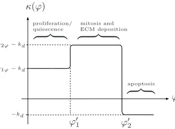
Considering first the density-dependent behaviour described above, we identify three distinct stages in the behaviour of the cell population: (i) a proliferative phase, (ii) an ECM-producing phase, and (iii) an apoptotic phase. At low density, the cells proliferate at a rate, km(n) = k1n; at intermediate density, due to the additional production of ECM, the growth rate of the cell phase is modified to a new value, km(n) = k2n (we assumek2n > k1n); finally, when the local density is too high, the cells enter an apoptotic phase (km(n) = 0) with death ratekd (we note that the “death rate”,kd includes ECM degradation as well as cell death). The threshold cell densities that separate these three types of behaviour are denotedn′
1 andn′2.
Similarly, in the pressure-dependent regime, we assume that at intermediate levels of pressure, the cells exhibit enhanced proliferation and ECM deposition (km(p) =k2p); at low pressure, the cells enter a quiescent state in which proliferation and ECM deposition is greatly reduced (km(p) =k1p< k2p); at excessively high levels, ECM deposition ceases and the cells become apoptotic (km(p) = 0). The corresponding thresholds are denoted p′
1,p′2.
for Sn; initial conditions are given by (4.1). We assume that the rates of growth and death of the cell phase (k1n,k1p,k2n,k2p,kd) are constant and represent the proliferative responses described above with a smoothed step function, as defined below:
κ(ϕ) =k2ϕ−k1ϕ
2 {tanh (g[ϕ−ϕ ′ 1])−1}
−k22ϕ{tanh (g[ϕ−ϕ′
2])−1} −kd. (4.2)
In (4.2),ϕrepresents the stimulus in question, with corresponding threshold valuesϕ′ 1,ϕ′2 and the parametergdictates the level of smoothing; we note that smoothing is necessary in order to obtain numerical solution. Figure 13 shows a sketch of the function k(ϕ), highlighting the progression from one phase to the next.
The effect of these choices of mass production term on the morphology of the resulting tissue is shown in figures 14 and 15.
ϕ κ(ϕ)
ϕ′
1 ϕ′2
k1ϕ−
kd
k2ϕ−kd
−kd
z }| { z }| {
z }| {apoptosis mitosis and
ECM deposition proliferation/
[image:22.612.201.378.251.382.2]quiescence
Figure 13. Schematic representation of the progression of a cell population through a number
of growth phases in response to a stimulus,ϕ=n, p.
0 0.1 0.2 0.3 0.4 0.5 0.6 0.7 0.8 0.9 1
0 0.1 0.2 0.3 0.4 0.5 0.6 0.7 0.8 0.9 1
0 0.1 0.2 0.3 0.4 0.5
y
x (a)
0 0.2
0.4 0.6
0.8
1 0
0.2 0.4
0.6 0.8
1
0 0.2 0.4 0.6 0.8
n
y x
(b)
Figure 14. (a) A contour plot and (b) a surface plot showing the effect of the cell
density-dependent proliferative response given by (4.2) on tissue construct morphology at t = 0.65. Parameter values: h= 1, k1n = 4, k2n = 5,kd= 0.1,n′1 = 0.5,n′2 = 0.6,g= 60,D = 0.001,
Pu= 1,Pd= 0.
Figure 14 illustrates that when the cells’ response is density-dependent, the growth of the cell phase is arrested atn=n′
[image:22.612.148.433.444.568.2]0 0.1 0.2 0.3 0.4 0.5 0.6 0.7 0.8 0.9 1 0
0.1 0.2 0.3 0.4 0.5 0.6 0.7 0.8 0.9 1
0 0.1 0.2 0.3 0.4 0.5
y
x (a)
0 0.2 0.4 0.6 0.8 1 0
0.5 1
0 0.1 0.2 0.3 0.4 0.5 0.6 0.7
n
y x
[image:23.612.146.431.89.210.2](b)
Figure 15. (a) A contour plot and (b) a surface plot showing the effect of the
pressure-dependent proliferative response given by (4.2) on tissue construct morphology at t = 0.8.
k1p= 5,k2p= 7,p′1= 0.5,p′2 = 0.8,g= 15; other parameter values as in figure 14.
and ECM-production (κ(n) =k2n−kd) to apoptosis (κ(n) =−kd). We note that despite the presence of apoptosis in this formulation, regression back to the proliferative phase ensures that the cell density does not fall belown=n′
2.
Figure 15 shows the response of the cell phase to pressure-dependent growth. Rather than being arrested at a threshold density the cells become apoptotic where the pressure is high (near the upstream diffuse interface and in regions of high cell density; see figure 10) and proliferation is reduced near x= 1 (where the pressure is low); between these regions, growth is enhanced. The result of this spatial variation in proliferative rate is a tissue construct which grows preferentially downstream in the regions of intermediate pressure.
Comparison of the cell phase distribution in each of the above growth regimes with that obtained in the case of constant growth and death rates (figures 8, 14 and 15) shows that the composition of the tissue construct is dramatically affected by coupling the growth response of the cells to their environment. When cell proliferation and ECM deposition are density-dependent, a uniform tissue construct is obtained; in the pressure-dependent case, the predicted tissue construct composition is far less uniform. It is interesting to note that in the absence of an imposed flow, the pressure field is directly proportional to the cell phase distribution (see equation (3.3)) and the cell density- and pressure-dependent responses are identical. Inspection of the morphology of tissue constructs produced in static and dynamic culture, together with the characteristic growth patterns predicted by this model, therefore provides a simple means to identify the dominant regulatory growth stimulus in a cell population.
5 Discussion
interphase drag, in which we may describe each phase as being subject to a common velocity and pressure field.
We have considered the effect of a dynamic flow environment on tissue growth pro-cesses. Analytic predictions were obtained in the limit of a one-dimensional growing tissue defined by two sharp interfaces, between which the cell density remains spatially invariant. The cell phase displayed logistic growth, the interfaces were advected by the ambient flow and the tissue width increased exponentially. The stability of this tissue to periodic transverse perturbations was investigated, and the interfaces were found to be unstable; the long-time stability being regulated only by the net growth rate. In the presence of a corresponding perturbation to the cell volume fraction, the perturbations to the upstream interface reversed sign due to the variation in construct density. This effect diminished with increasing perturbation wavenumber and decayed to zero for large time.
Using numerical simulations in one and two-dimensions, the behaviour of a diffuse tissue construct under an ambient flow was calculated for constant growth and death rates and the advection behaviour predicted by the sharp interface analysis was observed, indicating that this asymptotic limit captures much of the qualitative behaviour of the full system. In the two-dimensional model, transverse variation in the tissue construct density was induced by the parabolic flow of culture medium; small transverse flows were induced at the construct periphery.
Our analysis indicates that cells and ECM are advected through the bioreactor at the same speed as the imposed flow, implying that a long bioreactor and/or a low rate of perfusion is required in order to prevent the tissue from being flushed from the bioreactor before tissue growth can occur. This is a consequence of the simplifying limit of large interphase drag employed in this paper which demands that the cell and culture medium phases are subject to a common velocity field.
The proliferation/ECM deposition functions were chosen to reflect qualitatively a simple mechanotransduction mechanism. Our model admits more complex functional forms and dependence on combinations of the field variables; physiologically, it is ex-pected that these effects are integrated in a complex way to produce the cells’ overall response. The simple forms employed here allow clearer illustration of the importance of mechanotransduction-affected growth within a tissue growth modelling framework; how-ever, the mathematical formulation and numerical scheme developed is highly versatile, permitting the study of more complex functional forms and an investigation of the inter-play between many competing growth stimuli as appropriate experimental data become available.
The model employed here is applicable to tissue growth processes in which the solid characteristics of the system are unimportant. In a subsequent paper, we will present a three phase formulation in which we distinguish between the ECM and cell phases and consider mechanotransduction mechanisms in more detail. This more complex model will allow further predictions regarding the effect of perfusion the composition and mechanical integrity of the construct. Furthermore, the effect of cell-cell and cell-scaffold interactions on cell movement will be studied.
Acknowledgements
R.D.O is grateful for funding from the EPSRC and S.L.W acknowledges funding from the EPSRC in the form of an Advanced Research Fellowship. Collaboration with A. El-Haj (ISTM, Keele University) is also acknowledged. We thank the referees for their helpful comments.
References
[1] Araujo, R., McElwain, D.: A history of the study of solid tumour growth: The contribution of mathematical modelling. Bulletin of Mathematical Biology66(5), 1039–1091 (2004) [2] Araujo, R., McElwain, D.: A mixture theory for the genesis of residual stresses in growing
tissues I: A general formulation. SIAM Journal of Apllied Mathematics65(4), 1261–1284
(2005)
[3] Bhandari, R., Riccalton, L., Lewis, A., Fry, J., Hammond, A., Tendler, S., Shakesheff, K.: Liver Tissue Engineering: a Role for Co-culture Systems in Modifying Hepatocyte Function and Viability. Tissue Engineering7(3), 401–410 (2001)
[4] Bowen, R.: Theory of mixtures. Continuum Physics3, 1–127 (1976)
[5] Byrne, H., Chaplain, M.: Growth of nonnecrotic tumors in the presence and absence of inhibitors. Mathematical Biosciences130(2), 151–81 (1995)
[6] Byrne, H., King, J., McElwain, D., Preziosi, L.: A two-phase model of solid tumour growth. Applied Mathematics Letters16, 567–573 (2003)
[7] Byrne, H., Preziosi, L.: Modelling solid tumour growth using the theory of mixtures. Math-ematical Medicine and Biology20(4), 341 (2003)
[8] Cartmell, S., El Haj, A.: Bioreactors for tissue engineering, chap. 8. Springer (2005) [9] Chaplain, M.: Mathematical Modelling of Angiogenesis. Journal of Neuro-Oncology50(1),
37–51 (2000)
[11] Chaplain, M., McDougall, S., Anderson, A.: Mathematical modeling of tumor-induced an-giogenesis. Annual Review of Biomedical Engineering8(1), 233–257 (2006)
[12] Coletti, F., Macchietto, S., Elvassore, N.: Mathematical modeling of three-dimensional cell cultures in perfusion bioreactors. Industrial & Engineering Chemistry Research45(24),
8158–8169 (2006)
[13] Cowin, S.: How is a tissue built? Journal of Biomechanical Engineering122, 553 (2000)
[14] Cowin, S.: Tissue growth and remodeling. Annual Review of Biomedical Engineering6(1), 77–107 (2004)
[15] Curtis, A., Riehle, M.: Tissue engineering: the biophysical background. Physics in medicine and biology46, 47–65 (2001)
[16] Drew, D.: Averaged field equations for a two phase media. Studies in Applied Mathematics
L2, 205–231 (1971)
[17] Drew, D.: Mathematical modelling of two-phase flow. Annual Review of Fluid Mechanics
15, 261–291 (1983)
[18] Drew, D., Segel, L.: Averaged equations for two-phase flows. Studies in Applied Mathe-matics50, 205–231 (1971)
[19] El-Haj, A., Minter, S., Rawlinson, S., Suswillo, R., Lanyon, L.: Cellular responses to me-chanical loading in vitro. Journal of Bone and Mineral Research5(9), 923–32 (1990) [20] Forgacs, G., Foty, R., Shafrir, Y., Steinberg, M.: Viscoelastic Properties of Living Embryonic
Tissues: a Quantitative Study. Biophysical Journal74(5), 2227–2234 (1998)
[21] Franks, S.: Mathematical modelling of tumour growth and stability. Ph.D. thesis, University of Nottingham (2002)
[22] Franks, S., Byrne, H., King, J., Underwood, J., Lewis, C.: Modelling the early growth of ductal carcinoma in situ of the breast. Journal of Mathematical Biology 47, 424–452
(2003)
[23] Franks, S., King, J.: Interactions between a uniformly proliferating tumour and its sur-rounding: uniform material properties. Mathematical medicine and biology 20, 47–89 (2003)
[24] Fung, Y.: What are residual stresses doing in our blood vesels? Annals of Biomedical engineering19, 237–249 (1991)
[25] Greenspan, H.: Models for the growth of a solid tumor by diffusion. Stud. Appl. Math
51(4), 317–340 (1972)
[26] Hamilton, G., Westmoreland, C., George, E.: Effects of medium composition on the mor-phology and function of rat hepatocytes cultured as spheroids and monolayers. In Vitro Cellular and Developmental Biology - Animal37, 656–667 (2001)
[27] Haskin, C., Cameron, I., Athanasiou, K.: Physiological levels of hydrostatic pressure alter morphology and organization of cytoskeletal and adhesion proteins in MG-63 osteosar-coma cells. Biochemisty and Cell Biology71(1-2), 27–35 (1993)
[28] Higashiyama, S., Noda, M., Muraoka, S., Uyama, N., Kawada, N., Ide, T., Kawase, M., Kiyohito, Y.: Maintenance of hepatocyte functions in coculture with hepatic stellate cells. Biochemical Engineering Journal20, 113–118 (2004)
[29] Jaecques, S., Van-Oosterwyck, H., Muraru, L., Van-Cleynbreugel, T., De-Smet, E., Wevers, M., Naert, I., Vander-Sloten, J.: Individualised, microCT-based finite element modelling as a tool for biomechanical analysis relating to tissue engineering of bone. Biomaterials
25, 1683–1696 (2004)
[30] Karp, J., Sarraf, F., Shoichet, M., Davies, J.: Fibrin-filled scaffolds for bone-tisue engineer-ing. Journal of Biomedical Materials Research71A, 162–171 (2004)
[31] Keller, E., Segel, L.: Initiation of slime-mold aggregation viewed as an instability. Journal of Theoretical Biology26(3), 399–415 (1970)
[32] Keller, E., Segel, L.: Model for chemotaxis. Journal of Theoretical Biology30(2), 225–234 (1971)
[34] Klein-Nulend, J., Roelofsen, J., Sterck, J., Semeins, C., Burger, E.: Mechanical loading stimulates the release of transforming growth factor-beta activity by cultured mouse calvariae and periosteal cells. Journal of Cell Physiology 163(1), 115–119 (1995) [35] Kolev, N.: Multiphase Flow Dynamics, vol. 1 - Fundamentals. Springer (2002)
[36] Lemon, G., King, J.: Multiphase modelling of cell behaviour on artificial scaffolds: effects of nutrient depletion and spatially nonuniform porosity. Mathematical Medicine and Biology24(1), 57 (2007)
[37] Lemon, G., King, J., Byrne, H., Jensen, O., Shakesheff, K.: Multiphase modelling of tissue growth using the theory of mixtures. Journal of Mathematical Biology 52(2), 571–594 (2006)
[38] Lewis, M., Macarthur, B., Malda, J., Pettet, G., Please, C.: Heterogeneous proliferation within engineered cartilaginous tissue: the role of oxygen tension. Biotechnology and Bioengineering91(5), 607–15 (2005)
[39] Lubkin, S., Jackson, T.: Multiphase Mechanics of Capsule Formation in Tumors. Journal of Biomechanical Engineering124, 237 (2002)
[40] Luca, M., Chavez-Ross, A., Edelstein-Keshet, L., Mogilner, A.: Chemotactic signalling, mi-croglia, and alzheimer’s disease senile plaques: is there a connection? Bulletin of Mathe-matical Biology65, 696–730 (2003)
[41] Ma, M., J.S., X., Purcell, W.: Biochemical and functional changes of rat liver spheroids during spheroid formation and maintenance in culture. Journal of Cellular Biochemistry
90, 1166–1175 (2003)
[42] Maggelakis, S.: Mathematical model of prevascular growth of a spherical carcinoma. Math-ematical and Computer Modelling13(5), 23–38 (1990)
[43] Malda, J., Rouwkema, J., Martens, D., le Comte, E., Kooy, F., Tramper, J., van Blitterswijk, C., Riesle, J.: Oxygen gradients in tissue-engineered Pegt/Pbt cartilaginous constructs: Measurement and modeling. Biotechnology and Bioengineering86(1), 9–18 (2004) [44] Marle, C.: On macroscopic equations governing multiphase flow with diffusion and chemical
reactions in porous media. International Journal of Engineering Science20(5), 643–662 (1982)
[45] Martin, I., Wendt, D., Heberer, M.: The role of bioreactors in tissue engineering. Trends in Biotechnology22(2), 80–86 (2004)
[46] McGarry, J., Klein-Nulend, J., Mullender, M., Prendergast, P.: A comparison of srain and fluid shear stress in simulating bone cell responses - a computation and experimental study. The FASEB Journal18(15) (2004)
[47] Murray, J.: Mathematical Biology. Springer (2002)
[48] Owan, I., Burr, D., Turner, C., Qiu, J., Tu, Y., Onyia, J., Duncan, R.: Mechanotransduction in bone: osteoblasts are more responsive to fluid forces than mechanical strain. American Journal of Physiology- Cell Physiology 273(3), 810–815 (1997)
[49] Palsson, E.: A three-dimensional model of cell movement in multicellular systems. Future Generation Computer Systems17, 835–852 (2001)
[50] Palsson, E., Othmer, H.G.: A model for individual and collective cell movement in Dic-tyostelium discoideum. PNAS97(19), 10,448–10,453 (2000)
[51] Porter, B., Zauel, R., Stockman, H., Guldberg, R., Fyhrie, D.: 3-D computational modeling of media flow through scaffolds in a perfusion bioreactor. Journal of Biomechanics38(3), 543–549 (2005)
[52] Powers, M., Griffith, L.: Adhesion-guided in vitro morphogenesis in pure and mixed cell cultures. Microspcopy research and technique43, 379–384 (1998)
[53] Powers, M., R.E., R., Griffith, L.: Cell-substratum adhesion strength as a determinant of hepatocyte aggregate morphology. Biotechnology and bioengineering20(4), 15–26 (1997)
[54] Raimondi, M.: The effect of media perfusion on three-dimensional cultures of human chon-drocytes: Integration of experimental and computational approaches. Biorheology41(3), 401–410 (2004)
of Functional Liver Tissue: Three-Dimensional Coculture of Primary Hepatocytes and Stellate Cells. Tissue Engineering9(3), 401–410 (2003)
[56] Roelofsen, J., Klein-Nulend, J., Burger, E.: Mechanical stimulation by intermittent hydro-static compression promotes bone-specific gene expression in vitro. Journal of Biome-chanics28(12), 1493–1503 (1995)
[57] Roose, T., Neti, P., Munn, L., Boucher, Y., Jain, R.: Solid stress generated by spheroid growth estimated using a poroelasticity model. Microvascular Research 66, 204–212
(2003)
[58] Salgado, A., Coutinho, O., Reis, R.: Bone tissue engineering: State of the art and future trends. Macromolecular Bioscience 4, 743–765 (2004)
[59] Sherratt, J., Dallon, J.: Theoretical models of wound healing: past successes and future challenges. Comptes Rendus Biologies325(5), 557–64 (2002)
[60] Sipe, J.: Tissue Engineering and Reparative Medicine. Annals of the New York acadamy of Sciences961, 1–9 (2002)
[61] Sutherland, R., Sordat, B., Bamat, J., Gabbert, H., Bourrat, B., Mueller-Klieser, W.: Oxy-genation and differentiation in multicellular spheroids of human colon carcinoma. Cancer Research46(10), 5320–5329 (1986)
[62] Tracqui, P., Ohayon, J.: Transmission of mechanical stresses within the cytoskeleton of adgerent cells: a theoretical analysis based on a multi-component cell model. Acta Bio-theoretica52, 323–341 (2004)
[63] Whitaker, S.: The transport equations for multi-phase systems. Chemical Engineering Science28, 139–147 (2000)
[64] Wood, M., Marshall, G., Yang, Y., El Haj, A.: Seeding efficiency and distribution of primary osteoblasts in 3D porous poly (L-lactide) scaffolds. European Cells and Materials6, 58 (2003)