The algorithm of Bayesian estimation of maternal genetic and permanent maternal environmental variances in a two trait binary threshold model

In recent years significant reconstructions have

been done in the programs of genetic improvement

of farm animals. Although long-term selection for

the improvement of production traits has reached

the assumed objectives, it has also contributed to

the degradation of the so-called functional traits

(Hansen, 2000). Most production traits are

geneti-cally and phenotypigeneti-cally continuous. For this

rea-son linear models could be successfully used for

their analysis. However, even though determined

by the number of loci, some functional traits are

discontinuous variables. They are called threshold

traits. Many of them, for instance fertility,

hatch-ability or resistance to certain diseases are binary

traits.

In order to take into consideration the specific

character of threshold traits, threshold models are

used for their analysis (Gianola and Foulley, 1983;

Harville and Mee, 1984). In these models it is

as-sumed that the phenotypic categorized variability

of a trait is determined by the values of a certain

unobserved random continuous variable, called

li-ability. This variable is linked with the limits of

cat-egories (thresholds), i.e. the observation is classified

on the basis of the phenotype to a given category

if the value of the unobserved variable exceeds the

threshold of this category (also unobserved). In

the hidden scale standard deviation of the

unob-served variable is used as the unit of measurement

(Falconer, 1989). In the case of two categories it is

assumed, without the loss of generality, that the

threshold between these categories lies at point 0

(Gianola and Foulley, 1983; Misztal

et al.

, 1989).

Threshold models are an effective alternative to

data transformation. It was shown that the adoption

of such models gives more accurate estimates of

genetic parameters (Matos

et al.

, 1997; Abdel-Azim

and Berger, 1999; Dobek

et al.

, 2003).

Some of the threshold traits have a complex

genet-ic background. They may be determined to a large

extent by indirect maternal effects, both genetic and

environmental ones (Sewalem, 1989). In this paper

we extend a previously described model (Moliński

et al.

, 2003) by the genetic maternal and permanent

environmental effects. We present an algorithm for

the estimation of genetic parameters in a two-trait

The study was conducted within the research project of the Commi�ee for Scientific Research (Grant No. 5 P06 D 02019).

The algorithm of Bayesian estimation of maternal

genetic and permanent maternal environmental

variances in a two-trait binary threshold model

E. S���������

1

, M. S���������

2

, A. D����

1

, K. M�������

1

, T. S�����������

2

1

Department of Mathematical and Statistical Methods,

2

Department of Genetics and Animal

Breeding, August Cieszkowski Agricultural University of Poznań, Poland

ABSTRACT: The paper presents an algorithm for the estimation and prediction of parameters in a two-trait binary threshold model. The model includes fixed effects and the following random effects: genetic direct additive, genetic maternal additive and permanent maternal environmental effects. The Gibbs sampling procedure was used to estimate the parameters. The algorithm was illustrated with a numerical example showing appropriateness of the proposed method.

model when the interesting traits are threshold

traits with two categories (binary traits).

MODEL

Let us consider the vector of observations

y

. The

components of

y

are taking values 0 or 1. The value

of

y

is conditioned by an unobservable vector

w

(liabilities). When

w

is positive, the phenotypic

expression

y

is 1, otherwise it is 0. For the vector

w

we are assuming the following model:

where:

and

w(k) _{= the N-vector of the values of the unobserved}

random variable(liability) β(k) _{= the p-vector of fixed effects}

a(k) _{= the q-vector of random genetic direct additive}

effects

m(k) _{= the q-vector of random genetic maternal}

tive effects

c(k) _{= the v-vector of random permanent maternal}

environmental effects

e(k) _{= the N-vector of effects of residuals for the k-th}

trait, k = 1, 2

I = the identity matrix of a given dimension X, Z₁, Z₂, Z₃ = known matrices of corresponding dimensions with elements equal to 0 or 1

Further:

n = the number of observed animals

, while n_i is the number of observations (equal for two traits) for the i-th animal

q = the number of all the investigated animals

v = the number of dams

For the model parameters the following

assump-tions are adopted:

Moreover:

where: A = the q x q additive relationship matrix (Quaas, 1976)

σ2

ak = the genetic direct additive variance for

k-th trait σ2

mk = the genetic maternal additive variance

for k-th trait σ_a

kak’ = the covariance between direct additive

effects for k-th and k’-th traits σ_a

kmk’ = the covariance between direct and maternal

additive effects for k-th and k’-th traits σ_m

kmk’ = the covariance between maternal additive

effects for k-th and k’-th traits σ2

ck = the permanent maternal environmental

variance

k = 1, 2, k’ = 1, 2

ESTIMATION OF PARAMETERS

Estimators and predictors of unknown model

parameters may be obtained by Gibbs sampling

(Sørensen

et al.

, 1995; Moliński

et al.

, 2003). In the

Gibbs sampling method, the values of the

param-eter are generated from its

a posteriori

conditional

distribution, assuming all the other parameters are

known. The generated values may be treated as a

sample from corresponding marginal distribution,

when the condition of the stationarity of the process

is satisfied. Let us adopt the following assumptions

concerning the conditional distributions for the

pa-rameters (Sørensen

et al.

, 1995):

w_lj(k)_{| all the other parameters and y}

lj(k) = 1 ~ N(x_ljβ(k) _{+ z}

1_lja(k) + z2_ljm(k) + z3_ljc(k) ; 1) (le�-truncated)

w_lj(k)_{| all the other parameters andy}

lj(k) = 0 ~ N(x_ljβ(k) _{+ z}

1_lja(k) + z2_ljm(k) + z3_ljc(k) ; 1) (right-truncated) where: y_lj(k) _{= the j-th observation of the k-th trait for the}

l-th animal (y_lj(k)_{= 1or y} lj(k)= 0)

x_lj, z_1lj, z_2lj, z_3lj = the lj-th row of corresponding

matrices

l = 1, 2, ..., n j = 1, 2, ..., n_l

Let the inverses of

V

_u

and

V

_c

be:

Elements of vectors

β, a, m, c

are generated from

normal distributions, the parameters of which are

determined from the formulas given below:

� � � � � � � � � ₍(₂1)₎

w w w , � � � � � � � � � � � � � � � � � � � � � � � � � � � � � � � � � � � � � � � � � � � �

� (₍1₂₎) , ₍(1₂)₎, (₍1₂)₎ , ₍(1₂)₎ , (₍₂1)₎ e e e c c c m m m a a a � � � � � �n

i ni N 1 e c Z I m Z I a Z I � X I

w�( 2� ) �( 2� 1) �( 2� 2) �(2� 3) �

) , ( ~ 2 ) ( k a q k _{N 0A�}

a , m(k)~Nq(0,A�2m_k), ()~ v( , v 2ck) k _{N 0I�}

c , e(k)~NN(0,IN)

A V A m a m a

u � � u�

� � � � � � � � � � � � � � � � � � � � � � � � � � � � � � � � � � 2 2 2 1 1 2 ) 2 ( ) 2 ( ) 1 ( ) 1 ( 2 2 2 2 1 2 1 2 2 2 1 2 2 1 2 1 1 2 1 1 2 1 2 1 1 1 ) ( m m a m m m a m a a m a a a m m m a m m a m a a a m a a � � � � � � � � � � � � � � � � Var Var v v c c � � Var

Var I V I

c c

c � � _c�

� � � � � � � � � � � � � � � � � � ₂ 2 ) 2 ( ) 1 ( 2 1 0 0 ) ( 0 c m 0 c

a; )� , ( ; )�

( Cov Cov � � � � � � � � � � � � � � 44 34 24 14 34 33 23 13 24 23 22 12 14 13 12 11 1 d d d d d d d d d d d d d d d d u

V

,

_�

i) fixed effects (

i

= 1, ...,

p

;

k

= 1, 2):

ii) genetic direct additive effects (

i

= 1, ...,

q

):

iii) genetic maternal additive effects (

i

= 1, ...,

q

):

iv) permanent maternal environmental effects (

i

=

1, ...,

v

):

where: Aii _{= the i-th diagonal element of A}–1

Ai. _{= the i-th row vector of A}–1

Ai, –i _{= the i-th row vector of A}–1 _{with the i-th}

ment skipped a(k)

–i , m(–ki )= vectors a(k) and m(k) with i-th element removed

x_i, z_1i, z_2i, z_3i = the i-th columns of corresponding matrices

The distributions for unknown components of

variance and covariance are as follows:

V_u| all the other parameters~IW₄[(U1A–1_U)–1_{, q]}

where: U = [a(1)_{, m}(1)_{, a}(2)_{, m}(2)_]

σ2

ck| all the other parameters~

and IW denotes inverted Wishart distribution

SIMULATION STUDY

Data

The correctness of the proposed algorithm was

checked through simulation studies. Therefore we

simulated a female-limited trait for a real pedigree.

The pedigree was taken from a layer flock and

con-sisted of 9 generations, 6 476 birds, including 5 980

with known parents, out of which 5 353 were female.

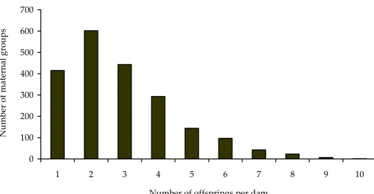
The distribution of the size of maternal groups is

given in Figure 1. For each dam two binary traits

were generated in 30 replications (corresponding to

the average number of eggs destined for hatching).

The simulation

of data was conducted in two stages.

] ) (' [ ) ' ( ) ( ) 2 ( . 14 ) 2 ( . 13 ) 1 ( . 12 ) 1 ( , 11 ) 1 ( 3 ) 1 ( 2 ) 1 ( ) 1 ( 1 1 11 1 1 ) 1 ( m A a A m A a A c Z m Z X� w z A z z a i i i i i i i ii i i i d d d d d E � � � � � � � � � � � � 1 11 1 1 ) 1 ( _{) ( ' )}

( _i � _{i i}�d ii �

Vara z z A

] ) (' [ ) ' ( ) ( ) 1 ( . 23 ) 1 ( . 13 ) 2 ( . 34 ) 2 ( , 33 ) 2 ( 3 ) 2 ( 2 ) 2 ( ) 2 ( 1 1 33 1 1 ) 2 ( m A a A m A a A c Z m Z X� w z A z z a i i i i i i i ii i i i d d d d d E � � � � � � � � � � � � 1 33 1 1 ) 2 ( _{) ( ' )}

( _{� �} ii �

i i

i d

Vara z z A

] ) (� [ ) � ( ) ( ) 2 ( . 24 ) 2 ( . 23 ) 1 ( , 22 ) 1 ( . 12 ) 1 ( 3 ) 1 ( 1 ) 1 ( ) 1 ( 2 1 22 2 2 ) 1 ( m A a A m A a A c Z a Z X� w z A z z m i i i i i i i ii i i i d d d d d E � � � � � � � � � � � � 1 22 2 2 ) 1 ( _{) ( � )}

( _i � _{i i}�d ii �

Varm z z A

] ) (� [ ) � ( ) ( ) 1 ( . 24 ) 1 ( . 14 ) 2 ( , 44 ) 2 ( . 34 ) 2 ( 3 ) 2 ( 1 ) 2 ( ) 2 ( 2 1 44 2 2 ) 2 ( m A a A m A a A c Z a Z X� w z A z z m i i i i i i i ii i i i d d d d d E � � � � � � � � � � � � 1 44 2 2 ) 2 ( _{) ( � )}

( _i � _{i i}�d ii �

Varm z z A

) (' ) ' ( )

( (ik) i i 1 i (k) 1 (k) 2 (k) 3 (k)

E� � x x � x w �Za �Z m �Zc

1 )

( _{) ( ' )} ( ik � i i �

Var� x x

)] (' [ ) ' ( )

(c(i1) � z3iz3i�d55 �1z3i w(1)�X�(1)�Z1a(1)�Z2m(1) E 1 55 3 3 ) 1 ( _{) ( ' )}

( � �d �

Varci z izi

)] (' [ ) ' ( )

(ci(2) � z3iz3i�d66�1z3i w(2)�X�(2)�Z1a(2)�Z2m(2) E 1 66 3 3 ) 2 ( _{) ( ' )}

( � �d �

Varci z iz i

2 ) ( )' ( ₎ ( v k k � c c 0 100 200 300 400 500 600 700

1 2 3 4 5 6 7 8 9 10

Number of offsprings per dam

[image:3.595.115.482.542.732.2]

N um be r o f m at er na l g ro up s

In the first stage, elements of vector

w

were

gener-ated according to the studied model with one fixed

effect. The assumed true values of the components

of variance and covariance as well as the levels of

fixed effect are presented in Table 1. In the second

stage variables

y

_lj

were determined based on the

pre-viously obtained vector

w

. The true values of the

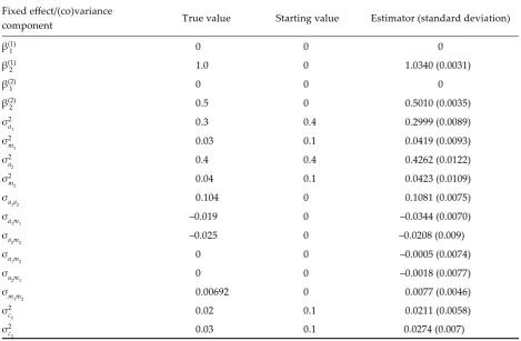
parameters used in simulation are given in Table 1.

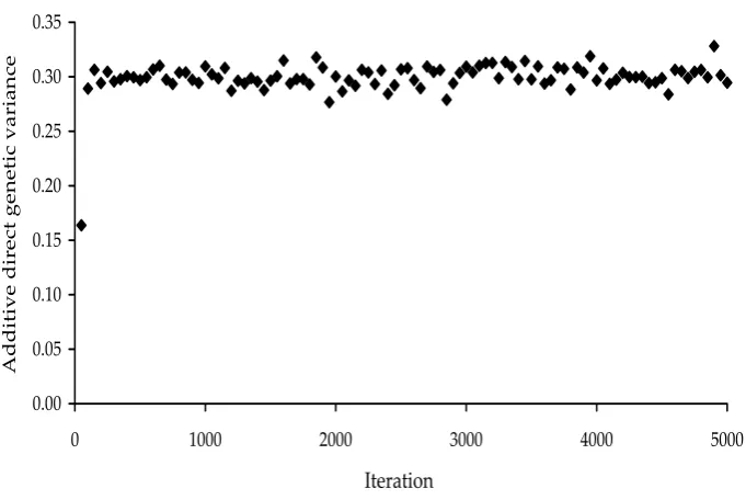
Results

The stationarity of the process is illustrated by

random values for direct additive genetic variance

σ

2

a₁

(Figure 2). Similar stationarity of the random

process was observed for other parameters as well.

Point estimators and predictors of parameters of the

model were calculated as averages from 20 000

ran-dom values coming from each 50-th iterative step.

The starting values and estimates of parameters are

presented in Table 1. The obtained results indicate

the correctness of the method, the estimators of

parameters are close to the true values.

PRACTICAL IMPLICATIONS

As it was already mentioned, the proposed

algo-rithm exhibits good properties especially

concern-ing the low values of the estimated parameters.

Roughsedge

et al

. (2001) reported that the

accu-racy of the estimation of maternal variances was

positively correlated with the actual value of this

parameter.

[image:4.595.62.532.103.410.2]

It needs to be mentioned that the satisfactory

re-sults were obtained for the population whose size

Table 1. The results of simulation studies – estimators of fixed effects and variance and covariance components

Fixed effect/(co)variance

component True value Starting value Estimator (standard deviation) β(1)

1 0 0 0

β(1)

2 1.0 0 1.0340 (0.0031)

β(2)

1 0 0 0

β(2)

2 0.5 0 0.5010 (0.0035)

σ2

a₁ 0.3 0.4 0.2999 (0.0089)

σ2

m1 0.03 0.1 0.0419 (0.0093)

σ2

a₂ 0.4 0.4 0.4262 (0.0122)

σ2

m2 0.04 0.1 0.0423 (0.0109)

σ_a

1a2 0.104 0 0.1081 (0.0075)

σ_a

1m1 –0.019 0 –0.0344 (0.0070)

σ_a

2m2 –0.025 0 –0.0208 (0.009)

σ_a

1m2 0 0 –0.0005 (0.0074)

σ_a

2m1 0 0 –0.0018 (0.0077)

σ_m

1m2 0.00692 0 0.0077 (0.0046)

σ2

c1 0.02 0.1 0.0211 (0.0058)

σ2

c2 0.03 0.1 0.0274 (0.007)

Note on symbols: β(k)

1 = the first level of the fixed effect for k-th trait, β(k2) = the second level of the fixed effect for k-th trait, σ2ak = the genetic

direct additive variance for k-th trait, σ2

mk = the genetic maternal additive variance for k-th trait, σakak’ = the covariance

between direct additive effects for k-th and k’-th traits, σ_a

kmk’ = the covariance between direct and maternal additive

effects for k-th and k’-th traits, σ_m

kmk’ = the covariance between maternal additive effects for k-th and k’-th traits, σ 2

ck =

and structure were not very suitable for the

esti-mation of maternal genetic environmental effects

(Figure 1). It indicates considerable universality of

the proposed method. On the other hand, further

simulation studies are required. They should

con-sider pedigrees of different size and structure.

REFERENCES

Abdel-Azim G.A., Berger P.J. (1999): Properties of thresh-old model predictions. J. Anim. Sci., 77, 582–590. Dobek A., Szydłowski M., Szwaczkowski T., Skotarczak

E., Moliński K. (2003): Bayesian estimates of genetic variance of fertility and hatchability under a threshold animal model. J. Anim. Feed Sci., 12, 307–314. Falconer D.S. (1989): Introduction to Quantitative

Genet-ics. Third edition. Longman Scientific and Technical. John Wiley and Sons, Inc., New York.

Gianola D., Foulley J.L. (1983): Sire evaluation for ordered categorical data with a threshold model. Génét. Sél. Evol., 15, 201–224.

Hansen L.B. (2000): Consequences of selection for milk yield from a geneticist’s viewpoint. J. Dairy Sci., 83, 1145–1150.

Harville D.A., Mee R.W. (1984): A mixed – model proce-dure for analysing ordered categorical data. Biometrics,

40, 393–408.

Matos C.A.P., Thomas D.L., Gianola D., Perez-Enciso M., Young L.D. (1997): Genetic analysis of discrete repro-ductive traits in sheep using linear and nonlinear models. I. Estimation of genetic parameters. J. Anim. Sci., 75, 76–87.

Misztal I., Gianola D., Foulley J.L. (1989): Computing aspects of a nonlinear method of sire evaluation for categorical data. J. Dairy Sci., 72, 1557–1568.

Moliński K., Szydłowski M., Szwaczkowski T., Dobek A., Skotarczak E. (2003): An algorithm for genetic variance estimation of reproductive traits under a threshold model. Arch. Tierzucht, 46, 85–91.

Quaas R.L. (1976): Computing the diagonal elements and inverse of a large numerator relationship matrix. Bio-metrics, 32, 949–953.

Roughsedge T., Brotherstone S., Visscher P.M. (2001): Bias and power in the estimation of a maternal family variance components in the presence of incomplete and incorrect pedigree information. J. Dairy Sci., 84, 944–950.

Sewalem A. (1998): Genetic study of reproduction traits and their relationship to production traits in White Leghorn lines. [PhD thesis.] Swedish University of Agricultural Sciences, Uppsala.

Sørensen D.A., Andersen S., Gianola D., Korsgaard I. (1995): Bayesian inference in threshold model using Gibbs sampling. Genet. Sel. Evol., 27, 229–249.

[image:5.595.124.465.81.309.2]

Received: 03–07–14 Accepted a�er corrections: 03–12–29 Figure 2. The Gibbs sampling process – the first 5 000 samples for the direct additive genetic variance

2

0.00

0.05 0.10 0.15 0.20 0.25 0.30 0.35

0 1000 2000 3000 4000 5000

Iteration

A

d

d

it

iv

e

d

ir

ec

t

g

en

et

ic

v

ar

ia

n

ABSTRAKT

Algoritmus Bayesovského odhadu maternálně genetických a permanentních maternálně genetických

variancí ve dvouznakovém binárním prahovém modelu

V práci je předložen algoritmus pro odhad a předpověď parametrů ve dvouznakovém binárním prahovém modelu. Tento model obsahuje pevné efekty a následující náhodné efekty: genetické přímé aditivní, genetické mateřské adi-tivní a efekty trvalého mateřského prostředí. Pro odhad parametrů byl použit postup Gibbsova výběru. Algoritmus byl znázorněn na numerickém příkladě, který prokázal vhodnost navržené metody.

Klíčová slova: binární znaky; genetické efekty; Gibbsův výběr; prahový model; maternální efekty

Corresponding Author

Prof. Dr. Tomasz Szwaczkowski, Department of Genetics and Animal Breeding, August Cieszkowski Agricultural University, Wołyńska 33, PL 60-637 Poznań, Poland