Optimal Experimental Design for Predator-Prey
Functional Response Experiments
Jeff F. Zhang†, Nikos E. Papanikolaou∗,∗∗,∓, Theodore Kypraios] and Christopher C. Drovandi†,‡
† School of Mathematical Sciences, Queensland University of Technology, Australia
‡ Australian Centre of Excellence for Mathematical and Statistical Frontiers (ACEMS) ∗Directorate of Plant Protection,
Greek Ministry of Rural Development and Food, Athens, Greece
∗∗ Laboratory of Agricultural Zoology and Entomology, Agricultural University of Athens, Greece.
∓ Benaki Phytopathological Institute, Athens, Greece
]School of Mathematical Sciences, University of Nottingham, United Kingdom
email: [email protected]
July 22, 2018
Abstract
Functional response models are important in understanding predator-prey in-teractions. The development of functional response methodology has progressed from mechanistic models to more statistically motivated models that can ac-count for variance and the over-dispersion commonly seen in the datasets col-lected from functional response experiments. However, little information seems to be available for those wishing to prepare optimal parameter estimation designs for functional response experiments. It is worth noting that optimally designed experiments may require smaller sample sizes to achieve the same statistical outcomes as non-optimally designed experiments. In this paper, we develop a model-based approach to optimal experimental design for functional response experiments in the presence of parameter uncertainty (also known as a robust optimal design approach). Further, we develop and compare new utility func-tions which better focus on the statistical efficiency of the designs; these utilities are generally applicable for robust optimal design in other applications (not just in functional response). The methods are illustrated using a beta-binomial functional response model for two published datasets: an experiment involving
the freshwater predatorNotonecta glauca (an aquatic insect) preying onAsellus
aquaticus(a small crustacean), and another experiment involving a ladybird
fabae Scopoli). As a by-product, we also derive necessary quantities to perform optimal design for beta-binomial regression models, which may be useful in other applications.
Keywords: D-optimality, exchange algorithm, Fisher information, functional response,
1
Introduction
Models of predator-prey interactions where the rate of predation varies according to the availability of prey are termed functional response models. Typical models deal with single predator, multiple prey scenarios (usually over a finite area), and the aim is to predict the number of prey attacked or consumed as a function of the number of prey available (prey density). Such models are important as they form “one of the cornerstones of prey-predator interactions” (Casas and Hulliger, 1994), which in turn underpins almost all ecological systems.
The study of functional responses is an active area of research, determining the dynamics and stability of predator-prey systems (Oaten and Murdoch, 1975). Moreover, ecologists often utilise functional response models in order to test several hypotheses. A selection
of recent examples include: a study of the predatory behaviour of wolves (Canis lupus)
against a managed population of moose (Aleces alces) in Scandinavia (Zimmermann et al.,
2015); an examination of the impact of predator and prey size on the functional response in mosquito-predator systems (Weterings et al., 2015); a study to better understand predator-prey systems in the ocean via computer simulation of functional response (Accolla et al., 2015); a study of how the spatial arrangement of prey affects the functional response (Hossie and Murray, 2016); and an investigation on the effect of mutual interference on the predation behavior of ladybird beetles (Papanikolaou et al., 2016b). In addition, the importance of functional response in invasion ecology has been recently highlighted (Dick et al., 2017). Given these points, an accurate estimation of functional response parameters and outcome is highly desirable for ecologists.
In functional response experiments, the number of prey N used for each observation in
the experiment is often controlled. This is biologically feasible as ecologists are usually approximately aware of the predation ability of the selected terrestrial or aquatic species, based on observations on their laboratory cultures and/or preliminary experiments. Fenlon and Faddy (2006) give an excellent account of the development of statistical models to account for the variability of data collected from functional response experiments. Some of the seminal work in this area include Trexler et al. (1988) and Casas and Hulliger (1994). Fenlon and Faddy (2006) themselves compare several models with a variety of equations modelling the mean, and use either binomial or beta-binomial modelling of the variance
for each value ofN.
However, despite the development of more statistically-driven models and the substantial amount of research activity in the general area of functional response experiments hith-erto, there has been little attention given to optimally designing such experiments for the purpose of efficient parameter estimation. To the best of our knowledge, there are no pub-lished functional response experiments that express any statistical methodology behind the design points chosen. Our contribution is significant since functional response experi-ments can by their nature be expensive and/or difficult to conduct (Stenseth et al., 2004); optimally designed experiments are advantageous in that they allow model parameters to be estimated with maximum efficiency and precision, potentially reducing the number of experimental runs necessary. In this paper, we develop an optimal design method for the efficient estimation of model parameters in functional response experiments, using a case study based on an experiment conducted by Hassell et al. (1977). The same methods are applied to an additional dataset from Papanikolaou et al. (2016a) to demonstrate the efficacy of our approach.
the model. Such designs are referred to as locally optimal designs. However, there is often uncertainty in the parameter values of the model being designed for, and it is important for experimental designs to be robust, i.e. to perform reasonably well under a variety of parameter configurations that might be plausible. Such designs are referred to as robust designs in the literature (Walter and Pronzato, 1987; Woods et al., 2006; Gotwalt et al., 2009). The uncertainty in the model parameter can be characterised with a probability, or ‘prior’, distribution, from which a finite sample of parameter values can be drawn. A common approach to obtaining robust designs is the pseudo-Bayesian method (Walter and Pronzato, 1987), where the utility to be optimised is an average over the utilities for different parameter values. The maximin approach (e.g. Dette (1997)) maximises the lowest utility over the parameter set.
In this paper we also develop some new utilities for robust designs. These novel utilities consider i) the variability in the utility values and ii) maximising the efficiency (utility value divided by the utility of the locally optimal design for some parameter configuration) rather than the raw utility values, to help mitigate scaling problems for different parameter configurations.
A markedly different approach to obtaining robust designs is suggested by Dror and Stein-berg (2006). They first calculate locally optimal designs for each parameter value, and then perform a clustering analysis to obtain a robust design, without needing to optimise over a robust utility. These methods are computationally more efficient, but their cluster-ing analysis is only applicable to continuous design spaces. In this paper, we also develop an analogous approach for integer-valued designs, which is straightforward to implement and provides an additional robust design (generated using a non-utility based method) to compare with.
The case study that we consider involves a beta-binomial regression model, so we derive the necessary quantities required to perform optimal design for such models, which may be useful in other applications.
The paper is outlined as follows. Section 2.1 describes a motivating case study. Utility functions often used for parameter estimation are detailed in Section 2.2, which includes some new approaches to robust design. The method we use to efficiently maximise a chosen utility function is described in Section 2.3. The results for the two case studies are presented in Section 3. Finally, Section 4 concludes with a discussion.
2
Materials and Methods
2.1 Case Study
To demonstrate the methods highlighted in this paper, we consider re-designing two pub-lished functional response experiments. In this section, we first give some background to functional response and define the design problem. To illustrate the ideas and concepts laid out in this section, we use the first case study (Case Study I) as a running example. In Section 3 we present results for Case Study I and Case Study II.
0 20 40 60 80 100 Number of prey available (N) 0
10 20 30
[image:5.595.176.409.96.286.2]Number predated (n)
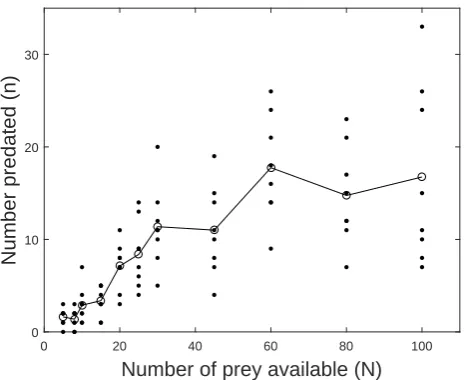
Figure 1: Original data from Hassell et al. (1977): individual sample values (·), sample
means (◦−◦−◦) for each value of N. See Trexler et al. (1988) and Casas and Hulliger
(1994) for the raw data values.
n= rN T
1 +rThN
, (1)
where n is the number of prey consumed/attacked, N is the available number of prey
(in a given area), T is the total duration of the experiment, which is always fixed and
predefined such that the interpretation of the model estimated parameters is consistent
across the experiment, Th is the handling time per prey attacked and r reflects the per
capita prey consumption in low prey densities, which determines the initial slope of the functional response curve. When prey is depleted during the experiment, the differential form of the disc equation (see, for example, Papanikolaou et al. (2016a) for more details)
is to be used. The parameters of interest areTh and r.
In order to learn about a particular predator-prey interaction, experiments are conducted where varying numbers of prey (the design variable) are made available to a predator, with the number of prey attacked or consumed in a finite period of time recorded as the
response variable. We assume thatK observations of the predator-prey system are to be
obtained and we denote the number of prey to use for observationiasNi and the vector
of prey numbers for all observations asN = (N1, . . . , NK). The corresponding observed
number of predated prey for the ith observation is denoted ni and the full dataset as
n = (n1, . . . , nK). An example dataset from a typical functional response experiment
is shown in Figure 1. The original data was collected by Hassell et al. (1977) from an
experiment involving the freshwater predatorNotonecta glauca (an aquatic insect) preying
onAsellus aquaticus (a small crustacean resembling a woodlouse).
The Hassell et al. (1977) experiment features several replicates performed at each value
of N (number ofAsellus aquaticus available). A typical approach then in classical
func-tional response studies is to fit an equation like Holling’s disc equation (1) through the
mean responsesn (number of Asellus aquaticus predated), and to then use least squares
the obvious variability in the data that occurs at each value ofN, as well as the increased
variability in the response for higher values ofN. This lack of statistical rigour can lead to
poor estimation of parameters and inaccurate models, which can have a significant impact on the predictive reliability of models derived in such a manner.
Indeed, it is worth noting that while models with mechanistic parameters are more readily interpretable from a biological perspective, this does not necessarily make them more valid. For example, the assumptions of Holling’s disc equation are often violated in practice, as functional response experiments are usually run over long periods of time (e.g. 24h); this means that digestion should be considered along with the handling time (Jeschke et al., 2002; Papanikolaou et al., 2014). Therefore, even mechanistic parameters (especially the handling time) may not have a suitable biological interpretation in the majority of functional response experiments, and a stochastic model may be more suitable.
Fenlon and Faddy (2006) note that the data from the Hassell et al. (1977) experiment can be well modelled using a modified Gompertz equation for the mean response:
E[n] =a(e−bexp(−cN)−e−b), (2)
where n is the number of prey consumed in a single experiment and (a, b, c) are model
parameters. Fenlon and Faddy (2006) also capture the variability in the data with a beta-binomial model. The probability mass function for a single observation is given by
p(n;N, α, β) =
N n
B(n+α, N −n+β)
B(α, β) , (3)
where B(·,·) is the beta function, andαandβare the two parameters of the beta-binomial
distribution. The mean for the beta-binomial model is
E[n] = N α
α+β. (4)
This allows the beta-binomial function (3) to be linked with the Gompertz equation (2) via a convenient reparameterisation:
µ= α
α+β =
a
N(e
−bexp(−cN)−e−b) and
λ= 1
α+β,
where λis referred to as the overdispersion parameter. One potential source of
overdis-persion is the between-predator variability resulting from the use of different predators for each experimental observation. We define this model as the Beta-Binomial-Gompertz (BBG) model.
We acknowledge that in general there could be considerable uncertainty in the model for the mean response (2); it would be possible to take this into account but we defer further discussion to Section 4 and leave it for future research.
For our case study, we consider an experimentalist wishing to re-design the Hassell et al.
(1977) experiment, with accurate estimation of the four parametersθ={a, b, c, λ} of the
The Hassell et al. (1977) experiment features design points (number ofAsellus aquaticus available) arranged in a loosely geometric manner: N ={5,8,10,15,20,25,30,45,60,80,100}
with 8 or 9 replicates at each point. A more recent example from Weterings et al. (2015)
set up prey numbers at simple arithmetic intervals: N = {10,20,30,40,50,60}, with 2
to 4 replicates of each design point set according to the availability of prey. Both these examples highlight experimental designs that seem reasonably sensible, but may not be optimal for precisely estimating the parameters that are desired.
2.2 Utility Functions for Optimal Design
Optimal experimental design involves selecting design points systematically in such a way as to optimise the inferential abilities of an experiment with respect to a specific hypo-thetical model or models. Such designs typically maximise some utility function, which encodes the goal of the experiment. Of interest in this paper is the precise estimation of functional response model parameter values. In this section we outline utility functions that may be used for parameter estimation, which include some new robust utility func-tions that we develop. The majority of the utility funcfunc-tions we describe here are generally applicable to all design problems.
2.2.1 Locally D-Optimal Designs
As mentioned earlier, our design variable of interest isN ∈ N ⊂NK
1 , which is a vector of
positive integers of lengthK. We denote the model parameter of interest as θ∈Θ⊆Rp
wherep is the number of parameters. We define a scalar function u:N ×Θ→R which
is called the utility function. The utility function encodes the goal of the experiment. If precise parameter estimation is the experimental objective, a common choice for the utility
function u(N,θ) is some scalar function of the Fisher information matrix (FIM). If we
denote the log-likelihood function of some potential datasetn as `(n;θ,N), the (i, j)th component of the observed information matrix (OIM) is given by
O(n;θ,N)i,j =−
∂2`(n;θ,N)
∂θi∂θj
,
whereθi is theith component ofθ. After substituting in the parametersθ, design points
Nand datan, the components of the OIM provide information about the curvature of the
log-likelihood surface (as a function ofθ) evaluated at those values. Since the experimental
design phase occurs before the data collection phase, a common approach is to average the OIM with respect to datasets that may be generated under the chosen model and design
N, when the parameter value is θ. The FIM is given by
I(θ,N)i,j =−E
∂2`(n;θ,N)
∂θi∂θj
;θ,N
. (5)
The FIM for the beta-binomial model of interest defined in Section 2.1 is developed in the Appendix.
u(θ,N) = det [I(θ,N)]. (6)
Another approach called A-optimality seeks to minimize the trace of the inverse of the FIM. The ideas in this paper are applicable to any choice of the utility function.
We seek the design that maximises the utility function
Nθ∗ = arg max
N∈Nu(θ,N), (7)
where we explicitly denote that the optimal design will depend on the chosen θ. This is
often referred to as a locally optimal design.
2.2.2 Robust Design Approaches
It should be noted that since the calculation of locally optimal designs requires the input of model parameter values, any designs obtained are parameter-dependent. If a specific set of parameter values are used, perhaps based on a previous experiment or from expert opinion, the experimental design obtained is truly optimal only if those parameter values
are exactly correct. If the θ selected is not close to the true parameter value then the
locally optimal design may be inefficient.
We suggest that a robust optimal design should be tolerant to a range or distribution of parameter values; as long as the “true” underlying parameter value for the model lies within the specified range, a robust optimal design will still allow relatively accurate parameter estimation. The uncertainty about the parameter may be encapsulated by a probability distributionp(θ). This distribution could be thought of as a ‘prior’ distribution as it might incorporate knowledge from experts or from previous similar experiments. However, it is not a prior distribution in the Bayesian sense as the approach assumes that
p(θ) will be discarded upon data collection. There is a fully Bayesian approach to optimal
design (see, for example, Chaloner and Verdinelli (1995) and Ryan et al. (2015)) where the utility function is some posterior functional, but we do not consider this here. The
aim is to obtain a design that is likely to be relatively efficient for a variety ofθ values.
It is generally intractable to accommodate the full density p(θ), so a discrete sample
{θj}Jj=1∼p(θ) is often generated instead. Ifp(θ) has a simple parametric form such as a
normal distribution then theθ samples can be drawn directly. In our case study, we use
Markov chain Monte Carlo (MCMC) methods to generate from the posterior distribution conditional on some pilot data of the experiment, (np,Np), for some initially chosen design
Np. We then use this posterior distribution as the ‘prior’ distribution for the rest of the
experiment. To obtain a roughly independent sample from this ‘prior’ the MCMC output needs to be thinned using a suitably large thinning factor.
The most common approach to robust design is the pseudo-Bayesian approach (Walter and Pronzato, 1987), which considers the average utility over the prior sample
up(N) =
1
J
J X
j=1
where the log is used to help avoid different scales of the utilities for different parameter values. Another interpretation is that this approach results in optimising the geometric mean of the utility values.
Another method for generating a robust design is the maximin approach (e.g. Dette (1997)). First, we define the efficiency of design N as E(N,θ) = u(N,θ)/u(Nθ∗,θ)
whereu(Nθ∗,θ) is the maximum local utility value based on the parameter θ. The
max-imin utility is then given by
um(N) = min
j=1,...,JE(N,θj).
Thus the objective is to maximise the lowest efficiency over the prior samples.
These approaches inspired us to develop two new robust utility functions that directly incorporate efficiency values, and is based on the fact that different designs are often compared in terms of their efficiency values (e.g. Dror and Steinberg (2006) and Woods
et al. (2006)). The additional benefit is that the efficiency values for differentθ will be on
the same scale, hence mitigating scaling problems for different parameter configurations. Thus we consider maximising the average efficiency
upe(N) =
1
J
J X
j=1
E(N,θj).
Given that this is how designs are often compared, it is surprising that this type of utility is yet to appear in the literature.
The above utility maximises the average efficiency but does not guard against several potentially low efficiencies, while the maximin approach optimises the worst case scenario and somewhat neglects other parameter configurations. In order to balance the best of both approaches, we consider a new utility that attempts to maximise the average efficiency but simultaneously reduces the standard deviation of the efficiencies.
upes(N) =upe(N)−
v u u t
1
J
J X
j=1
(E(N,θj)−upe(N))2. (9)
This utility falls under the framework of compound design criteria (e.g. Cook and Wong (1994)).
Regardless of which robust utility is used, the robust optimal design is defined as:
N∗ = arg max
N u(N). (10)
A distinctly different robust design approach developed by Dror and Steinberg (2006) firstly constructs locally optimal designs for each θj forj = 1, . . . , J. Then, a clustering
approach is applied to the collection of locally optimal designs to form a robust design with the desired number of observations. A limitation of this approach is that it is only
integer-valued design spaces. Denote the concatenation (sorted from smallest to largest) of all theJ locally optimal designs asNc= sort(Nθ∗1, . . . ,NθJ∗ ) which is of lengthM =J×K.
Then, we construct our robust design ofK observations by systematically resampling K
values fromNc. This is shown in Algorithm 1.
Algorithm 1Systematic resampling algorithm to obtain a robust design.
Sampleν ∼ U(0,1)
fork in 1 to K do
Find index isuch that (i−1)/M ≤ν < i/M
Extract theith component fromNcand add it to the robust design
Setν =ν+ 1/K
if ν >1 then
Setν =ν−1
end if end for
In addition to offering an alternative approach to obtaining a robust optimal design, this ‘clustering’ technique can be computationally advantageous in situations where the robust utilities require lengthy calculations; the systematic resampling algorithm is trivial to run, once all of the locally optimal designs have been generated for the prior samples.
It is important to note that the optimal robust designs generated will be dependent on the
collection{θj}Jj=1. We suggest that the performance of the optimal robust designs should
be compared and evaluated using a fresh batch of samples from the prior, which should be generated using a different random seed.
We suggest that the best robust design choice will be problem dependent and therefore it is important to have a variety of robust design approaches in the toolbox. As we demonstrate in Section 3, the robust design approaches can be assessed and compared prior to data collection. We expect that the performance of each method will vary with the specific problem, and it is recommended that the entire suite of methods be used to generate various optimal design options. Additionally, even when assessing the same set of options, different experimentalists may select different robust designs depending on their internal opinion on what ‘robust’ means to them, further reinforcing the need to have a variety of methods available.
2.3 Design Optimisation Algorithm
In the previous section, we defined utility functions for both local and robust designs.
What is left is to derive an optimisation algorithm that can find theN to maximise the
chosen utility. It is worth noting that even our systematic resampling method requires an optimisation algorithm to determine the local design for each sample from the prior. A common approach to solve integer-valued design optimisation problems is the so-called exchange algorithm (Cook and Nachtsheim, 1980). In this section we give details about the exchange algorithm we use for design optimisation, which is particularly suited to discrete-valued design spaces.
The exchange algorithm updates a single or pair of design variables at a time by trialling potential values from a pre-defined set and updating the design if any proposed utility value is greater than the current highest utility value. The exchange algorithm for our
the allowable integer values for each design point Ni, i = 1, . . . , K. For the BBG case
study, we setΞ={1,2, ...,150}.
Design optimisation can be computationally intensive whenK(the number of observations
in the experimental study) is large. For our application, we develop a pre-computing approach for massively reducing the required computational cost. Here we pre-compute and store all of the required sub-Fisher information matrices for single design points and eachθdrawn from the prior,I(θj, Ni) for allNi∈Ξandj= 1, . . . , J. When a particular
design N is proposed in the optimisation algorithm, the Fisher information matrix for
some parameterθ can be conveniently computed by summing the relevant pre-computed
sub-Fisher information matrices. For the two case studies, the pre-computing part takes several minutes on a standard laptop computer. The subsequent optimisation for a robust utility function described in the previous section takes around one minute only. Without the pre-computing, the robust optimisation procedure takes over 100 hours even utilising multiple cores on a desktop computer.
It is important to note that the exchange algorithm is not guaranteed to converge to the optimal design. A common approach is to run the algorithm independently from multiple random starting values.
Algorithm 2Exchange algorithm for integer design N.
1: Generate a random initial design N.
2: For N1, replace with the value from the search grid Ξ that maximises the utility
function, while holding all other values in the search parameterN constant.
3: Repeat Step 2 for all other Ni,i= 2, . . . , K.
4: Repeat Steps 2 and 3 multiple times until no, or only a very minimal, increase in
utility can be achieved.
3
Results
3.1 Case Study I
In the experiment of Hassell et al. (1977), 89 observations were taken with each observation having one of the following initial number of prey,Np= (5,8,10,15,20,25,30,45,60,80,100). We consider instead designing this experiment using the optimal design methods discussed
earlier. We assume that a pilot experiment is conducted with one observation taken
at each of the prey levels. We assume that the observed number of prey attacked was
np= (2,1,3,5,9,13,11,10,14,12,24) (this is obtained by randomly sampling a single ob-servation for each prey level from the actual dataset), and we use this pilot data to inform the prior distribution that we use for the optimal design method. Such a pilot study could be designed by an expert in the field, but we stress that there are other ways to construct the prior distributions for optimal design purposes if performing a pilot study is not fea-sible, such as expert knowledge, historical studies or the use of weakly informative priors. We assume the following prior distribution for the parameters before pilot data collection
p(a, b, c, λ|Np)∝1(0< a <30)×1(0< b <30)×1(0< c <1)×1(0< λ <1)×
where1(·) denotes the indicator function that is 1 if the argument is true and zero
other-wise. The upper limits fora,bandcmay be informed by experts so that these parameters
do not take on unrealistically large values. The final constraint ensures that the model
produces a proportionµ, which is a function of a,b and c, between 0 and 1 for any prey
level in Np. Thus the prior, as a function of a, b, c and λ, is uniform on a constrained
space. We estimate the posterior distribution of θ conditional on the pilot data using
MCMC methods. We start the chain at a value with relatively large likelihood based on the pilot data (thus we do not use a burn-in) and run the chain for 100K iterations. We use a thinning factor of 1000 to obtain 100 roughly independent samples from the posterior distribution, which we use as the prior samples for the optimal design method. We refer to this as prior sample A. We repeat this process with a different random seed to generate prior sample B, which we use to compare the various robust optimal designs obtained.
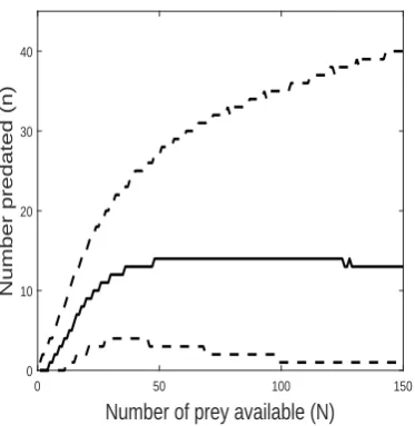
Marginal histograms of the two sets of prior samples are shown in Figure 2. The approx-imate prior predictive median and 95% interval of the number of prey predated from the BBG model are shown in Figure 3.
With the prior samples in hand, we perform our robust optimal design procedure for the remaining 78 observations in the experiment. To avoid any problems with local optima, we run our exchange method on each utility function 50 times, with each run using a different random seed. To assess the quality of the optimal robust designs we compare the results with: (i) the original design of Hassell et al. (1977) (proportionally sampled for a 78-point design); (ii) a locally optimal design using the MLE based on the pilot data; and
(iii) a random design that involves taking 78 prey levels from the vector (1,2, . . . ,150)
[image:12.595.98.493.449.657.2]with replacement. We use shorthand notation for each of the design approaches, which are detailed in Table 1.
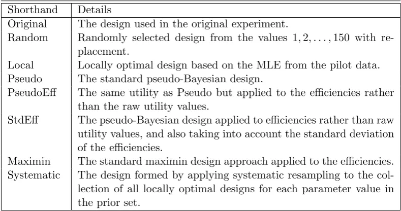
Table 1: Details for the shorthand notation that we use for each the design approaches.
Shorthand Details
Original The design used in the original experiment.
Random Randomly selected design from the values 1,2, . . . ,150 with
re-placement.
Local Locally optimal design based on the MLE from the pilot data.
Pseudo The standard pseudo-Bayesian design.
PseudoEff The same utility as Pseudo but applied to the efficiencies rather
than the raw utility values.
StdEff The pseudo-Bayesian design applied to efficiencies rather than raw
utility values, and also taking into account the standard deviation of the efficiencies.
Maximin The standard maximin design approach applied to the efficiencies.
Systematic The design formed by applying systematic resampling to the
col-lection of all locally optimal designs for each parameter value in the prior set.
5 10 15 20 25 30 0 5 10 15 20 25
(a) A a
5 10 15 20 25 30
0 5 10 15 20 25 30
(b) Ba
0 5 10 15 20 25
0 5 10 15 20 25 30 35
(c) Ab
0 5 10 15 20 25
0 5 10 15 20 25 30 35
(d) Bb
0 0.05 0.1 0.15 0.2 0.25 0.3 0 5 10 15 20 25
(e) Ac
0 0.05 0.1 0.15 0.2 0.25 0.3 0 5 10 15 20 25
(f) Bc
0 0.05 0.1 0.15 0.2 0.25 0 5 10 15 20 25 30 35 40 45
(g) Aλ
0 0.05 0.1 0.15 0.2 0.25 0 5 10 15 20 25 30 35 40 45
[image:13.595.139.459.85.738.2](h) Bλ
0 50 100 150 Number of prey available (N)
0 10 20 30 40
[image:14.595.202.389.95.287.2]Number predated (n)
Figure 3: Prior predictive distribution of the response variable (number of prey predated) for the BBG model. The solid line is the approximate prior predictive median whilst the dashed lines represent the approximate 95% prior predictive interval.
and Systematic look quite different, with a much larger spread of design points with far fewer replicates each (there are many design points with just a single replicate allocated), although there is still a heavy concentration on the lower end (between 1 to 40 prey).
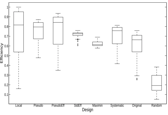
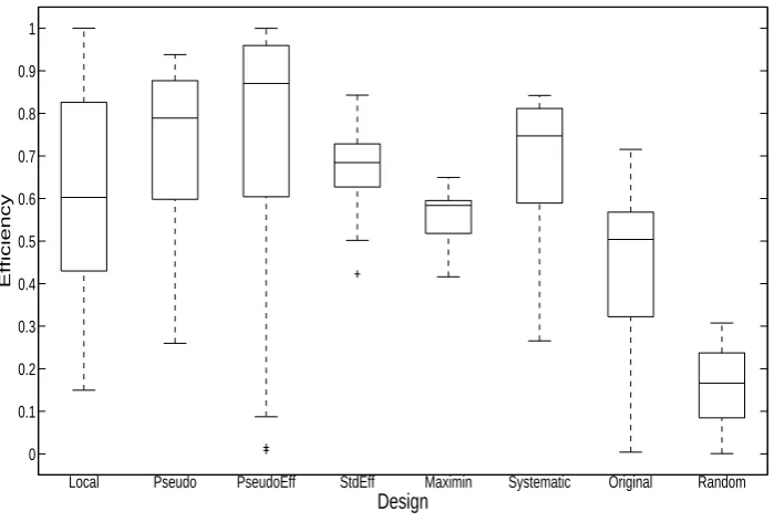
Figure 5 shows boxplots of the D-efficiencies obtained for different designs based on prior
samples A (Figure 5(a)) and prior samples B (Figure 5(b)). From both figures it is
clear that the random design performs poorly, so some thought about the experimental design, either through the use of experts, or the methods described here, or both, is very important.
It is evident that the local design is not robust to different parameter configurations, but the design selected for the original experiment in Hassell et al. (1977) was chosen sensibly, as evidenced by their respective spreads in efficiency under different parameter configurations. Figure 5(a) also shows that all of the robust utilities offer some general improvement in the efficiencies. In particular, the StdEff method seems to perform well given that it has the smallest interquartile range and that its median value is close to the highest median value. The systematic approach also appears to perform reasonably well (with results being similar to the Pseudo utility) given that it is relatively easy to calculate.
However, the efficiencies from the robust design approaches may be biased upwards since they are being assessed on the same parameter values used to obtain the designs. Thus, in Figure 5(b), we reassess the robust designs on the fresh prior samples B. It is evident that the interquartile ranges of the robust design boxplots are wider than Figure 5(a), suggesting that it is not reasonable to assess the designs based on the same parameter values used to generate them (as expected). Despite this, the results are qualitatively similar. The StdEff utility still performs well here and so does the Systematic approach relative to computational effort. The gain of using the optimal design methods over the Original design is in the order of 10 to 15% increase in the median efficiency value, with some designs (such as StdEff) also offering a tighter interquartile range.
0 20 40 60 80 100 120 140 160 0 2 4 6 8 10 12 14 16 (a) Original
0 20 40 60 80 100 120 140 160 0 5 10 15 20 25 30 35 40 (b) Local
0 20 40 60 80 100 120 140 160 0 2 4 6 8 10 12 14 16 (c) Pseudo
0 20 40 60 80 100 120 140 160 0 2 4 6 8 10 12 14 16 (d) PseudoEff
0 20 40 60 80 100 120 140 160 0 2 4 6 8 10 12 14 16 (e) StdEff
0 20 40 60 80 100 120 140 160 0 2 4 6 8 10 12 14 16 (f) Maximin
0 20 40 60 80 100 120 140 160 0 2 4 6 8 10 12 14 16 (g) Systematic
[image:15.595.140.461.84.719.2]0 20 40 60 80 100 120 140 160 0 2 4 6 8 10 12 14 16 (h) Random
0 0.1 0.2 0.3 0.4 0.5 0.6 0.7 0.8 0.9 1
Local Pseudo PseudoEff StdEff Maximin Systematic Original Random
Design
Efficiency
(a) prior samples A
0 0.1 0.2 0.3 0.4 0.5 0.6 0.7 0.8 0.9 1
Local Pseudo PseudoEff StdEff Maximin Systematic Original Random Design
Efficiency
[image:16.595.122.475.158.654.2](b) prior samples B
data can be generally less informative than binomial data. Such variability might make it difficult to discriminate between the performance of the different robust approaches. To investigate this further, we also applied the same optimal design methods to the Binomial-Gompertz (BG) functional response model equation (Fenlon and Faddy, 2006). From Figure 6, we can see that there is a more noticeable difference now between the vari-ous methods. Examining the sample B box plot in particular, StdEff exhibits a very tight interquartile range, as well as the best ‘worst case’ scenario (lowest efficiency value). Maximin offers a similarly tight interquartile range, but unfortunately with a much lower median efficiency. PseudoEff offers much higher efficiency values than Original in general, although its performance is more variable. Systematic also shows a steady 10% increase in median efficiency compared to the Original method, with a similar spread. In this model, we suggest that StdEff and Pseudo offer compelling alternatives to the Original design, depending on whether the experimenter is interested in higher or more reliable efficiency outcomes.
0.1 0.2 0.3 0.4 0.5 0.6 0.7 0.8 0.9 1
Local Pseudo PseudoEff StdEff Maximin Systematic Original Random
Design
[image:17.595.122.473.299.539.2]Efficiency
Figure 6: Boxplots of the D-efficiencies obtained for different designs based on prior sam-ples B. The results are based on the BG model.
3.2 Case Study II
In this section we consider the experiment of Papanikolaou et al. (2016a), which was
con-cerned with the functional response of a widespread ladybird beetle (Propylea
quatuordec-impunctata L.) to its insect prey (Aphis fabae Scopoli). For details on the experimental
conditions, see Papanikolaou et al. (2016a). 60 observations were taken with each ob-servation having one of the following initial number of prey, N = {4,8,16,32,64,128}. Similarly to the previous case study, we consider an experimentalist wishing to re-design this experiment where the primary objective is to accurately estimate the parameters of the following model:
(i) population dynamics are modelled using Holling’s disc equation in which it is
as-sumed that there is no prey depletion (i.e. setting N =N0 in 1). This assumption
produces an expected number of prey attacked given by
E[n] = N − {N−[rN T /(1 +rThN)]}
N ,
where T = 24 hours for this experiment.
(ii) the variability in the data is captured using a beta-binomial model as in (3). The
model parameter is thusθ ={r, Th, λ}. We refer to this as the Beta-Binomial-Holling
(BBH) model.
For this example, the pilot data consists of two observations taken randomly from the dataset at each prey level. The prior distribution on each of the parameters before pilot data collection is set to an exponential distribution with mean 100, with all parameters
independenta priori. We run 100,000 iterations of MCMC from a suitable starting value
and thin the chain by a factor of 1,000, producing 100 roughly independent samples from the posterior conditional on the pilot data. We then use these as prior distribution samples to form an optimal robust design for the remaining 48 observations.
Efficiency boxplots (based on a fresh set of prior samples not used in the optimal design procedure) for all the robust design approaches outlined in this paper are shown in Figure 7, along with a random design, the original design, and a local MLE design for comparison purposes. Each design is illustrated in the histograms in Figure 8. The BBH efficiency plots in Figure 7 are qualitatively similar to the BBG and BG model results: StdEff and Maximin have produced the smallest interquartile range whilst still having higher median values than the original design, and all the robust design approaches offer clear improvements relative to the original design.
4
Discussion
In this paper, we have demonstrated the application of optimal design methodology to functional response experiments. In the process, we have developed some additional ap-proaches for determining designs that are robust to parameter uncertainty, which could be applied in other design problems.
0 0.1 0.2 0.3 0.4 0.5 0.6 0.7 0.8 0.9 1
Local Pseudo PseudoEff StdEff Maximin Systematic Original Random
Design
[image:19.595.123.473.102.338.2]Efficiency
Figure 7: Boxplots of the D-efficiencies obtained for different designs based on prior sam-ples B. The results are based on the BBH model.
computationally efficient. It would also be straightforward to extend the idea to cases where there is model uncertainty. This would involve taking prior parameter samples from each of the models, and then performing a local optimal design for each parameter value. After concatenating all local optimal designs, a design that is robust to model and parameter uncertainty can be obtained by performing an appropriate clustering of the concatenation.
Furthermore, the clustering idea could be used in fully Bayesian design. Whilst in clas-sical design the utility function is often a functional of the FIM, in Bayesian design the utility is often a functional of the posterior distributed computed from future datasets that might arise from the proposed experimental design. An advantage of the Bayesian approach is that its utility is based on a posterior functional, and so does not rely on an asymptotic approximation that the FIM-based utility does. In a Bayesian optimal design procedure, the posterior distribution needs to be computed many times leading to a high computational cost (see Ryan et al. (2016) for the computational challenges in Bayesian design). Thus methods for reducing computation are sought. We plan to investigate the clustering approach for fully Bayesian design in further research.
Here we focussed on optimising the prey levels for a fixed number of experimental obser-vations. However, our optimisation method could be modified to handle the constraint where the total number of prey available for the experiment is fixed instead.
0 50 100 150 200 250 0 5 10 15 20 25 30 (a) Original
0 50 100 150 200 250 0 5 10 15 20 25 30 (b) Local
0 50 100 150 200 250 0 5 10 15 20 25 30 (c) Pseudo
0 50 100 150 200 250 0 5 10 15 20 25 30 (d) PseudoEff
0 50 100 150 200 250 0 5 10 15 20 25 30 (e) StdEff
0 50 100 150 200 250 0 5 10 15 20 25 30 (f) Maximin
0 50 100 150 200 250 0 5 10 15 20 25 30 (g) Systematic
[image:20.595.138.458.90.715.2]0 50 100 150 200 250 0 5 10 15 20 25 30 (h) Random
are met (instead of fixing the total number of samples up front). The drawback of the se-quential design process is that it takes a longer time to conduct the experiment. However, we suggest that it is worth considering depending on the logistics of the experiment.
In conclusion, we have developed effective robust optimal design methods for integer-based experimental scenarios. We successfully applied the methods to a novel application in functional response experiments.
Data Accessibility
Matlab code and data to implement our methods for the first case study is available at http://www.runmycode.org/companion/view/2708.
Funding
CCD was supported by an Australian Research Council’s Discovery Early Career Re-searcher Award funding scheme (DE160100741). NEP acknowledges financial support from the “Foundation for Education and European Culture” under a postdoctoral re-search grant (2016-2018).
Acknowledgments
The authors are grateful to James McGree for comments on an earlier draft. The authors also thank two anonymous referees whose suggestion led to improvements in this paper.
References
Accolla, C., Nerini, D., Maury, O., and Poggiale, J.-C. (2015). Analysis of functional
response in presence of schooling phenomena: An IBM approach. Progress in
Oceanog-raphy, 134:232–243.
Casas, J. and Hulliger, B. (1994). Statistical analysis of functional response experiments.
Biocontrol Science and Technology, 4(2):133–145.
Chaloner, K. and Verdinelli, I. (1995). Bayesian experimental design: A review. Statistical
Science, pages 273–304.
Cook, R. D. and Nachtsheim, C. J. (1980). A comparison of algorithms for constructing
exact D-optimal designs. Technometrics, 22(3):315–324.
Cook, R. D. and Wong, W. K. (1994). On the equivalence of constrained and compound
optimal designs. Journal of the American Statistical Association, 89(426):687–692.
Dette, H. (1997). Designing experiments with respect to ’standardized’ optimality criteria.
Journal of the Royal Statistical Society: Series B (Statistical Methodology), 59(1):97–
Dick, J. T., Alexander, M. E., Ricciardi, A., Laverty, C., Downey, P. O., Xu, M., Jeschke, J. M., Saul, W.-C., Hill, M. P., Wasserman, R., Barrios-ONeill, D., Weyl, O. L. F.,
and Shaw, R. H. (2017). Functional responses can unify invasion ecology. Biological
Invasions, 19(5):1667–1672.
Dror, H. A. and Steinberg, D. M. (2006). Robust experimental design for multivariate
generalized linear models. Technometrics, 48(4):520–529.
Drovandi, C. C., McGree, J. M., and Pettitt, A. N. (2014). A sequential Monte Carlo to
incorporate model uncertainty in Bayesian sequential design. Journal of Computational
and Graphical Statistics, 23(1):3–24.
Fedorov, V. V. (1972). Theory of optimal experiments. Elsevier.
Fenlon, J. S. and Faddy, M. J. (2006). Modelling predation in functional response.
Eco-logical Modelling, 198(1):154–162.
Gotwalt, C. M., Jones, B. A., and Steinberg, D. M. (2009). Fast computation of designs
robust to parameter uncertainty for nonlinear settings. Technometrics, 51(1):88–95.
Hassell, M., Lawton, J., and Beddington, J. (1977). Sigmoid functional responses by
invertebrate predators and parasitoids. The Journal of Animal Ecology, 46(1):249–262.
Holling, C. S. (1959). Some characteristics of simple types of predation and parasitism.
The Canadian Entomologist, 91(07):385–398.
Hossie, T. J. and Murray, D. L. (2016). Spatial arrangement of prey affects the shape
of ratio-dependent functional response in strongly antagonistic predators. Ecology,
97(4):834–841.
Jeschke, J. M., Kopp, M., and Tollrian, R. (2002). Predator functional responses:
dis-criminating between handling and digesting prey. Ecological Monographs, 72(1):95–112.
Oaten, A. and Murdoch, W. W. (1975). Functional response and stability in predator-prey
systems. The American Naturalist, 109(967):289–298.
Papanikolaou, N., Williams, H., Demiris, N., Preston, S., Milonas, P., and Kypraios, T. (2016a). Bayesian inference and model choice for holling’s disc equation: a case study
on an insect predator-prey system. Community Ecology, 17(1):71–78.
Papanikolaou, N. E., Demiris, N., Milonas, P. G., Preston, S., and Kypraios, T. (2016b). Does mutual interference affect the feeding rate of aphidophagous coccinellids? A
mod-eling perspective. PLOS ONE, 11(1):e0146168.
Papanikolaou, N. E., Milonas, P. G., Demiris, N., Papachristos, D. P., and Matsinos,
Y. G. (2014). Digestion limits the functional response of an aphidophagous
coc-cinellid (Coleoptera: Coccoc-cinellidae). Annals of the Entomological Society of America,
107(2):468–474.
Ryan, E., Drovandi, C. C., and Pettitt, A. N. (2015). Fully Bayesian experimental design
for pharmacokinetic studies. Entropy, 17(3):1063–1089.
Ryan, E. G., Drovandi, C. C., McGree, J. M., and Pettitt, A. N. (2016). A review of
modern computational algorithms for Bayesian optimal design. International Statistical
Stenseth, N. C., Shabbar, A., Chan, K.-S., Boutin, S., Rueness, E. K., Ehrich, D., Hurrell, J. W., Lingjærde, O. C., and Jakobsen, K. S. (2004). Snow conditions may create an
invisible barrier for lynx. Proceedings of the National Academy of Sciences of the United
States of America, 101(29):10632–10634.
Trexler, J. C., McCulloch, C. E., and Travis, J. (1988). How can the functional response
best be determined? Oecologia, 76(2):206–214.
Walter, ´E. and Pronzato, L. (1987). Optimal experiment design for nonlinear models
sub-ject to large prior uncertainties. American Journal of Physiology-Regulatory, Integrative
and Comparative Physiology, 253(3):R530–R534.
Weterings, R., Umponstira, C., and Buckley, H. L. (2015). Density-dependent allometric
functional response models. Ecological Modelling, 303:12–18.
Woods, D. C., Lewis, S. M., Eccleston, J. A., and Russell, K. (2006). Designs for
gen-eralized linear models with several variables and model uncertainty. Technometrics,
48(2):284–292.
Zimmermann, B., Sand, H., Wabakken, P., Liberg, O., and Andreassen, H. P. (2015). Predator-dependent functional response in wolves: from food limitation to surplus
Appendix
For simplicity we only provide instructions on how to obtain the expression for the first diagonal element of the FIM. The process for the other elements follows in a similar way.
Further, this is only shown for a single design variable N since the FIM for a potential
design N can be obtained by summing the FIMs for the individual observations. The
log-likelihood for a single observation is given by
l(n;N, α, β) = log
N n
+ log Γ(n+α) + log Γ(N−n+β)−log Γ(N +α+β)−
log Γ(α)−log Γ(β) + log Γ(α+β). (11)
Recall that
µ= α
α+β =
a
N(e
−bexp(−cN)−e−b) and
λ= 1
α+β,
so that α = µ/λ and β = (1−µ)/λ. Take, for example, the term log Γ(N +α +β).
Differentiating this with respect toagives
∂
∂alog Γ(N +α+β) =ψ
(0)(N+α+β)
∂α
∂a +
∂β ∂a
,
where
∂α
∂a =
∂α ∂µ
∂µ
∂a and
∂β
∂a =
∂β ∂µ
∂µ
∂a.
The partial derivatives on the right hand side of the above are easy to obtain. A similar
process needs to be repeated for each of the log Γ(·) terms in (11). The second derivative
of log Γ(N+α+β) involves the use of the product rule, repeated application of the chain
rule and also the polygamma function of order 1,ψ(1)(·).
The first diagonal element of the OIM is given by
O(n;θ,N)1,1 =−
∂2`(n;θ,N)
∂a2 .
To obtain the corresponding component of the FIM, the expected value with respect to
nmust be calculated. We note that the OIM component above does involve expectations
with respect to each individual n for a variety of non-linear functions of n. If we denote
E[g(n)] =
N X
i=1
g(i)p(n=i;N),
wherep(n=i;N) is the probability mass function of the beta-binomial distribution with
N being the number of trials (the corresponding prey level that will be used). There is
no analytical solution for this expectation so it must be evaluated numerically. Thus the
computational cost of evaluating a single entry of the FIM is of the orderK×max(N).
In practice, we use the symbolic toolbox in Matlab to evaluate the necessary derivatives for the FIM as shown below. These expressions can be converted into Matlab code with some
manual adjustments. Any terms involving non-linear functions ofnneed to replaced with
code to compute the expected value as shown above. If there are some terms that appear several times in the derivatives for the FIM the code can be accelerated by computing such quantities once and re-using them.
%% Calculation of the partial derivatives for the BBG model
% a,b,c are the parameters from Gompertz eqn
% alpha and beta are from the beta-binomial function % d is the overdispersion parameter of the beta-binomial
syms N n a b c d alpha beta;
mu = (a/N)*(exp(-b*exp(-c*N))-exp(-b));
alpha = mu/d; beta = (1 - mu)/d;
% define the loglikelihood equation
bbLL = (log(factorial(N)) - log(factorial(n)) - log(factorial(N-n))... + log(gamma(n+alpha)) + log(gamma(N-n+beta)) - log(gamma(N+alpha+beta))... + log(gamma(alpha+beta)) - log(gamma(alpha)) - log(gamma(beta)));
% first partial derivatives bbLLa = diff(bbLL,a);
bbLLb = diff(bbLL,b); bbLLc = diff(bbLL,c); bbLLd = diff(bbLL,d);
% second partial derivatives bbLLaa = diff(bbLLa,a); bbLLbb = diff(bbLLb,b); bbLLcc = diff(bbLLc,c); bbLLdd = diff(bbLLd,d);
bbLLad = diff(bbLLa,d);
bbLLbc = diff(bbLLb,c); bbLLbd = diff(bbLLb,d);