Monetary and macroprudential policies under fixed and variable interest rates

Monetary and Macroprudential Policies under Fixed and Variable

Interest Rates

Margarita Rubio

University of Nottingham

September 2016

Abstract

In this paper, I analyze the ability of monetary policy to stabilize both the macroeconomy and …nancial markets under two di¤erent scenarios: …xed and variable-rate mortgages. I develop and solve a New Keynesian dynamic stochastic general equilibrium model (DSGE) that features a housing market and a group of constrained individuals who need housing collateral to obtain loans. A given share of constrained households borrows at a variable rate, while the rest borrow at a …xed rate. I consider two alternative ways of introducing a macroprudential approach to enhancing …nancial stability: one in which monetary policy, using the interest rate as an instrument, responds to credit growth; and a second one in which the macroprudential instrument is instead the loan-to-value ratio (LTV). The results show that when rates are variable, a countercyclical LTV rule performs better in stabilizing …nancial markets than monetary policy. However, when rates are …xed, even though monetary policy is less e¤ective in stabilizing the macroeconomy, it does a good job in promoting …nancial stability.

Keywords: …xed/variable-rate mortgages, monetary policy, macroprudential policy, LTV, housing market, collateral constraint

JEL Codes: E32, E44, E52

"The explicit incorporation of macroprudential considerations in the nation’s framework for …nancial

oversight represents a major innovation in our thinking about …nancial regulation [:::] This new

direc-tion is constructive and necessary, I believe, but it also poses considerable conceptual and operadirec-tional

challenges in its implementation." Ben Bernanke, May 5, 2011.

1

Introduction

In recent years, especially during the period of the Great Moderation, monetary policy was seen as a very powerful tool for stabilizing the economy. However, in the aftermath of the crisis, new experiences have revealed that this statement is not true for all cases nor in all circumstances. First of all, the e¤ectiveness of monetary policy may depend on structural factors in the economy. In particular, there may be institutional features, especially in housing markets, that are country speci…c and that may a¤ect the optimal conduct of policies. One source of heterogeneity, which can be crucial, is the structure of mortgage contracts. Mortgage contracts in an economy can involve either a …xed or variable rate, and the proportion of each type of mortgage varies from country to country. The link between the policy rate and …xed rates is weaker, because the latter are more connected to longer-term rates, and thus, in this case, monetary policy is less e¤ective.1 On the other hand, with the crisis, policy and academic discussions have focused on how to ensure a more stable …nancial system: a macroprudential approach to prevent situations in which problems in the …nancial sector are transmitted to the real sectors of the economy and vice versa. It is debatable whether monetary policy alone can achieve this goal; it may need the help of other tools that help avoid excessive credit growth. The following question remains. Does the mortgage structure of the economy a¤ect the ability of monetary policy to enhance …nancial stability?

In this paper, I try to shed some light on this issue. I analyze the ability of monetary policy to stabilize …nancial markets under two di¤erent scenarios: when the prevalent mortgage rate in the economy is variable and when it is …xed. Recent literature shows that the e¤ectiveness of monetary policy in stabilizing the macroeconomy is reduced when rates are …xed. Nevertheless, the literature is silent about whether this feature has an impact on the potential of monetary policy to promote …nancial stability.

There is evidence of di¤erent cross-country mortgage contracts. While …xed-rate mortgages

predom-1_{See Rubio (2011) or Brzoza-Brzezina (2014) for theoretical models that show that …xed-rate contracts imply less e¤ective}

inate in the US, the majority of consumers borrow at a variable rate in Canada and Australia. Within European countries, we have striking di¤erences such that the vast majority of consumers in the United Kingdom and Spain have variable-rate mortgages, as opposed to Germany and France where most mort-gage rates are …xed (see Table A1 in the Appendix). Rubio (2011) and Calza et al. (2013) show that the structure of mortgage contracts has important implications for the transmission of monetary policy in the sense that policy rate changes are less e¤ective when the mortgage rate is …xed. However, these papers do not touch upon the issue of whether having …xed- or variable-rate mortgages may also a¤ect …nancial stability and the optimal design of macroprudential policies.

In this paper, I build a new Keynesian dynamic stochastic general equilibrium model with housing, collateral constraints, and …xed- and variable-rate mortgages to study how the mortgage structure in an economy a¤ects the optimal design of both monetary and macroprudential policies. In the model, there are three types of consumers: savers, variable-rate borrowers and …xed-rate borrowers. Borrowers need collateral in order to access credit markets, which are more or less tight depending on the loan-to-value ratio (LTV). Monetary policy is conducted by the central bank. For the macroprudential policies, I consider two options: one where they are conducted by the central bank with the interest rate as the instrument, and a second one in which there is a macroprudential regulator that uses a countercyclical rule for the LTV as a macroprudential tool.

As this is a microfounded model, it is appropriate to study welfare-related issues. In this setting, there are several channels that a¤ect welfare and that are dependent on mortgage contracts. In new Keynesian models with collateral constraints, there are two types of distortions: sticky prices and credit frictions. Savers prefer policies that alleviate the …rst distortion, because they own the …rms. They are better o¤ in a scenario with price stability, the goal of monetary policy. On the contrary, borrowers’ welfare increases when the credit friction distortion is minimized. Then, borrowers may prefer situations that generate in‡ation or policies that enhance …nancial stability, namely macroprudential ones. However, these mechanisms may di¤er depending on whether the prevalent mortgage contract in the economy is a …xed or variable rate. In the variable-rate scenario, monetary policy is more stabilizing because there is a one-for-one link between the policy rate and the borrowing rate. With respect to macroprudential policies, their e¤ectiveness will also depend on whether the economy has …xed or variable rates, because their interaction with monetary policy will have an e¤ect on …nancial stability.

are no macroprudential policies. I …nd that having variable- or …xed-rate mortgages not only a¤ects the macroeconomic dynamics but also the …nancial side of the economy. The …xed-rate economy, has a less powerful monetary policy tool but borrowers are more exposed to changes in in‡ation and house prices, a¤ecting their …nancial capacity. Therefore, the structure of mortgage contracts should have clear implications, not only for monetary policy reaction but also for macroprudential policies that focus on …nancial stability. Then, it is relevant to study the optimal implementation of both monetary and macroprudential policies in the context of variable- and …xed-rate mortgages.

Then, I analyze how the optimality of monetary and macroprudential policies changes depending on the mortgage structure of the economy. I de…ne optimal policy as the one that maximizes total welfare. As mentioned, I consider two alternative ways of introducing macroprudential policies. First, I present a simple and automatic rule on the LTV. Following this rule, the LTV would be the instrument of the macroprudential regulator and would react to credit growth. In this way, if the economy is, for instance, entering a credit boom, the LTV will be cut, thus restricting credit in the economy and avoiding excessive credit growth. This rule, which resembles a Taylor rule for monetary policy, serves as a proxy for the macroprudential instruments that have been used by some institutions.2 Alternatively, I consider including credit growth in the interest-rate rule of the central bank. In this way, the monetary authority would have one instrument, the interest rate, to take care of two objectives: macroeconomic and …nancial stability.

The results show that macroprudential policies increase welfare regardless of the mortgage structure prevalent in the economy. Nevertheless, when mortgages are variable rate, an LTV rule combined with monetary policy is preferable to including credit variables in the interest-rate rule. When rates are …xed, using the interest rate as an instrument both for monetary and macroprudential policy delivers higher welfare and stability than having two separate instruments. Interestingly for the …xed-rate case, in which monetary policy is less e¤ective in stabilizing the macroeconomy, it is a more powerful tool for stabilizing the …nancial system. Sticky prices introduce a …rst distortion in the economy that can be …xed through monetary policy. However, for the …xed rate case, a simple Taylor rule responding to in‡ation and output is not able to e¤ectively …x this …rst distortion. The collateral constraint is introducing an extra distortion that can be …xed by making the regulator respond to credit variables. When credit variables

2

are introduced in the Taylor rule, it becomes a more powerful tool because of the volatility of credit with respect to the other two variables and because of the indirect e¤ects that this will have on house prices. This is indeed an example of a theory of second best, given the distortion that the collateral constraint is introducing.

This paper relates to di¤erent strands of the literature. First, it introduces heterogeneity in mortgage contracts in the spirit of Rubio (2011), Calza et al. (2013) and Garriga et al. (2015). However, those studies restrict themselves to the e¤ects of the mortgage structure on business cycles and monetary policy, without analyzing the implications for macroprudential policies. Second, it is close to the recent macroprudential literature. On the one hand, it relates with papers in which macroprudential policies interact with monetary policy as in Kannan et al. (2012), Rubio and Carrasco-Gallego (2014), and Angelini et al. (2014). However, none of the above mentioned papers examine how …xed- and variable-rate mortgages a¤ect the implementation of macroprudential policies nor a¤ect …nancial stability. On the other hand, my paper also explores whether monetary and macroprudential policies should be conducted by the same regulator using only one instrument responding to two target variables or two regulators with two di¤erent instruments. Following the same line, Beau et al. (2012) claim that it is preferable to have a combination of separate objectives for monetary and macroprudential policies. Rubio and Carrasco-Gallego (2015) also …nd that monetary policy should focus on price stability, while macroprudential policy should have …nancial stability as an instrument. Kannan et al. (2012) experiment with an augmented Taylor rule and an LTV rule as well and …nd that the results depend on the source of the shock considered. In my paper, I …nd that having two separate instruments is preferred in the case of variable-rate mortgages but the augmented Taylor rule delivers higher welfare when rates are …xed.

The paper continues as follows. Section 2 explains the basic model I build for the analysis and its dynamics. Section 3 shows the modeling of the macroprudential policies. Section 4 analyzes the normative implications of introducing macroprudential policies and displays the optimal monetary and macroprudential policy mix. Section 5 presents the conclusions. The Appendix contains tables on the empirical evidence mentioned above, sensitivity analyses, extra graphs and model derivations.

2

The Baseline Model

Firms set prices subject to Calvo (1983)-Yun (1996) nominal rigidity. The monetary authority sets interest rates endogenously, in response to in‡ation and output, following a Taylor rule.

2.1 The Consumer’s Problem

There are three types of consumers: unconstrained consumers, constrained consumers who borrow at a variable rate, and constrained consumers who borrow at a …xed rate. Constrained individuals need to collateralize their debt repayments in order to borrow from the …nancial intermediary. Interest payments for both mortgages and loans cannot exceed a proportion of the future value of the current house stock. In this way, the …nancial intermediary ensures that borrowers are going to be able to ful…ll their debt obligations next period. As in Iacoviello (2005), I assume that constrained consumers are more impatient than unconstrained ones. This assumption ensures that the borrowing constraint is binding, so that constrained individuals do not save and wait until they have the funds to self-…nance their consumption. This generates an economy in which households divide into borrowers and savers. Furthermore, borrowers are split into two groups: those who borrow at a …xed rate and those who borrow at a variable rate. The proportion of each type of borrower is …xed and exogenous. All households derive utility from consumption, and housing services are assumed proportional to the housing stock and leisure.

2.1.1 The Financial Intermediary

Consider a …nancial intermediary that accepts deposits from savers, and extends both …xed- and variable-rate loans to borrowers.3 I assume a competitive framework, and thus the intermediary takes the variable-interest rate as given. The pro…ts of the …nancial intermediary are de…ned as:

Ft= Rt 1bcvt 1+ (1 )Rt 1bcf_{t 1} Rt 1but 1; (1)

where Ft represents the pro…ts of the …nancial intermediary, is the proportion of variable rates, Rt 1

is the gross policy rate set by the central bank, andbcv_{t 1} andbcf_{t 1} are one-period variable- and …xed-rate mortgages, respectively.4 bu_{t 1} represent deposits.

In equilibrium, aggregate borrowings and savings must be equal, that is:

3

In countries where …xed-rate mortgages are most extensively used, …nancial intermediaries pass on the loans to investors with long-term liabilities (such as pension funds and life-insurance companies). Short-term deposits are predominantly used to …nance mortgages in countries where variable-rate mortgages are commonly used. These institutional features are beyond the scope of this paper.

bcv_t + (1 )bcf_t =bu_t: (2)

Substituting(2) into(1), we obtain:

Ft= (1 )bcft 1 Rt 1 Rt 1 . (3)

In order for the two types of mortgage to be o¤ered, the …xed interest rate has to be such that the intermediary is indi¤erent between lending at a variable or …xed rate.5 Hence, the expected discounted pro…ts that the intermediary obtains by lending new debt in a given period at a …xed interest rate must be equal to the expected discounted pro…ts the intermediary would obtain by lending it at a variable rate:6

E

1 X

i= +1

i

;iR =E

1 X

i= +1

i

;iRi 1; (4)

where t;i = C_tu

C_tu_+i is the unconstrained consumer-relevant discount factor. As the …nancial

interme-diary is owned by the savers, their stochastic discount factor is applied to the …nancial intermeinterme-diary’s problem.7 Note that, as stated previously, variable-rate debt is one period but the portion of new debt acquired at a …xed rate is associated with a long-term contract.8 _{As the agent is in…nitely lived, the}

…nancial intermediary considers an in…nitely lasting maturity in these calculations.9 We can obtain the equilibrium value of the …xed rate in period from expression(4):

R =

E P1

i= +1

i

;iRi 1

E P1

i= +1

i ;i

. (5)

Equation (5)states that, for every new debt issued at date , there is a di¤erent …xed interest rate

5_{The steady-state …xed rate equals the steady-state variable rate and therefore the steady state of the model is not}

a¤ected by this speci…cation.

6

The …xed-rate loan is priced following this nonarbitrage condition, not by applying the prices of zero-coupon bonds to the future cash ‡ows from the new loan.

7

Note that there is no di¤erence between having the …nancial intermediary as a separate agent or putting these decisions with the patient household.

8

The long-term contract relates primarily to the interest rate, rather than the debt being explicitly amortized.

9_{Calza et al. (2010) also develop a model in which the …nancial intermediary o¤ers …xed- and variable-rate mortgages.}

that has to be equal to a discounted average of future variable interest rates. Note that this is not a condition on the stock of debt, but on the new amount obtained in a given period. New debt at a given point in time is associated with a di¤erent …xed interest rate. Both the …xed interest rate in period and the new amount of debt in period are …xed for all future periods. However, the …xed interest rate varies with the date the debt was issued, so that in every period there is a new …xed interest rate associated with new debt in this period. If we consider …xed-rate loans to be long term, the …nancial intermediary obtains interest payments every period from the whole stock of debt, not only from the new debt. Hence, we can de…ne the aggregate …xed interest rate as being the one the …nancial intermediary e¤ectively charges every period for the whole stock of mortgages. This aggregate …xed interest rate is a function of all past …xed interest rates on past debt, together with the current period equilibrium …xed interest rate on the new debt. Therefore, the e¤ective …xed interest rate that the …nancial intermediary charges for the stock of …xed-rate debt every period is:

Rt=

8 > < > :

Rt 1bcft 1+Rt b cf

t b

cf

t 1

bcf_t ifb

cf t > b

cf

t 1

Rt 1 ifbcft b cf t 1 9 > = >

;. (6)

Equation(6)states that the …xed interest rate that the …nancial intermediary is actually charging today is an average of what it charged last period for the previous stock of mortgages and what it charges this period for the new amount.10 In the case that there is no new debt, the …xed interest rate will be equal to last period’s.11 _{Then, in the same way that variable rates are revised every period, …xed rates}

are revised by including the new optimal …xed interest rate for the new debt originated in this period. Importantly, this assumption is not crucial for the results. Both R and Rt are practically una¤ected

by interest rate shocks.12 This assumption is a way to make the model compatible with the fact that …xed-rate loans are not one-period assets but are longer-term ones.13 Therefore, even though strictly speaking all mortgages are one-period loans in this model, equation(6)makes …xed-rate loans long-term ones. In this case, if there is new borrowing, this will add to the existing stock of loans at a new optimal

1 0_{This expression can be interpreted in a similar way as in Calza et al. (2010). In their model, the …xed rate loan is}

repaid in two periods. Here, while the contract is of in…nite maturity, I also divide payments into two blocks: the new payments made this period for new loans and the payments for the old loans.

1 1

Note that, if Rt > Rt, remortgaging to a lower Rt is not allowed in the model. The agent cannot repay the most

expensive mortgages …rst either.

1 2

When the model is log-linearized, the non-linearity disappears because the …xed interest rate does not move from the steady-state interest rate. Please see the Appendix for details.

1 3_{In the real world, variable-rate mortgages are also long-term loans. That is, both loans are amortized over a long}

…xed interest rate. If there is no new debt, the interest rate that is charged for the existing stock does not change. The contract is set at a speci…c point in time and lasts for as many periods as there is no new debt. If there is new debt, a new …xed interest rate is calculated and an average interest rate composed of the past interest rate and this new interest rate will be applied to the whole stock of debt. This new interest rate will also last for as many periods as there is no new debt.

As noted above, any pro…ts from …nancial intermediation are rebated to the unconstrained consumers every period. Even if the …nancial intermediary is competitive and pro…ts are expected to be zero, if there is a shock at a given point in time, the fact that only the variable interest rate is directly a¤ected can generate nonzero pro…ts.

2.1.2 Unconstrained Consumers (Savers)

Unconstrained consumers maximize:

max E0

1 X

t=0

t _lnCu

t +jtlnHtu

(Lu_t)

, (7)

where the superscript u stands for "unconstrained," E0 is the expectation operator, 2 (0;1) is the

discount factor, and C_tu, H_tu and Lu_t are consumption at t, the stock of housing and hours worked, respectively; 1=( 1) is the labor supply elasticity, > 0. jt represents the weight of housing in the

utility function. I assume that log(jt) = log(j) +uJ t; where uJ t follows an autoregressive process. A

shock to jt represents a shock to the marginal utility of housing. These shocks directly a¤ect housing

demand and therefore can be interpreted as a proxy for exogenous disturbances to house prices. The budget constraint is:

C_tu+qtHtu+but qtHtu 1+wutLut +

Rt 1but 1

t

+F_tv+S_tv; (8)

where qt is the real housing price and wtu is the real wage for unconstrained consumers who can buy

houses or sell them at the current price qt. I assume zero housing depreciation for simplicity. As we

will see, this group will choose not to borrow at all; they are the savers in this economy. bu_t is the amount they save. They receive interestRt 1 for their savings. t is in‡ation in periodt. Stand Ft are

The …rst-order conditions for this unconstrained group are:

1

C_tu = Et

Rt

t+1C_tu₊₁

, (9)

wu_t = (Lu_t) 1C_tu; (10)

jt H_tu =

1

C_tuqt Et 1

C_tu₊₁qt+1: (11)

Equation (9) is the Euler equation for consumption, equation (10) is the labor-supply condition, and equation (11) is the Euler equation for housing. This states that the bene…ts from consuming housing must be equal to the costs at the margin.

2.1.3 Constrained Consumers (Borrowers)

Constrained consumers are of two types: those who borrow at a variable rate and those who do so at a …xed rate. The di¤erence between them is simply the interest rate they face. The …xed-rate borrower faces Rt, set by the …nancial intermediary, whereas the variable-rate counterpart faces Rt, set by the

central bank. The proportion of variable-rate consumers is …xed and exogenous and equal to ₂[0;1].14

Constrained and unconstrained consumers are di¤erent in the way they discount the future. Con-strained consumers are more impatient than unconCon-strained ones. I assume that conCon-strained consumers face a limit on the debt they can acquire. The maximum amount they can borrow is proportional to the value of their collateral, in this case the stock of housing. That is, the debt repayment next period cannot exceed a proportion of tomorrow’s value of today’s stock of housing:

Et Rt

t+1

bcv_t ktEtqt+1Htcv; (12)

Et Rt

t+1

bcf_t ktEtqt+1Htcf; (13)

1 4

where(12)represents the collateral constraint for the variable-rate constrained consumer and(13)is the constraint for the …xed-rate one.15 The superscriptcvstands for "constrained variable," whilecf stands for "constrained …xed." kt represents a proxy for the LTV and, as we will see, it is the instrument of

the macroprudential authority. As we have seen with the problem of the …nancial intermediary, Rt is

an aggregate interest rate that contains information on all the past …xed interest rates associated with past debt. Each period, this aggregate interest rate is updated with a new interest rate linked to the new amount of debt originated in that period.

Without loss of generality, I present the problem for the variable-rate borrower, because the one for the …xed-rate borrower is symmetric. Variable-rate borrowers maximize their lifetime utility function:

max E0

1 X

t=0

et _lnCcv

t +jtlnHtcv

(Lcv_t )

, (14)

subject to the budget constraint:

C_tcv+qtHtcv+

Rt 1bcvt 1

t

qtHtcv1+wtcvLcvt +bcvt ; (15)

and (12), the collateral constraint.16 Note that variable-rate borrowers repay all debt every period and acquire new debt at the current new interest rate. This assumption implies that the interest rate on variable-rate mortgages is revised every period for the whole stock of debt and changed according to the policy rate.17 In order to make the problem for …xed-rate borrowers symmetric and analogous to the existing models with borrowing constraints, I assume the same debt-repayment structure for this type of borrower. Obviously, …xed-rate contracts are not revised every period. However, to make the model more realistic but still tractable, the …xed interest rate will be such that a revised …xed rate will be applied only on new debt, keeping constant the interest rate applied to existing debt. In this way, I reconcile the structure of the model with the fact that …xed-rate contracts are long term.18

1 5

Garriga et al. (2005) and Alpanda et al. (2014) take a slightly di¤erent approach for their borrowing constraint. This strand of the literature di¤erentiates the e¤ects of policies that apply only to new lending as opposed to all existing mortgage debt. The constraint on borrower households is imposed on the ‡ow rather than the stock of household debt, and new mortgage loans are modeled as …xed rate. This feature captures the notion that a signi…cant share of new mortgage loans in the real world are adjustable-rate loans, and some …xed-rate mortgages are re…nanced before the end of their amortization period. With this speci…cation, an increase in debt in this period leads to a tightening of the borrowing constraint next period as well. However, with full amortization, both borrowing constraints would be equivalent.

1 6

We will see from the …rm’s problem thatwcvt =wtcf =w c t:

1 7_{This assumption is consistent with reality, in which variable interest rates are revised very frequently and changed}

according to an interest-rate index tied to the interest rate set by the central bank.

1 8_{Another option would be to have an overlapping generations model in which we are able to keep track of the debt issued}

As noted above, constrained consumers are more impatient than unconstrained ones, so that e< . This assumption is crucial for the borrowing constraint to be binding and therefore, for there to be both borrowers and savers in the economy.

The …rst-order conditions for variable-rate constrained consumers are:

1

C_tcv = eEt

Rt

t+1C_tcv₊₁

+ cv_t Rt; (16)

wcv_t = (Lcv_t ) 1C_tcv; (17)

jt H_tcv =

1

C_tcvqt eEt 1 C_tcv₊₁qt+1

cv

t ktEt(qt+1 t+1). (18)

These …rst-order conditions di¤er from those of the unconstrained individuals. In the case of con-strained consumers, the Lagrange multiplier on the borrowing constraint( cv_t )appears in equations(16)

and (18).19 From the Euler equation for the consumption of unconstrained consumers, we know that

R = 1= in the steady state. If we combine this result with the Euler equation for the consumption of the constrained individuals we have that cv = e =Ccv >0in the steady state. This means that the borrowing constraint holds with equality in the steady state. As we log-linearize the model around the steady state and assume that uncertainty is low, we can generalize this result to o¤-steady-state dynamics. Then, the borrowing constraint is always binding, so that constrained individuals borrow the maximum amount they are allowed to and unconstrained consumers are never in debt.20

Given the borrowing amount implied by(12)at equality, consumption of the variable-rate constrained individuals can be determined by their ‡ow of funds:

C_tcv=wcv_t Lcv_t +bcv_t +qt Htcv1 Htcv

Rt 1bcvt 1

t

; (19)

and the …rst-order condition for housing becomes:

jt Hcv t = 1 Ccv t qt

ktEt(qt+1 t+1)

Rt

eEt

1 Ccv

t+1

(1 kt)qt+1 : (20)

1 9

In the log-linearized versions of the Euler equations for both consumer types, I include a demand shock re‡ecting exogenous changes in demand. See equations (46) and (47) in the Appendix.

2 0

2.2 Firms

2.2.1 Final Goods Producers

There is a continuum of identical …nal goods producers that aggregate intermediate goods according to the production function:

Yt=

Z 1

0

Yt(z) " 1

" _dz " " 1

; (21)

where " > 1 is the elasticity of substitution between intermediate goods. The …nal good …rm chooses

Yt(z)to minimize its costs, resulting in demand of intermediate good z:

Yt(z) =

Pt(z) Pt

"

Yt: (22)

The price index is then given by:

Pt=

Z 1

0

Pt(z)1 "dz

1

" 1

: (23)

Market clearing for the …nal good requires:

Yt=Ct=Ctu+Ctc:

2.2.2 Intermediate Goods Producers

The intermediate goods market is monopolistically competitive. Following Iacoviello (2005), intermediate goods are produced according to the production function:

Yt(z) =AtLtu(z) Lct(z)

(1 )

; (24)

where ₂[0;1]measures the relative size of each group in terms of labor. This Cobb-Douglas production function implies that the labor e¤orts of constrained and unconstrained consumers are not perfect substi-tutes. This speci…cation is analytically tractable and allows for closed-form solutions for the steady state of the model. This assumption can be economically justi…ed by the fact that savers are the managers of the …rms and their wages are higher than those of the borrowers.21 Experimenting with a production

function in which labor hours for both types of consumers are substitutes leads to very similar results in terms of model dynamics. Under the Cobb-Douglas speci…cation, each household has mass one. is a constant that represents the labor-income share of the patient household and Lu_t are total hours worked by the patient household. In the alternative speci…cation, one needs to de…ne the fraction of agents in the population, assuming that ! is the fraction of savers. Then, !Lu_t represents the total hours worked by the patient household. Therefore, both speci…cations are very similar but, while represents the economic size of savers,! would correspond to their absolute size.22

At represents technology and it follows the following autoregressive process:

log (At) = Alog (At 1) +uAt; (25)

where A is the autoregressive coe¢ cient anduAt is a normally distributed shock to technology.

Labor demand is determined by:

w_tu= 1 Xt

Yt

Lu_t; (26)

wc_t = 1 Xt

(1 ) Yt Lc t

; (27)

where Xt is the markup, or the inverse of marginal cost.23

The price-setting problem for the intermediate good producers is a standard Calvo-Yun setting. An intermediate good producer sells its good at price Pt(z);and 1 ;2[0;1];is the probability of being

able to change the sale price in every period. The optimal reset priceP_t (z) solves:

1 X

k=0

( )kEt t;k

P_t (z) Pt+k

"=(" 1) Xt+k

Y_t+k(z) = 0: (28)

The aggregate price level is then given by:

Pt=

h

P_t1 ₁"+ (1 ) (P_t)1 "i1=(1 "): (29)

Using(28) and (29); and log-linearizing, we can obtain a standard forward-looking new Keynesian Phillips curve that relates in‡ation positively to future in‡ation and negatively to the markup. To

2 2_{The full derivation of this alternative speci…cation is available upon request.} 2 3

make the behavior of in‡ation more realistic, I have added a lagged in‡ation term in the new Keynesian Phillips curve (see equation 53 in the Appendix).24

2.3 Aggregate Variables

Given the fraction of variable-rate borrowers, we can de…ne aggregates across constrained consumers asC_tc C_tcv+ (1 )C_tcf; Lc_t Lcv_t + (1 )Lcf_t ; H_tc H_tcv+ (1 )H_tcf; bc_t bcv_t + (1 )bcf_t :

Therefore, the economy-wide aggregates are: Ct Ctu+Ctc; Lt Ltu+L;andHt Htu+Htc:In this

model, aggregate supply of housing is …xed, so that market clearing requires Ht=H:25

2.4 Monetary Policy

The model is closed with a Taylor rule with interest-rate smoothing, to describe the conduct of monetary policy by the central bank:26

Rt= (Rt 1)

h _{(1+ )}

t (Yt=Yt 1) yR

i1

"Rt; (30)

where 0 1 is the parameter associated with interest-rate inertia. and y > 0 measure the

response of interest rates to current in‡ation and output growth, respectively.27 R is the steady-state value of the interest rate. "Rt is a white noise shock with zero mean and variance 2".

2.5 Dynamics

2.5.1 Parameter Values

I linearize the equilibrium equations around the steady state. Details are shown in the Appendix. For calibration, I consider the following parameter values: the discount factor, , is set to 0:99 so that the annual interest rate is 4% in the steady state. The discount factor for borrowers, e, is set to 0:98. Lawrance (1991) estimates discount factors for poor consumers of between 0:95 and 0:98 at a quarterly

2 4

I have followed McCallum (2001) for the speci…cation of the Phillips curve.

2 5_{This assumption provides an easy way to specify the supply of housing and to have variable prices. A two-sector model}

with production of housing would not generate qualitatively di¤erent results.

2 6_{This is a realistic policy benchmark for most industrialized countries. A more realistic rule would also include output}

but it complicates developing intuition about the workings of the model. Furthermore, the estimation results suggest a small response to the output gap in the last two decades (see Clarida, Galí and Gertler, 2000). Nevertheless, robustness checks to this speci…cation will be performed.

2 7_{Including deviations of output from the steady state instead of output growth delivers more indeterminacy areas,}

frequency. The results are not sensitive to di¤erent values within this range.28 This value of eis low enough to endogenously divide the economy into borrowers and savers. The weight of housing in the utility function,j, is set to0:1in order for the ratio of housing wealth to GDP in the steady state to be consistent with the data. This value ofj implies a ratio of approximately 1.40, which is in line with the Flow of Funds data.29 I set = 2, implying a value of the labor supply elasticity of 1:30 For the LTV, I selected kSS = 0:9, which is consistent with the evidence that in recent years borrowing-constrained

consumers borrowed on average more than 90% of the value of their house.31 _{The labor income share of}

unconstrained consumers, , is set to0:64, following the estimate in Iacoviello (2005).32 _{I selected a value}

of 6 for ", the elasticity of substitution between intermediate goods. This value implies a steady-state markup of1:2. The probability of not changing prices, , is set to0:75, implying that prices change every four quarters. The in‡ation persistence parameter is set to 0.5, as suggested by the approach of Fuhrer and Moore (1995). For the Taylor rule parameters, I use = 0:8, = 0:5and y = 0:5:The …rst value

re‡ects a realistic degree of interest-rate smoothing.33 The second and third values are consistent with the original parameter proposed by Taylor in 1993. For , I consider two polar cases for comparison. In the …rst case, the proportion of variable-rate mortgages in the economy is 0, that is, all constrained consumers in the economy borrow at a …xed rate. In the second case, the proportion of variable-rate mortgages is 1. For the calibration of the standard deviations and persistence of the shocks, I mainly follow the estimates of Iacoviello (2005) and Iacoviello and Neri (2010). The technology shock standard deviation is set to 1%, as in Iacoviello and Neri (2010), with 0.9 persistence.34 Monetary policy shocks are represented by a 0.29% increase in the interest rate on a quarterly basis (as in Iacoviello (2005)). House price shocks have 0.95 degrees of persistence.35 I set the size of the shock to the housing-demand parameter at 24.89%, consistent with Iacoviello (2005). The standard deviation of the demand shock is

2 8_{Please, see Table A2 in the Appendix where I show this is the case. We see that volatilities barely change for the}

variable-rate case and very little for the …xed-rate scenario.

2 9_{See Table B.101. In this model, consumption is the only component of GDP. To make the ratio comparable with the}

data, I multiply it by 0.6, which is approximately what nondurable consumption and services account for in the GDP, according to the data in the NIPA tables. Alpanda and Zubairy (2014) report values using quarterly GDP.

3 0

Microeconomic estimates usually suggest values in the range of 0 and 0.5 (for males). Domeij and Flodén (2006) show that in the presence of borrowing constraints these estimates could have a downward bias of 50%.

3 1_{We can identify constrained consumers as those who borrow more than 80% of their home value. In the US, among}

those borrowers, the average LTV exceeded 90% for the period 1973-2006. See the data from the Federal Housing Finance Board.

3 2

For a robustness check on this parameter, I present Table A3 in the Appendix. Volatilities do not change dramatically across values, although the volatility of credit increases in the …xed-rate case for low and high values of this parameter.

3 3

See McCallum (2001).

3 4

This high persistence value for technology shocks is consistent with what is commonly reported in the literature. Smets and Wouters (2002) estimate a value of 0.822 for this parameter in Europe; Iacoviello and Neri (2010) estimate it to be 0.93 for the US.

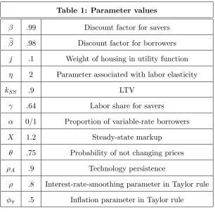
set to 1%, as in Iacoviello and Neri (2010). As in Rabanal (2004) and Iacoviello and Neri (2010), the degree of persistence of the demand shock is set to 0.80. Table 1 shows a summary of the parameter values.

Table 1: Parameter values

:99 Discount factor for savers e :98 Discount factor for borrowers

j :1 Weight of housing in utility function

2 Parameter associated with labor elasticity

kSS :9 LTV

:64 Labor share for savers

0=1 Proportion of variable-rate borrowers

X 1:2 Steady-state markup

:75 Probability of not changing prices

A :9 Technology persistence

:8 Interest-rate-smoothing parameter in Taylor rule

:5 In‡ation parameter in Taylor rule

2.5.2 Impulse Responses

To gain some insight into the dynamics of the model before studying macroprudential policies, Figure 1 presents impulse responses to a 1 % positive shock to technology with 0.9 degrees of persistence. We see that the economy responds slightly more strongly after a technology shock when the majority of its borrowers have a …xed-rate mortgage.

2 4 6 8 10 0 0.5 1 Output %d e v. ste a d y sta te

2 4 6 8 10

-5 0 5

Borrowing

2 4 6 8 10

0 1 2 Consumption Borrowers %d e v. ste a d y sta te

2 4 6 8 10

-0.2 0 0.2

Inflation

2 4 6 8 10

-5 0 5 Housing Borrowers quarters %d e v. ste a d y sta te

2 4 6 8 10

0 0.5 1 House Prices quarters Variable Fixed

Figure 1: Impulse responses to a technology shock.

consumption goods and this is why output ends up increasing by slightly more in the …xed-rate scenario. We can see from the dynamics of the model that having variable- or …xed-rate mortgages does not only a¤ect the macroeconomy but also the …nancial side. The …xed-rate economy has a less powerful monetary policy tool, but borrowers are more exposed to changes in in‡ation and house prices and thus this is going to a¤ect credit. Therefore, the structure of mortgage contracts has clear implications, not only for monetary policy reaction and for macro variables but also for house prices and borrowing. Thus, it seems clear that when including macroprudential policies, the mortgage contracts that are prevalent in the economy will a¤ect their implementation, because the macroprudential regulator cares about …nancial stability.

3

Modeling Macroprudential Policies

For the macroprudential policy, I will compare two options. The …rst one is a rule on the LTV, so that this variable responds to credit growth. The second one is an extended Taylor rule so that the interest rate, apart from responding to in‡ation and output, also responds to credit growth.

the interest rate, to achieve both macroeconomic and …nancial stability. In this case, the objectives of monetary policy should be expanded to include …nancial stability.

3.1 LTV Rule

As an approximation to a realistic macroprudential policy, I consider a simple rule for the LTV. In standard models, the LTV is a …xed parameter that is not a¤ected by economic conditions. However, we can think of regulations of LTVs as a way to moderate credit booms. When the LTV is high, the collateral constraint is less tight. Furthermore, because the constraint is binding, borrowers will borrow as much as they are allowed to. Lowering the LTV tightens the constraint and therefore restricts the loans that borrowers can obtain. Recent research on macroprudential policies has proposed simple rules for the LTV that inversely react to variables such as the growth rates of GDP, credit growth, the credit-to-GDP ratio or house prices. These rules are a simple illustration of how a macroprudential policy could work in practice. Here, we assume that there exists a macroprudential simple rule for the LTV, so that it responds to credit growth:36

kt=kSS(bt=bt 1) k

b _{; (31)}

where kSS is the steady-state value for the LTV. k_b 0 measures the response of the LTV to credit

growth. This type of rule would deliver a lower LTV in booms, when credit is growing, therefore restricting the credit in the economy and avoiding a credit boom caused by good economic conditions.

3.2 Macroprudential Taylor Rule

Here, I am considering the case in which the central bank adopts a macroprudential approach and monitors credit variables. Then, I extend the Taylor rule to not only respond to in‡ation and output growth but also to credit growth.

Rt= (Rt 1)

h _{(1+ )}

t (Yt=Yt 1) y(bt=bt 1) bR

i1

"Rt: (32)

3 6

Thus, we are giving the central bank a way to implement a macroprudential policy. Note that increasing the interest rate when credit is growing means restricting credit booms in the economy, because debt repayments are increasing. Therefore, in this case, the goals of the central bank are extended to also include …nancial stability.

4

Normative Analysis

In this section, I introduce the above mentioned macroprudential policies and study their implications for welfare and their optimal implementation. In order to do that, …rst I present a measure for welfare. Then, using this measure, I analyze the optimality of monetary and macroprudential policies for both …xed- and variable-rate mortgage economies and present impulse-responses using the optimized values.37 In new Keynesian models with collateral constraints, there are two types of distortions: sticky prices and credit frictions. Savers prefer policies that alleviate the …rst distortion, because they own the …rms. They are better o¤ in a scenario with price stability, the goal of monetary policy. However, borrowers’ welfare increases when the credit friction distortion is minimized. Then, borrowers may prefer situations that generate in‡ation, because in this case, the collateral constraint is relaxed through lower real debt repayments. On the one hand, monetary policy has e¤ects on the constraint directly through the interest rate that borrowers have to pay and indirectly through house prices, which makes collateral more or less valuable. On the other hand, macroprudential policies that deliver higher …nancial stability also lower the negative e¤ects of the credit friction, because they provide borrowers with a scenario in which their consumption is smoother.

However, these mechanisms di¤er depending on whether the prevalent mortgage contract in the economy is a …xed or variable rate. In the variable-rate scenario, monetary policy is more stabilizing because there is a direct link between the policy rate and the borrowing rate. Nevertheless, this link is broken for the …xed-rate case. Therefore, an economy with variable rates will be more e¤ective in minimizing the sticky price distortion, the one that a¤ects savers. In the …xed-rate scenario, borrowing is more dependent on in‡ation and house prices. Although the policy rate does not a¤ect the economy as much as in the variable-rate case, in‡ation a¤ects real rates and therefore borrowing. The policy rate also has an e¤ect on house prices, because as for any asset price, house prices move inversely with the interest rate, and thus also have an e¤ect on credit. Then, borrowers may prefer …xed rates

because it creates a situation with higher in‡ation and this lowers real debt repayments, thus relaxing their collateral constraint. Borrowers prefer situations in which the central bank is not able to …ght so e¤ectively against in‡ation, that is, in the …xed-rate case. In this case, even though in‡ation can rise or decrease, it would be in general higher than in a situation in which the central bank has a more powerful monetary policy tool, that is, in the variable-rate case. This is why, borrowers prefer …xed-rate scenarios. With respect to macroprudential policies, in the variable-rate case, the combination of monetary policy with an LTV rule would deliver more …nancial stability because, in a context of stable in‡ation, increasing LTVs in times of credit growth means containing credit. However, with …xed-rate mortgages, in which the real borrowing rate basically depends on in‡ation, higher in‡ation variability may o¤set the e¤ects of increasing the LTV, and greater …nancial stability may not be achieved.

When the macroprudential policy is included in the Taylor rule, for the variable-rate case, as other studies that include credit variables in the monetary policy rule show, there may be little gain in terms of welfare. However, for the …xed-rate case, it creates a new mechanism. Making the nominal rate respond to an additional variable that is more volatile than in‡ation and output makes house prices react by more than with the simple Taylor rule. This increases …nancial stability through the e¤ect of monetary policy on house prices.

4.1 Welfare Measure

As discussed in Benigno and Woodford (2008), the two approaches that have been used recently for welfare analysis in DSGE models include either characterizing the optimal Ramsey policy, or solving the model by using a second-order approximation to the structural equations for a given policy and then evaluating welfare using this solution. As in Mendicino and Pescatori (2007), I take this latter approach in order to be able to evaluate the welfare of the borrowers and savers separately and identify the trade-o¤ that appears between them.38

The individual welfare for savers and the two types of borrowers respectively are de…ned as follows:

Vu;t Et

1 X

m=0

m _lnCu

t+m+jlnHtu+m

Lu_t+m !

, (33)

Vcv;t Et

1 X

m=0

em _lnCcv

t+m+jlnHtcv+m

Lcv_t+m !

, (34)

3 8

Vcf;t Et

1 X

m=0

em

0

@lnC_tcf_+m+jlnH_tcf_+m

Lcf_t+m 1

A. (35)

Following Mendicino and Pescatori (2007), I de…ne social welfare as a weighted sum of individual welfare for the di¤erent types of households:

Vt= (1 )Vu;t+ 1 e [ Vcv;t+ (1 )Vcf;t]. (36)

Borrowers’and savers’welfare are weighted by 1 e and(1 ), respectively, so that the two groups receive the same level of utility from a constant consumption stream.

To make the results more intuitive, I present welfare changes in consumption equivalents, taking as a benchmark the situation in which there are no macroprudential policies.39

4.2 Optimal Policy

In this subsection, I study the mix of macroprudential and monetary policy that maximizes welfare. In particular, given a grid of possible parameters for the LTV and the Taylor rule (both the standard and the macroprudential ones), I perform a search that maximizes welfare, subject to the determinacy requirements.40 Parameters with a star correspond to the optimal ones, the ones that maximize welfare. I conduct the analysis …rst for the benchmark case, in which there are no macroprudential policies, so that I only optimize over the parameters of the standard Taylor rule. I …nd the parameters both for the variable- and the …xed-rate scenarios, as well as for an intermediate case in which the proportion of mortgages of each type is 50%. The results are presented in Table 2.

3 9

I follow Ascari and Ropele (2009).

Table 2: Optimized Taylor rule (benchmark) Variable rate =0:5 Fixed rate

(1 + ) 16 6:1 1:1

y 8:1 3:6 0

Volatilities

0:25 0:29 0:52

y 2:12 2:10 2:10

b 1:90 17:53 27:32

The results in Table 2 represent the benchmark case, because they do not include macroprudential policies. We can see the di¤erence in the optimality of monetary policy in both scenarios: …xed versus variable rates. For the variable-rate case, it is optimal for monetary policy to respond aggressively to both in‡ation and output. However, for …xed rates, because the link between the interest rate and the macroeconomic variables is weaker, it is not optimal for monetary policy to respond to any of the variables because in any case, the e¤ect of nominal rates on the economy is very limited; real rates matter more strongly in this case, and they are driven by in‡ation. Furthermore, the nominal interest rate, in this case, also a¤ects house prices and this also a¤ects borrowing. In terms of stability, we see from the volatilities that a degree of greater stability, both macroeconomic and …nancial, is achieved with variable-rate mortgages. Macroeconomic stability is achieved because monetary policy is more e¤ective with variable rates.41 With …xed rates, on the one hand, borrowers are more exposed to changes in house prices. On the other hand, because the nominal rate is …xed, the real rate depends mainly on in‡ation, and this one is more volatile than in the variable-rate case and real rates are more volatile. All this generates greater …nancial instability. The intermediate case lies in between the two extremes. We see that the optimal parameters do not imply a policy as aggressive as for the variable-rate case, but they are stronger than for the …xed one. In terms of in‡ation stability, the variable case is the one that delivers better results even though the variability of output is similar in all three cases.42 The variability

4 1_{See Rubio (2011) for a Taylor curve analysis that shows that monetary policy is more e¢ cient with variable-rate}

mortgages and therefore the economy is always more stable under this scenario.

4 2_{In models with borrowers and savers, it is usually the case that when one considers two di¤erent scenarios, for aggregate}

of borrowing in the mixed case also lies in between the two polar cases.

Table 3: Optimized Taylor and LTV rule Variable rate =0:5 Fixed rate

Taylor rule

(1 + ) 1:9 1:1 1:1

y 0:5 0:1 0

LTV rule

k

b 0:8 0:1 0:01

Welfare gain

Savers 0:40 0:99 0:98

Borrowers 0:68 1:43 5:09

Total 0:005 0:005 0:89

Volatilities

0:28 0:48 0:55

y 2:10 2:09 2:10

b 1:27 10:99 27:35

In Table 3, I present the optimized monetary policy when it interacts with an LTV rule. We see that, in this case, for the variable-rate scenario, the optimal response for monetary policy is substantially less aggressive than in the benchmark case without macroprudential policies in place. The macroprudential LTV rule complements the role of monetary policy,43 and both interacting together manage to achieve a more stable macroeconomic and …nancial scenario. However, this is at the expense of a slightly greater in‡ation volatility.44 _{The increase in in‡ation volatility makes savers worse o¤ because they care about}

the sticky-price friction. On the contrary, borrowers are better o¤ for two reasons; they like higher in‡ation because they have to repay their debt, and they prefer a more stable …nancial scenario, because this helps them smooth their consumption.45

4 3_{The sense in which macroprudential policy is complementary to monetary policy is that a similar level of in‡ation}

volatility is achieved with considerably less aggressive monetary policy. In addition, the volatility of debt is substantially reduced.

4 4_{This is a typical result found in the literature. The results are in line, for example, with Gelain et al. (2013) who}

show that while macroprudential policies can stabilize some variables, they can magnify the volatility of others, especially in‡ation.

4 5

For the intermediate and the …xed-rate case, the optimal reaction of both monetary and macropru-dential policies is smaller then that in the variable-rate scenario. Monetary policy is still not e¤ective, and therefore the optimal response is minimal, as in the benchmark case. The introduction of the LTV rule has similar e¤ects to those in the variable-rate scenario. It does not worsen the volatility of output but it increases the volatility of in‡ation. As remarked by Lustig (2006) and Rubio (2011), the in‡ation channel that relaxes borrowing constraints should be much more e¤ective when …xed-rate mortgages are predominant, because agents care about real rates. Therefore, agents are more sensitive to changes in in‡ation in a …xed-rate scenario. This is the reason why borrowers’ welfare gains and savers’ losses are larger in this case, even though in the aggregate, losses outweigh gains. However, in the …xed-rate case, welfare gains come mainly from the fact that in‡ation is more volatile, but not from the …nancial side. Given that in‡ation is less stable, borrowers bene…t in terms of debt repayments, relaxing their constraint. This o¤sets the constraint tightening that the LTV rule should impose. As a result, although the economy is better o¤, greater …nancial stability is not achieved. In the intermediate case, there is some gain in terms of …nancial stability though.

Table 4: Optimized macroprudential Taylor rule Variable rate =0:5 Fixed rate

(1 + ) 13:1 1:1 1:1

y 6 0:1 0

b 0:9 0:1 0:01

Welfare gain

Savers 0:09 0:99 0:99

Borrowers 0:09 1:94 4:47

Total 0:007 0:30 1:77

Volatilities

0:24 0:63 0:54

y 2:12 2:11 2:11

b 1:93 19:73 20:57

In Table 4, the macroprudential policy is introduced directly in the Taylor rule, by letting the interest rate respond to credit growth. The results show that, although it is optimal to respond to credit growth,

the optimal monetary policy is aggressive, as in the case in which the central bank only responds to in‡ation and output. As is common in the literature, for the standard variable-rate case, there are no welfare gains from responding to credit variables.46 Table 4 shows that in‡ation volatility is slightly lower than in the benchmark case and …nancial instability slightly larger. Thus, with this new optimized Taylor rule, borrowers are slightly worse o¤ with respect to the case in which credit variables are not included in the rule because in‡ation is less volatile, although there are no bene…ts from the …nancial side. This is o¤set by the fact that savers live in a slightly more stable world.

However, for the intermediate and the …xed-rate cases, the gains are larger, coming mainly from the borrowers’ side. When the nominal rate responds to credit growth, it reacts more strongly to changes in the economy. Even though the optimal response is small, credit is a volatile variable and thus the interest rate responds more strongly than with the standard Taylor rule. This has an e¤ect on house prices and the collateral constraint is a¤ected through this channel. For example, if there is an increase in credit, the interest rate will increase and this will decrease house prices. The fall in house prices tightens the collateral constraint and helps achieve greater …nancial stability. A scenario with greater …nancial stability is bene…cial for borrowers. This is an example of a theory of second best, given the distortion that the collateral constraint is introducing.

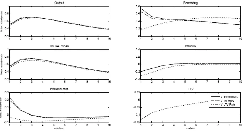
4.3 Impulse Responses

Figure 2 presents the impulse responses to a technology shock for a variable-rate economy and for the optimized parameters found in Tables 2-4.47 The technology shock increases output and decreases in‡ation. As a result, the interest rate increases slightly, to respond to the increase in output, especially in the case in which the interest rate responds to credit growth. For the case in which the macroprudential policy is represented by an LTV rule, the interest rate decreases because the optimal reaction parameters in the Taylor rule are much smaller than in the other two cases. It also re‡ects that relatively more weight is placed on in‡ation relative to output in this instance. The borrowing interest rate in this case varies one-for-one with the policy rate. House prices move as a mirror image of the interest rate and also respond to the increase in housing demand derived from better economic conditions. As house prices increase, borrowing increases. However, the increase in borrowing is softer in the case in which

4 6_{See, for instance, Iacoviello (2005), who shows with a policy frontier analysis that little is gained in terms of in‡ation}

and output stabilization by responding to asset prices. Christiano et al. (2014) also …nd that consumption falls after a rise in risk.

4 7

Figure 2: Impulse responses to a technology shock: variable rate.

macroprudential policies are present. When the macroprudential policy is incorporated in the Taylor rule, the increase in the interest rate is larger and then, borrowing increases by less on impact, although the e¤ect dissipates in subsequent periods. However, borrowing is really contained when the LTV rule is active. In this case, as a reaction to credit growth, the macroprudential regulator cuts the LTV, making credit less accessible for borrowers. For this latter case, the macroprudential measure mitigates the e¤ect of the technology shock.

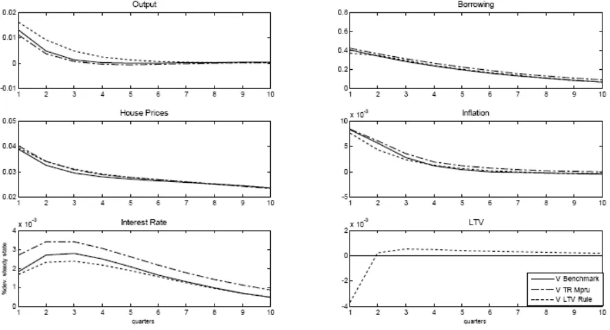
Figure 3: Impulse responses to a technology shock: …xed rate.

this case, borrowers devote less income to purchasing houses and purchase more consumption goods, making output increase by more in this scenario. The decrease in credit makes the LTV increase, when the LTV rule is active and, on impact, credit does not decrease as much, although the e¤ect diminishes very quickly. Thus, while real rates decrease in the variable-rate scenario, they increase in the …xed-rate one, making borrowing and LTVs (for the LTV rule case) move in opposite directions.

much di¤erence in this case with respect to the benchmark.

5

Conclusions

In this paper, I studied the ability of monetary policy to a¤ect …nancial markets under both …xed- and variable-rate mortgages. I have developed a new Keynesian general equilibrium model with housing and collateral constraints to analyze the combined e¤ects of macroprudential and monetary policies with these two types of mortgage contracts. There are unconstrained and constrained individuals who correspond to the savers and borrowers of the economy. I explicitly introduced …xed- and variable-rate mortgages, that is, constrained individuals are of two types: those who borrow at a variable rate and those who borrow at a …xed rate.

First, in order to gain some insight, I studied the dynamics of the model for the case in which there are no macroprudential policies. The results show that having variable- or …xed-rate mortgages not only a¤ects the macroeconomy but also the …nancial side of the economy. Therefore, the structure of mortgage contracts has clear implications, not only for monetary policy reaction and for macro variables, but also for the implementation of macroprudential policies.

I proposed two types of macroprudential policies. The …rst one is a simple rule on the LTV. In this case, the LTV would be the instrument of the macroprudential regulator, responding to credit growth. The second one is a Taylor rule for the interest rate, in which rates would respond not only to in‡ation and output but also to credit growth. In this second case, both monetary and macroprudential policies would be implemented with a single instrument; the interest rate.

environment. For the …xed-rate case, the optimal reaction of both monetary and macroprudential policies is smaller than that in the variable-rate scenario. Welfare gains, however, come mainly from the fact that in‡ation is more volatile but not from the …nancial side. Finally, I studied the welfare and optimality implications of including credit growth directly in the Taylor rule for the interest rate. For the standard variable-rate case, the welfare gains of responding to credit variables are very small. Albeit, for the …xed-rate case gains are larger, coming mainly from the borrowers’ side because this delivers greater …nancial stability.

References

[1] Alpanda, S., Zubairy, S., (2014), Addressing Household Indebtedness: Monetary, Fiscal or Macro-prudential Policy?, Sta¤ Working Papers 14-58, Bank of Canada

[2] Andrés, J., Arce, O., Thomas, C., (2009), Banking Competition, Collateral Constraints and Optimal Monetary Policy, mimeo

[3] Angelini, P., Neri, S., Panetta, F., (2014), "The Interaction between Capital Requirements and Monetary Policy," Journal of Money, Credit and Banking, Volume 46, Issue 6, pp. 1073–1112

[4] Aoki, K., Proudman, J., Vlieghe, G., (2004), "House Prices, Consumption, and Monetary Policy: A Financial Accelerator Approach," Journal of Financial Intermediation, 13 (4), 414-435

[5] Assenmacher-Wesche K., Gerlach, S., (2008), Ensuring Financial Stability: Financial Structure and the Impact of Monetary Policy on Asset Prices, Institute for Empirical Research in Economics, University of Zurich, Working Paper 361

[6] Basel Committee on Banking Supervision, (2010), “Guidance for national authorities operating the countercyclical capital bu¤er,” Bank for International Settlement publication

[7] Benigno, P., Woodford, M., (2008), Linear-Quadratic Approximation of Optimal Policy Problems, mimeo

[8] Brzoza-Brzezina, M., Gelain, P., Kolasa, M., (2014), Monetary and macroprudential policy with multiperiod loans, NBP Working Paper No. 192

[9] Calza, A., Monacelli, T., Stracca, L., (2013), "Housing Finance and Monetary Policy," Journal of the European Economic Association

[10] Calvo, G., (1983), "Staggered Prices in a Utility-Maximizing Framework," Journal of Monetary Economics, 12 (3), 383-398

[11] Campbell J., Cocco, J., (2003), "Household Risk Management and Optimal Mortgage Choice," Quarterly Journal of Economics, 118 (4), 1449-1494

[12] Christiano, L., Motto, R., Rostagno, M., (2014), "Risk Shocks," American Economic Review, 104 (1), 27-45

[13] Clarida, Galí, Gertler, (2000), "Monetary Policy Rules and Macroeconomic Stability: Evidence and Some Theory," Quarterly Journal of Economics, 115, 147-180

[14] Davis, M., Heathcote, J., (2005), "Housing and the Business Cycle," International Economic Review, 46 (3), 751-784

[15] Debelle, G., (2004), "Household Debt and the Macroeconomy," BIS Quarterly Review

[17] EMF, (2006), "Study on Interest Rate Variability in Europe," EMF Publication

[18] Faia, E., Monacelli, T., (2007), "Optimal Interest Rate Rules, Asset Prices, and Credit Frictions," Journal of Economic Dynamics and Control, 31, 3228-3254

[19] Fuhrer, J., Moore, G., (1995), "In‡ation Persistence," Quarterly Journal of Economics, February 1995, 110 (1), pp. 303-36.

[20] Garriga, C., Kydland, F., Sustek, R., (2015). "Mortgages and Monetary Policy," Working Papers 2015-33, Federal Reserve Bank of St. Louis.

[21] Gelain, P., Lansing, K., Mendicino, C., (2013), "House Prices, Credit Growth, and Excess Volatility: Implications for Monetary and Macroprudential Policy," International Journal of Central Banking, 9 (2)

[22] Graham, L., Wright, S., (2007), "Nominal Debt Dynamics, Credit Constraints and Monetary Pol-icy," The B.E. Journal of Macroeconomics, 7 (1)

[23] Iacoviello, M., (2005), "House Prices, Borrowing Constraints and Monetary Policy in the Business Cycle," American Economic Review, 95 (3), 739-764

[24] Iacoviello, M., Neri, S., (2008), Housing Market Spillovers: Evidence from an Estimated DSGE Model, mimeo

[25] Kannan, P., Rabanal, P., Scott, A., (2012), "Monetary and Macroprudential Policy Rules in a Model with House Price Booms," The B.E. Journal of Macroeconomics, Contributions, 12 (1)

[26] Krusell, P., Smith, A., (1998), "Income and Wealth Heterogeneity in the Macroeconomy," The Journal of Political Economy, 106 (5), 867-896

[27] Lawrance, E., (1991), "Poverty and the Rate of Time Preference: Evidence from Panel Data," The Journal of Political Economy, 99 (1), 54-77

[28] Lustig, H., (2006), Comment on "Optimal Monetary Policy with Collateralized Household Debt and Borrowing Constraints," in conference proceedings "Monetary Policy and Asset Prices" edited by J. Campbell.

[29] Mendicino, C., Pescatori, A., (2007), Credit Frictions, Housing Prices and Optimal Monetary Policy Rules, mimeo

[30] McCallum, B., (2001), "Should Monetary Policy Respond Strongly To Output Gaps?," American Economic Review, 2001, 91(2), 258-262

[31] Monacelli, T., (2006), "Optimal Monetary Policy with Collateralized Household Debt and Borrowing Constraints," in conference proceedings "Monetary Policy and Asset Prices" edited by J. Campbell.

[33] Rubio, M., (2011), "Fixed- and Variable-Rate Mortgages, Business Cycles, and Monetary Policy," Journal of Money, Credit and Banking, 43 (4), 657-688

[34] Rubio, M., Carrasco-Gallego, J.A., (2014), "Macroprudential and Monetary Policies: Implications for Financial Stability and Welfare," Journal of Banking and Finance

[35] Rubio, M., Carrasco-Gallego, J.A., (2015), "Macroprudential and Monetary Policy Rules: A Welfare Analysis," The Manchester School

[36] Shea, P., (2008), Interest Rate Rules, Learning, and Credit Constrained Housing Markets, mimeo

[37] Smets, F., Wouters F., (2002), An Estimated Stochastic General Economic Model of the Euro Area, ECB WP 171

Appendix

Tables and Figures

Table A1: Predominant Type of Mortgage Interest Rate Australia Variable Italy Mixed

Austria Fixed Japan Mixed

France Fixed Spain Variable

Germany Fixed United Kingdom Variable

Greece Variable United States Fixed Source: ECB (2003), IMF

Table A2: Sensitivity Analysis to di¤erent values of Variable rate Fixed rate

0:95 0:96 0:97 0:98 0:95 0:96 0:97 0:98

Volatilities

0:27 0:27 0:26 0:26 0:22 0:21 0:21 0:20

y 2:25 2:25 2:24 2:24 2:37 2:36 2:35 2:33

b 5:41 5:55 5:71 5:87 11:75 12:04 12:34 12:63

Table A3: Sensitivity Analysis to di¤erent values of Variable rate Fixed rate

0:2 0:5 0:64 0:9 0:2 0:5 0:64 0:9

Volatilities

0:27 0:21 0:26 0:33 0:35 0:18 0:20 0:29

y 2:56 2:29 2:24 2:19 2:41 2:33 2:33 2:26

Figure A1: Impulse Responses to an Expansionary Monetary Policy Shock. Variable Rates.

Figure A3: Impulse Responses to a House Price Shock. Variable Rates.

Figure A5: Impulse Responses to a Demand Shock. Variable Rates.

Model Derivations

Steady-State Relationships

Using(9) in the steady state we obtainR = 1= . From (5)and (6) we have thatR =R=R= 1= . From the …rst order conditions for housing we can obtain the steady-state consumption-to-housing ratio for both constrained and unconstrained consumers:

Cu

qHu =

1

j(1 ); (37)

Cc

qHc =

1

j 1 e kSS e =

1

j ; (38)

where 1 e kSS e . From(19)and(27)we obtain the constrained and unconstrained

consumption-to-output ratio in the steady state:

Cc

Y =

1

X +jkSS(1 )

; (39)

Cu

Y = 1

Cc

Y ; (40)

where X="=(" 1)

The housing-to-output ratio for constrained and unconstrained consumers:

qHc

Y =

(1 )j X

1

+jkSS(1 )

; (41)

qHu

Y =

Xj( +jkSS(1 )) j(1 )

X( +jkSS(1 )) (1 )

: (42)

Log-Linearized Model