Economic evaluation of installation of standalone wind farm and Wind+CAES system for the new regulating tariffs for renewables in Egypt

Economic Evaluation of installation of standalone wind

farm and Wind+CAES system for the new regulating

tariffs for renewables in Egypt

Omar Ramadan

, Siddig Omer, Yate Ding, Hasila Jarimi, Xiangjie Chen, Saffa Riffat

Department of Architecture and Built Environment , Faculty of Engineering, University of Nottingham, University Park, Nottingham, NG7 2RD

E-mail address: [email protected]

Abstract

Compressed Air Energy Storage (CAES) is widely recognized as a viable solution for large-scale grid integrated renewable energy systems in terms of load levelling to solve/minimize the intermittency effect of renewable energy systems especially with increased penetration of renewables to the grid. This study assesses the economic value of adding compressed air energy storage (CAES) plant to a renewable energy system and how this impacts the overall financial appeal of the system at hand, taking Egyptian grid as a case in point. Numerical modelling using MATLAB was performed to analyse the benefits of adding a CAES system to planned wind farms in Egypt by 2020 for both load-levelling as well as optimizing economic benefit. The results show that the addition of a CAES system would increase the profitability for the new Tariff for wind systems set by the Egyptian government with a NPV of $306m compared to a NPV of $207m of a stand-alone wind system at the end of 25 years of operation. Also, the economic benefits increase if the government provides subsidies for new installations of renewable energy systems, or by lowering the interest rates.

Keywords:

Compressed Air Energy Storage (CAES), Economic Assessment, Energy Storage systems, Wind Energy, Large scale renewable energy

Nomenclature

ACw Annual costs of the wind farm [$]𝐴𝑇_{𝐶𝐴𝐸𝑆2} annual O&M costs of CAES [$]

𝑐_𝑐 specific compressor cost ($/MW) ct specific turbine cost ($/MW)

Cw capital cost for wind farm[$]

ηc polytropic efficiency of the compressors

ICCAES Initial capital cost of CAES [$]

mt mass flow rate during expansion [kg/s]

mc mass flow rate during compression [kg/s]

Pmax maximum allowable pressure in cavern [bar]

Pcav pressureof air in the cavern [bar]

P1 pressure at compressor inlet [bar]

P2 pressure of air at the compressor outlet [bar]

P3 pressure at turbine inlet [bar]

P4 pressure of air at the turbine outlet [bar]

Pw energy supplied from the wind [KWh]

Pm market price for wind energy [cent$/KWh]

𝑃𝑡 turbine rated power[MW] 𝑃_𝑐 compressor rated power[MW] 𝜌 compressed air density [kg/m3] R universal gas constant

ROI return on investment 𝑅_{𝐶𝐴𝐸𝑆} annual CAES revenues [$]

T1 temperature at compressor inlet [K]

T2 temperature of air at the compressor outlet [K]

Tcav temperature of air in the cavern [K]

T3 temperature at turbine inlet [K]

T4 temperature of air at the turbine outlet [K]

Vcav volume of underground cavern [m3]

1.

Introduction

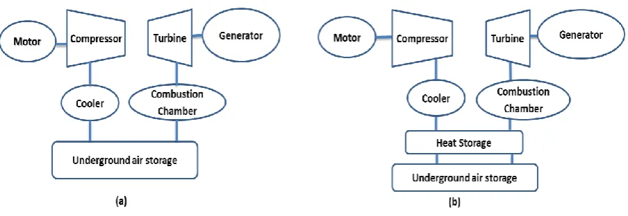
re-heat the air during the generation (expansion) cycle. In an adiabatic compressed air energy storage system, the heat generated from the compression stage is stored using thermal energy storage, rather than being vented. The stored thermal energy is then used later to heat the air which is passing from the underground cavern into the expander turbine, to reduce/eliminate the use of fuel in expansion stage, with the result being lower cost, higher efficiency and less harmful emissions and less environmental impact.

Figure 1 CAES system (a) diabetic and (b) adiabatic

1.1 Recent Research carried out on CAES system economic value

1.2 Egyptian electricity market case

Up until early 1990s, Egyptian ministry of electricity was in full control of all power generation, transmission and distribution activities. In 1996, the government issued a law allowing local and foreign investors to build, own, operate and later transfer (BOOT) generation stations to the state; this has led to the establishment of 4 private companies, selling mostly to the government as governed by long-term contracts dictating dollar-denominated pre-set prices, and based on subsidized natural gas supplied to those companies by the government. In 2001, the private sector was further allowed to supply power to particular consumers, like factories, at which time a handful of private electricity generation companies started up, and a number of factories established their own power plants as an emergency backup. However, they could only sell electricity at modest prices set by the state, which was again feasible at that time with subsidized gas prices. This, however saw the government’s Electricity Holding Company (mother company responsible for some 16 other state-owned enterprises) accumulate losses of EGP163m as of July, cost the government fifth of its public spending in subsidies, and shut out all private investors. Hence, to attract investments, it was necessary to liberate generation and distribution from the state’s grip, and to hand these activities over to private companies with sustainable and profitable business models, creating a free market that is more viable for all parties. Therefore, in 2015, the government issued the New Electricity Law that dictates the grid feed-in-tariff for renewable energy independent power producers (IPPs), with the tariff for electricity generated from conventional fuels set to follow shortly. It also completed the unbundling of generation, transmission, and distribution to unwind the single-buyer mechanism and pave the way for competition and free market operation, supported by direct bilateral agreements and third-party access to transmission and distribution networks. This was especially inevitable following the government’s enforcement of a plan to phase out energy subsidies over the next 5 years, in another move to free the markets, lure investments and push for much-needed fiscal consolidation. As power suppliers compete for customers, service should improve, prices should stay low, pressure on the national grid be relieved, and more room be allowed for the Holding company to overhaul some 20-year old generation and distribution networks making up 40% of capacity. While the regulator would still intervene to prevent unreasonable price hikes and monopolies, the long-term target is to create a real open market for electricity, much like any other freely traded product [15, 16].

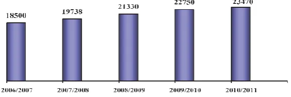
Figure 2Annual peak load demand in Egypt (MW)

Figure 3 [16] shows the variation of the load demand pattern for a summer day in Egypt. The variation of load demand in winter has a similar pattern with a lower peak load.

Figure 3Variation of the load demand in Egypt in the month of June in 2009

There are large unexploited resources for renewable energy in Egypt, yet the application of renewable energy technologies in Egypt has been rather limited. However, there are future plans to increase the renewable energy supply greatly in the next decade to supply 20% of the total energy capacity, 12% of which is projected to be provided by wind energy. This assumes an increase of the installed wind energy capacity to 7.2 GW from 780 MW by 2020 [17]. Wind energy resource is to a certain extent widely available in Egypt and is particularly high in the Suez area. Figure 4 presents the wind map for Egypt, showing the areas with highest wind speeds.

1 3 6 9 12 15 18 21

0 5 10 15 20 25

time(hours)

Pow

er

(GW

)

Figure 4 Wind Map of Egypt

2.

Methodology and Results

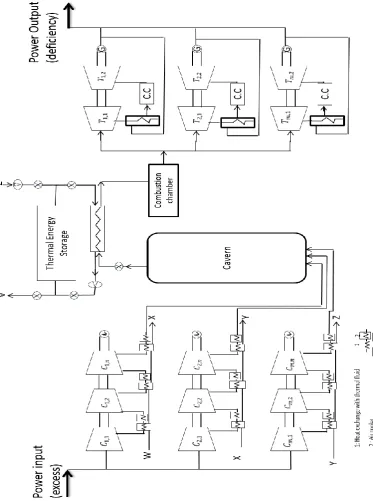
The operation of a CAES plant uses compressor to compress air when the supply is higher than demand, the compressed air is stored in large underground cavern (reservoir), when the load demand is higher than the power supply, the compressed air powers turbines to generate power is shown in Figure 1. Thermal energy storage could be used in adiabatic system to reduce the use of natural gas and improve the performance of the system. MATLAB programing is used to simulate a model for both sizing a CAES system to accommodate the difference between the supply and the demand and also the economic performance of the modelled CAES system. Firstly, the compressors and the turbines are sized based on the maximum surplus power available during the compression and maximum deficiency in power during expansion modes respectively. The cavern is then sized depending on the mass flow rates of air as well as number of hours of operation for each mode.

2.1 Sizing and performance of a CAES system for load-levelling

The technical sizing and performance of the CAES system is modelled using dynamic computer modelling to show the technical benefits of implementing a CAES system to solve the intermittency issues of renewable energy systems taking the Suez area in Egypt as a case study.

2.1.1 Simulation Assumptions

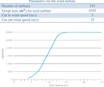
The system is based on the planned projects in Suez, which currently has an installed wind capacity of 580 MW [17]. This is modelled as a sole wind farm using 193 (V90-3MW) Vestas wind turbines, 3MW each. Vestas wind turbines are selected due to the compatibility of these wind turbine characteristics with the weather data at the case study location. Table 1 shows the operating parameters of the selected wind turbines. The power curve for the VESTAS wind turbines in this simulation is presented in Figure 5 [18]. The collected data for the wind speeds in the Suez area is for three consecutive summer days is shown in Figure 6. The sizing of the CAES system components are implemented using the wind speed data.

Table 1 Suez project assumed parameters

Parameters for the wind turbine

Number of turbines 193

Swept area (𝒎𝟐) for each turbine 6362

Cut in wind speed (m/s) 3

Cut out wind speed (m/s) 25

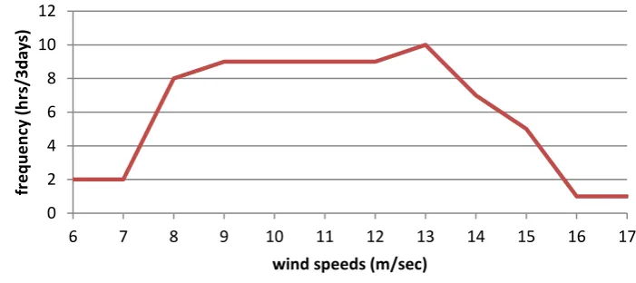
Figure 6 Frequency of wind speeds for 3 summer days at Suez area

Based on the wind speed data obtained, it is concluded that the wind energy potential at the case study location varies between 6 m/s to 17 m/s based on weather data monitoring during summer days [19], and these matches well with the Vestas wind turbine operating conditions.

2.1.2 Design Sizing

First, the CAES system is sized to meet the load demand conditions of Suez project. Following the sizing of the system components, dynamic modelling is used to forecast the operational behaviour of the CAES system. Figure 7 shows the excess and the deficiency in power which are the result of the difference between the forecasted power supply and the load demand in the location of the case study by 2020, which is displayed by the green curve. Hence, according to Figure 7, the compression stage starts when the excess/deficiency in power is positive. This should last for 17 hours during the first compression process. When the excess/deficiency in power is negative, the expansion starts, for around 13 hours for the first expansion stage. The charging and discharging periods are essentially diversifying due to the variation of the power supply and load demand.

Figure 7 Hourly variation of the load, wind power and excess/deficiency power

a) Compressors Sizing

The compressors are divided into a number of series and parallel chains. The parallel chains number is determined by the desired lowest output following the parallel chains method [19]. In this case, 4 parallel

0 2 4 6 8 10 12

6 7 8 9 10 11 12 13 14 15 16 17

fr e q u e n cy (h rs/3d ay s)

wind speeds (m/sec)

0 6 12 18 24 30 36 42 48 54 60 66 72

-400 -200 0 200 400 600 800 Time (hours) Po w er (M W )

Forecasted load demand in Suez, Egypt by 2020 Excess/ Difficiency in power

chains of compressors were selected to cater for lower powers by operating compressors close to their rated power, or 1/15 of the maximum power available for the compressors. For the CAES system sizing with MATLAB, it was concluded that the maximum compressor power (peak difference between wind power output and load demand) required for the highest surplus power is 277.5 MW. Since parallel chains are used for the CAES system, hence the minimum power that the implemented CAES design can supply, is given by the following:

𝐿𝑜𝑤𝑒𝑠𝑡 𝑟𝑎𝑡𝑒𝑑 𝑐ℎ𝑎𝑖𝑛 =𝑃𝑠𝑢𝑟𝑝𝑙𝑢𝑠𝑚𝑎𝑥

(8+4+2+1) = 18.5𝑀𝑊 (1)

Second chain comprise of 2/15 of the maximum power followed by the 3rd _{chain comprising 4/15 of the}

maximum power and then 4th chain of rated power of 8/15 of maximum power available. Figure 8 shows the compressors design with the number of chains and the maximum power for each. There are 4 parallel chains with the lowest rated at 18.5MW and the highest rated at 148MW, there is a heat exchanger between each compressor and the following compressor for intercooling followed by an air cooler for each stage. The heat transfer fluid on the other hand flows in a series fashion.

Figure 8 Sketch illustrating the CAES system configuration

b) Cavern Sizing

The volume of the CAES cavern sizing is performed using a method which ensures that the cavern is big enough to allow the system to be in operation during the compression or expansion periods. This means that for the sizing method used, the cavern should never be empty. The volume of the cavern is designed, based on the mass flow rate of air incoming or leaving the cavern. It also uses the number of consecutive hours in which the system is in compression mode or expansion mode, which is calculated using the historical data of the excess/ deficiency results from wind supply and load demand data. For the volume of cavern to satisfy these conditions, it is calculated to be 1,110,000 𝑚3 _using

𝑉𝑐𝑎𝑣= max ((𝑚𝑡× 𝑇𝑖𝑚𝑒𝑒𝑥𝑝𝑎𝑛𝑠𝑖𝑜𝑛) , (𝑚𝑐× 𝑇𝑖𝑚𝑒𝑐𝑜𝑚𝑝𝑟𝑒𝑠𝑠𝑖𝑜𝑛)) × _𝑃𝑅×𝑇𝑚𝑎𝑥

Where,

𝑉𝑐𝑎𝑣 is the volume of the cavern (𝑚3);

𝑚_𝑡 𝑎𝑛𝑑 𝑚_𝑐 are the mass flow rate from the compressors to the cavern and the mass flow rate from the cavern to the turbines respectively (𝑘𝑔/𝑠);

𝑇𝑖𝑚𝑒𝑒𝑥𝑝𝑎𝑛𝑠𝑖𝑜𝑛and 𝑇𝑖𝑚𝑒𝑐𝑜𝑚𝑝𝑟𝑒𝑠𝑠𝑖𝑜𝑛are the number of consecutive hours of expansion and compression time

respectively

𝑅 is the universal gas constant (𝐽/𝑚𝑜𝑙. 𝐾);

𝑇_𝑚𝑎𝑥 is the maximum operating temperature of air in the cavern (K);

𝑃𝑚𝑎𝑥and 𝑃𝑚𝑖𝑛 are the maximum and minimum limits of the pressure of air in the cavern, determined by the geology of the location and specifications of the turbines (pascals).

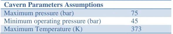
The maximum and minimum allowable pressure in the cavern depends on the geology of the location (Suez Area) and are estimated at 75 bar and 45 bar respectively, with a maximum operating temperature of air in the cavern assumed at 373K. The heat exchangers will be operating at different capacity rates, and their effectiveness are likely to vary accordingly, but for simplicity the heat exchangers effectiveness is assumed at 85%; while the temperature of the wall of the cavern is assumed to be 303K.

Table 2. Cavern operation parameters

Cavern Parameters Assumptions

Maximum pressure (bar) 75

Minimum operating pressure (bar) 45

Maximum Temperature (K) 373

c) Turbine Sizing

Using the same procedure in the sizing of the compressor, the sizing of the turbines is performed, resulting in a maximum power output needed from the turbines of around 300MW, leading to 4 parallel chains. The whole set of turbines are configured as shown in Figure 8 with combustion chambers between each series of turbines.

2.1.3 Operational modelling of the CAES system

a) Compressors operation

When there is excess wind power supply, the surplus power is used to power the compressors. The equations governing each compression stage are given by [20]:

(𝑃2

𝑃1)

(𝛾−1_𝛾 ) =𝑇2

𝑇1 (3)

𝛾 is the specific heat ratio

𝑃₂𝑎𝑛𝑑 𝑇₂ are the pressure and temperature of air at the compressor outlet, respectively .

b) Operation of the underground air storage cavern

In the cavern, the internal energy of the air in the cavern increases when the compressed air enters the cavern, and conversly when the air leaves the cavern during the expansion stage. The rate of change of the internal energy in the cavern is given by [21]:

𝑑 (𝑀𝑡𝑜𝑡𝑎𝑙(𝑡)𝑈

𝑑𝑡 ) = 𝑚̇𝑐𝐻𝑐− 𝑚̇𝑇𝐻𝑇− ℎ𝐴𝑐𝑎𝑣(𝑇𝑐𝑎𝑣− 𝑇𝑠𝑢𝑟𝑟𝑜𝑢𝑛𝑑𝑖𝑛𝑔) (4) Terms 1 and 2 on the right hand side are the variation in enthalpy which results from the flow of air in and out of the cavern. 𝑀_{𝑡𝑜𝑡𝑎𝑙}(𝑡) represents the instantaneous total mass of air in the cavern at a given time, which also changes with the incoming compressed air flow rate from the compressor or outgoing air flow to the turbine. 𝐻_𝑐is the specific enthalpy of the incoming air from the compressors, where 𝐻_𝑇 is the specific enthalpy of the outgoing air. The last term on the left represents the thermal losses from the cavern air to the surroundings, where ℎ is the heat transfer coefficient between the cavern wall and the air and 𝐴𝑐𝑎𝑣 is the area of heat transfer between the reservoir wall and the stored air.

For an ideal gas:

𝑢 = 𝐻 −

𝜌 (5)

Substituting Equation (5) in Equation (4) will result in: 𝜌𝐶𝑝𝑑𝑇_𝑑𝑡 +𝑚̇𝑐𝐶𝑝(𝑇𝑐𝑎𝑣−𝑇𝑖𝑛𝑙𝑒𝑡

)

𝑉𝑐𝑎𝑣 −

𝑑𝑃

𝑑𝑡+ ℎ𝑐(𝑇𝑐𝑎𝑣− 𝑇𝑤𝑎𝑙𝑙) = 0 (6) ℎ_𝑐 is the effective heat transfer coefficient and it is a function of air flow rates in and out of the cavern. 𝑑𝑃

𝑑𝑡 represents the variation of pressure with time during system operation. 𝜌 is the compressed air density. 𝑇_{𝑖𝑛𝑙𝑒𝑡} is the temperature of the incoming air from the compression stage.

𝑀_{𝑡𝑜𝑡𝑎𝑙} changes according to the rate of air inflow into the cavern. 𝑇_𝑐𝑎𝑣 also changes during the course of the system operation, and denotes average cavern temperature. Hence, the pressure variation in the cavern during the operation of the CAES system is calculated using the instantaneous values of the temperature and mass of air in the cavern. Assuming a molar weight of air of 0.029 𝑘𝑔:

𝑃_𝑐𝑎𝑣 = (𝑀𝑡𝑜𝑡𝑎𝑙×𝑅×𝑇𝑐𝑎𝑣

0.029×𝑉𝑐𝑎𝑣 ) (7)

𝑀_{𝑡𝑜𝑡𝑎𝑙} is the mass of the air in the cavern 𝑅 is the universal gas constant

c) Operation of the turbines (power generation stage)

The turbine output is dependent on the enthalpy flow of the air stream through the turbine and is given by:

𝐻̇ = 𝑚̇𝑇𝐶𝑝_𝑎𝑖𝑟𝑇𝑎𝑖𝑟 (8) where 𝐶_{𝑝_𝑎𝑖𝑟} is the specific heat of air and is assumed to be constant at 1005 𝐽 𝑘𝑔. 𝐾.⁄

The outlet temperature of the expansion process is given by: (𝑃4

𝑃3)

((𝑛−1)_𝑛 )

= 𝑇4

𝑇3 (9)

𝑛 is the polytropic index for the expansion stage

𝑃3 𝑎𝑛𝑑 𝑇3 are the pressure and temperature before the expansion in the turbine, respectively 𝑃₄ 𝑎𝑛𝑑 𝑇₄ are the pressure and temperature after the expansion in the turbine, respectively

2.2 Operational Results of the CAES system

A MATLAB program is developed to predict the operational performance of the CAES system. In this section, the results for the CAES system parameters are discussed using an adiabatic system with an added thermal energy storage. Figure 9 shows the pressure and temperature variation of the air in the cavern during the 3 days of operation. The variation of the pressure and temperature are calculated and plotted against the operation time. When there is a surplus of power, the pressure inside the cavern increases to around 68 bar after 17 hours of operation, and then the expansion mode starts. The pressure never reaches the minimum allowable value of 45 bar, which indicates that there is sufficient compressed air to meet the demand in the discharging period. The temperature increases in the compression stages and decreases in the expansion processes as expected. The rate of change of temperature is changing with time, which is dependent on the mass flow rate in and out of the cavern.

Figure 9 Hourly variation of the cavern air pressure (bar)/temperature (°C) 0 10 20 30 40 50 60 70 80 0 10 20 30 40 50 60 70 80 90 100

0 6 12 18 24 30 36 42 48 54 60 66

Figure 10 shows the variation of surplus energy stored and used as a result of implementing a CAES system. The power supplied to the CAES system (charging mode) when there is excess in power supply, is displayed by the blue area in figure 10. On the other hand, when the load demand is higher than the supply, the power is provided by the CAES system to the grid (grey area). The CAES system is able to provide enough power needed to cover the deficiency in power supplied by wind. This figure shows the value a CAES system could add to a grid system to decrease the effect of renewable energy intermittency and hence encourage high levels of penetration of renewable energy systems to the grid.

Figure 10 CAES operation mode for load levelling

3.

Economic evaluation of the CAES system

3.1 Methodology of economic modelling of the wind plant installation

In this section, the economic added value is discussed in more detail; however the operation mode of CAES differs for profit maximization approach which depends on the tariffs dictated by the laws of the location of the case study. The steps of simulation include the calculation of the system’s total annual revenues. Capital costs are also calculated, converted into yearly payments, and added to the system’s total fixed and variable annual costs. The annual net profit/loss and the return on investment (ROI) are calculated accordingly, and used as a measure of economic feasibility. Two systems are simulated, the first being the implementation of a wind farm with no CAES system, and the second simulating the integration of a CAES system to the wind farm. The analysis is performed using MATLAB program in section 3.3.

For each scenario, the system’s annual net present value (NPV) and annual ROI are calculated. Additionally, a sensitivity analysis is carried out on some of the model’s input parameters to gauge the effect of each on the NPV of the system and to gain a better sense of the impact of these parameters on the economic feasibility of the system.

0 6 12 18 24 30 36 42 48 54 60 66 72

-300 -200 -100 0 100 200 300 400

time(hours)

Po

w

er(M

W

)

Surplus Power used by CAES Power added by CAES

a) Wind power without CAES

The costs of wind farm can be categorized to capital and annual running costs, which includes labour cost and maintenance cost.

1. Capital costs comprise: a. The cost of Wind turbines b. The foundation cost c. Grid connection cost d. Planning cost

A breakdown of the capital cost of the wind turbine is shown in Figure 11 [22]. The capital cost per unit power of wind varies significantly across the world. Denmark has the lowest wind turbine plant capital cost per unit power of $1634/KW, while Japan has one of the highest capital costs of $3426/KW of installed capacity [23]. The figures are adapted from the IEA wind report for 2012 installations, with the majority of the available data being developed countries.

Figure 11 Cost breakdown of wind turbines [22]

The running costs of wind turbine plant operation comprise:

a. Fixed costs, which can include insurance, administration, fixed grid access fees and service contracts for scheduled maintenance.

b. Variable O&M costs, which usually include replacement parts, maintenance cost which are not covered by fixed contracts and other labour costs.

Fixed and variable operation and maintenance costs (O&M) also vary depending on the size of the installed capacity and varied across the world, ranging from $10/MWh in the U.S. to as high as $43/MWh in Switzerland, with European countries tending to have higher O&M costs [22]. For this study, we assumed Egypt to lie towards the higher end of the cost, at around $43/MWh, based on the lack of expertise in wind turbines maintenance, and relying on foreign experience.

11%

9%

16% 64%

Cost breakdown of wind

Grid connection

Planning

Foundation

The annual revenues from wind turbines are calculated using

𝑅𝑤 = ∑8760𝑡=1 𝑃𝑤× 𝑃𝑚 (10)

Where 𝑃_𝑤 is hourly energy supplied from wind and 𝑃_𝑚 is the market price of electricity The NPV of the system is calculated using [8]

𝑁𝑃𝑉𝑤 = −𝐶𝑤+ ∑ (𝑅𝑤−𝐴𝐶𝑤)×𝑒

𝑡−1

(𝑖+1)𝑡

𝑇

𝑡=1 (11)

Where 𝐶𝑤 is the capital cost of building a wind farm, 𝐴𝐶𝑤is the annual cost of the wind farm, 𝑖 is the interest rate and 𝑅𝑤is the annual revenues of the system

The cost is converted to average annual payments, 𝐴_𝑤, is given using 𝐴_𝑤 = ( (𝑖×(𝑖+1)_{(𝑖+1)𝑡−1}𝑡)) × (𝐶_𝑤+ ∑ (𝐴𝐶𝑤)×𝑒𝑡−1

(𝑖+1)𝑡

𝑇

𝑡=1 ) (12)

Electricity production cost for the wind farm is calculated using 𝑃𝑟𝑜𝑑_𝑤 = 𝐴𝑤

∑8760𝑡=1 𝑃𝑤 (13)

and the economic return on invested capital as: 𝑅𝑂𝐼 =𝐴𝑛𝑛𝑢𝑎𝑙 𝑝𝑟𝑜𝑓𝑖𝑡𝑠_{(𝑖+1)𝑡×𝐶}

𝑤 (14)

b) Wind energy assumptions

Based on a number of contracts signed in Egypt in 2014 and 2015 for renewable projects, the investment cost averages $1.73m/MW for wind projects with capacities in the range of 100-220 MW [24,25]. As for the economic life of the system, the average is assumed around 25 years, consonant with that of the CAES system. According to the Egyptian government’s newly announced feed-in tariffs, the grid will buy wind power for EGP0.68-0.82/KWh—equivalent to $89-108/MWh—depending on the number of annual operating hours of the wind farm. Running the calculations for the assumed number of hours of annual operation in our simulation gives a feed-in tariff of $9.57/KWh in the first 5 years, dropping to $8.93/ KWh during the remaining years of operation[16] as shown in Table 3. An annual interest rate of 5% is assumed, which will be varied later in a sensitivity analysis.

Table 3 New wind feed-in tariffs [16]

Number of wind turbine operating hours

Energy purchase price for the first 5 years of operation (cent$/KWh)

Energy purchase price for the remaining years of operation (cent$/KWh)

2500

11.48

11.48

2600 10.56

2800 8.93

2900 8.19

3000 7.51

3100

9.57

8.93

3200 8.33

3300 7.76

3400 7.23

3500 6.73

3600 6.26

3700 5.81

3800 5.39

To maximise the revenues, a new mode of operation is selected in place of load levelling, where the wind turbine will only produce power when the wind speed is close to the rated power, minimizing thereby the number of operating hours per year. This ensues from the arrangement that entails a decreasing purchase price as the number of annual operating hours increases, according to the new feed-in-tariff law. Therefore, whenever the wind speed is lower than the rated speed (the extent of which is constantly gauged for profit maximization purposes), the wind turbines are shut down. Conversely, whenever the wind speed is close to the rated speed, the wind farm runs normally, selling the generated power to the grid. Using the available wind speed data for 3 days for the said model, a wind production capacity factor of 0.35 is calculated, and an annual interest rate (i) of 5% is used in this base case simulation. The NPV and ROI values are shown next. Firstly, figure 12 shows the mode of operation of the wind turbines, which is limited to the scenario of a power output that is 80% of the rated power; as otherwise the wind power is either dumped or delivered to CAES for storage, if a CAES system is available.

Figure 12 Wind power production for profit maximization

Wind turbine with an added CAES plant

CAES power plant economic feasibility is examined using the same method, applying a discounted cash flow approach. First, the annualized capital cost of the CAES is calculated, and then the fixed

0 6 12 18 24 30 36 42 48 54 60 66 0

100 200 300 400 500 600

time (hours)

P

o

w

e

r

(M

W

)

costs and variable costs are added for each year. The total annual payments are then deducted from annual revenues to calculate the net cash flows, which are discounted respectively.

3.2 Methodology of the economic analysis of a CAES plant

a) CAES plant sizing

The sizing of the cavern in the MATLAB simulation is implemented in order to enable use of most of the surplus power available to the CAES system. Sizing optimization also entails limiting any oversizing of the cavern in order to reduce the cost of the system (Equation 2).

b) CAES plant capital cost

The CAES plant capital cost includes:

a) Construction of the underground storage; b) Compressors cost;

c) Turbines cost;

d) Other costs, including the cost of heat exchangers, pumps, transportation of components and installation costs (including pipe works).

The majority of studies primarily account for the cost of building a reservoir as well as the compressors and turbines cost. Other costs are added as well to account for other components of the system [7].

The initial cost of the CAES system is calculated using the formula:

𝐼𝐶_{𝐶𝐴𝐸𝑆} = 𝑐_{𝑐𝑜𝑛𝑠}+ 𝑐_𝑡𝑃_𝑡+ 𝑐_𝑐𝑃_𝑐 + 𝑜𝑡ℎ𝑒𝑟 𝑐𝑜𝑠𝑡𝑠 + 𝑖𝑛𝑠𝑡𝑎𝑙𝑙𝑎𝑡𝑖𝑜𝑛 𝑐𝑜𝑠𝑡 (15) Where IC is the initial capital cost, 𝑐𝑐𝑜𝑛𝑠 is the construction cost per unit capacity of CAES ($/MW), 𝑐𝑡 is the specific turbine cost ($/MW), 𝑃𝑡 is the turbine power, 𝑐𝑐 is the specific compressor cost ($/MW), and 𝑃_𝑐 is the compressor power.

The initial cost of the CAES system can be converted into annual payments using

𝐴_{𝐼𝐶𝐴𝐸𝑆} = 𝐼𝐶_{𝐶𝐴𝐸𝑆}( (𝑖×(𝑖+1)_{(𝑖+1)𝑡−1}𝑡)) (16)

c) Running Costs

CAES plant fixed annual cost

CAES plant variable annual cost

The CAES plant variable cost cannot be estimated as a factor of the total capital cost as several factors may affect the variable cost of the system. These include the components replacement cost, and more importantly, the price of natural gas used in the expansion process.

d) Replacement Costs of a system’s component during lifetime

These entail the cost of changing some of the components of the system if their lifetime falls short of that of the CAES system. Normally, the system’s key capital cost components (compressors, turbines) have a life span of more than 25 years and therefore need not be replaced during the operational life of CAES. Component parts whose replacement is worth consideration primarily include the heat exchangers and the pipe works. If the system has a component that needs replacement after a given number of years, the following equation applies:

𝑅𝑒𝑝𝑐𝑜𝑠𝑡_𝑁𝑃𝑉 =𝑃𝑟𝑖𝑐𝑒_(𝑖+1)𝑛𝑒𝑤_𝑐𝑜𝑚𝑝𝑛𝑐 (17)

Where 𝑅𝑒𝑝𝑐𝑜𝑠𝑡_𝑁𝑃𝑉 is the net present worth of the replacement cost, 𝑛𝑐 is the number of years until replacement, and 𝑃𝑟𝑖𝑐𝑒_{𝑛𝑒𝑤_𝑐𝑜𝑚𝑝} is the price of the new component.

e) Natural gas price effect on annual variable costs

In previous years, the natural gas price has varied considerably from $2/MMBTU to $6/MMBTU, averaging $3.7/MMBTU (EIA Natural Gas Spot Market Price).

The heat rate for CAES is an important factor in the calculation of the annual fuel costs. The equation pertaining to the annual payments of natural gas is

𝐴𝑁_𝑓 = heat rate (MMBTU/KWh) × naturalgas price ($/MMBTU) (18)

f) Annual Profit/loss of CAES system

The method used in calculation of the energy production cost of the system and its present worth is performed by calculating the net present value of annual revenues and payments, and discretely deducting initial capital cost in today’s dollars.

Revenues are products of selling electricity to the grid, while the cost of operating the CAES is confined to the running costs: fixed and variable. Annual profits are netted out and discounted to calculate annual system NPV and ROI. Hence, the capital cost is omitted from annual cash flow calculations [8].

𝐴𝑇_{𝐶𝐴𝐸𝑆2}= 𝐴𝐹𝑖𝑥𝑒𝑑_{𝐶𝐴𝐸𝑆}+ 𝐴𝑁_𝑓 (19)

𝐴𝑇_{𝐶𝐴𝐸𝑆(2)−𝐾𝑊ℎ}= 𝐴𝑇𝐶𝐴𝐸𝑆2

∑𝑛 𝐶𝐴𝐸𝑆𝑒𝑛𝑒𝑟𝑔𝑦

𝑦=1 (20)

CAES revenue is calculated as:

𝑅_{𝐶𝐴𝐸𝑆} = ∑𝑡−𝑡𝑢𝑟𝑏𝑖𝑛𝐶𝐴𝐸𝑆𝑒𝑛𝑒𝑟𝑔𝑦 × 𝑠𝑒𝑙𝑙𝑖𝑛𝑔 𝑝𝑟𝑖𝑐𝑒

𝑡=1 (21)

Annual profit/loss is thus:

𝑃/𝐿 = 𝑅𝐶𝐴𝐸𝑆− 𝐴𝑇𝐶𝐴𝐸𝑆2 (22)

Where 𝑅_{𝐶𝐴𝐸𝑆} and 𝐴𝑇_{𝐶𝐴𝐸𝑆2} represent annual revenues and annual O&M costs of CAES, respectively. Profit/loss is measured in present value terms using the equation:

𝑃/𝐿_𝑁𝑃𝑉 = ∑ 𝑃 𝐿

(𝑖 + 1)𝑛 ⁄

𝑡=𝑛

𝑡=1 (23)

Finally, system NPV is calculated by deducting the initial capital cost (𝐼𝐶𝐶𝐴𝐸𝑆).

Figure 13 Flowchart of economic analysis for wind+CAES

3.3 Wind energy economic results

Table 4 Wind farm base case

Base case for Wind without CAES

Selling price to grid $95.7/MWh (first 5 years of operation) $89.3/MWh (remaining years of operation)

Interest rate (i) 5%

Annual fixed and variable O&M costs

$43/MWh

Capital cost $1730/KW

Table 5 Calculated costs for a wind farm in Egypt’s Suez governorate

Wind farm (without CAES) costs

Capital cost ($m) 1003

Annual O&M costs ($m) 76

Figure 14 Cumulative discounted net cash flow of wind turbines

At year 0, a cash outflow of -$1,003m occurs, representing the project’s investment cost. In subsequent years, annual revenues exceeded annual costs, resulting in a build-up of positive net cash flows against the initial investment cost until the system breaks even after around 17.5 years of operation, having accumulated enough positive cash flows to cover the initial outlay. Thereafter, the project NPV turns positive and increases overtime. By the end of a 25-year base case simulation period, the system is estimated to have produced $207m in economic profits. It is worth noting however that the results factor in the earlier mentioned assumption that power is dumped whenever the wind speed is lower than the rated speed. The revenue could be increased if the wind turbines are allowed to operate for longer time but the selling price will be at reduced rate.

Sensitivity to selling price

As mentioned previously, Egypt’s newly set wind feed-in tariff varies with the number of operating hours of the wind farms. Therefore, in this sensitivity study, the selling price is varied in correspondence with the relevant assumed number of hours of wind operation, and the effect on the value creation of the wind farm measured accordingly.

-1200 -1000 -800 -600 -400 -200 0 200 400

0 5 10 15 20

$m years

DCF

–

wind (without CAES)

initial investment = $1003m

Figure 15 Cumulative discounted net cash flow scenarios reflecting different selling prices to the grid

The results show that profitability peaks at the optimal number of operating hours in the vicinity of 3100 hours per annum, where the system breaks even after 18 years and yields an NPV of $207m. The profitability of the 2800-hour and 2900-hour zones ranks next, with a break-even period of around 17 years and NPVs of $194m and $204m, respectively. The worst performers, amongst the tested operations, are the vicinities of the 3000-hour and the 3200-hour annual operations, with a break-even period of 20 years and NPVs of $75m and $116m, respectively.

3.4 Wind +CAES system economic results

Assumptions for the components costs of CAES systems are adapted from various studies [2, 6, 7, and 8]. Table 6 displays the different parameters for the CAES systems for the rock caverns available in Egypt. The Suez area neighbouring the site of the wind farms is formed of basement rocks [26]. This type of geology is economically less feasible compared to molten salt, for instance, since the cost of rocks excavation is around $30/kWh, while the cost for salt caverns is around $1/kWh.

Table 6 Case studies for economic analysis

Egypt (rock caverns)

Number of years 25

Construction cost ($/KWh) 30

Specific compressor cost ($/KW) 420

Specific turbine cost ($/KW) 475

Fuel market price ($/MMBTU) 4

3.4.1 Egypt —case study

In the simulation herein, the CAES is specifically sized and operated such that it maximises the profit as implied by the new tariff program provisions. The modelling technique assumes that the CAES

-1200 -1000 -800 -600 -400 -200 0 200 400

0 5 10 15 20 25

$m

years

Sensitivity of wind power economics to selling price

Cumulative net DCFs at 2800 hours Cumulative net DCFs at 2900 hours Cumulative net DCFs at 3000 hours Cumulative net DCFs at 3100 hours Cumulative net DCFs at 3200 hours

Break-even point for operating number of hours of 2800, 2900 and 3100

Break-even point for operational hours of 3000 and 3200

Tariff change after 5 years of operation for all cases

absorbs the power instead of dumping the surplus power production from the wind. In the proposed profit-maximizing scenario, this shadows instances when the wind speed is lower than the rated speed, as explained in the previous section; unlike in the load-levelling scenario, wherein the CAES absorbs power when the output from wind is higher than the load, and therefore is set to provide power at the same time the wind system is selling power to the grid. In the simulation showcased, CAES is modelled to have a capacity of around 300MW with a cavern volume of 850,000 𝑚3_{, whilst the system would} produce an average of 250MW for 8.5 hours/day.

For the Egyptian grid case, the value of CAES lies in its use in load levelling as opposed to economic optimization, since the Egyptian grid is weak and daily power cuts are common in Egypt. Therefore, the importance of CAES owes primarily to its role in dealing with the intermittency of wind rather than improving the economic performance of the wind systems. This study yet sheds light on its marginal economic benefit. Carried out in this section is an economic analysis of adding a CAES system to future wind farms projects. The CAES system will be treated as a wind farm for the power trades, implying that the selling price for the CAES system will equal the selling price for wind. The system governing the Egyptian power trade market differs significantly from its European and American counterparts. The Egyptian government recently issued a law dictating feed-in tariffs for power produced from wind. Under the newly formed system, the government will buy wind power at a fixed price, irrespective of the selling time (peak or not) to encourage the growth of the wind energy sector in Egypt. Figure 16 and Figure 17 show the different operation modes runnable by CAES systems. The first, , pertains to the use of CAES for load levelling, while the second entails the use of CAES to maximize profits, according to the new tariff system for wind power in Egypt.

Figure 16 CAES operation mode for economic benefit

Figure 17 shows the output power that will be sold to the grid to best exploit the makeup of wind power prices in Egypt. As explained earlier, wind will only produce power when the output power of wind is 80% or more of the rated power, and the CAES system will produce power concurrently with the wind, so as to realize the best possible price offered in the wind power tariff program.

0 6 12 18 24 30 36 42 48 54 60 66

-300 -200 -100 0 100 200 300 400 500

time (hours)

P

o

w

e

(

M

W

)

Figure 17 Output power from wind+CAES system for profit maximization

In this scenario, the revenue from total power production will be considered, whether it is flowing from the wind farm/CAES to the grid. The projected annual revenues are thus higher, albeit with a higher capital cost.

Table 7 Base case parameters for wind+CAES for Suez case study

Base case for Wind with CAES

Selling price to grid $95.7/MWh (first 5 years of operation) $89.3/MWh (remaining years of operation)

Interest rate (i) 5%

Fixed annual factor 2%

3.4.2 Results and discussion of wind+CAES

Table 8 Costs for a CAES system for the Suez case study

Costs CAES system

Construction cost ($m) 180

Equipment cost ($m) 350

Other costs ($m) 105

𝐀𝐧𝐧𝐮𝐚𝐥 𝐟𝐢𝐱𝐞𝐝 𝐜𝐨𝐬𝐭 ($m) 12

𝐀𝐧𝐧𝐮𝐚𝐥 𝐯𝐚𝐫𝐢𝐚𝐛𝐥𝐞 𝐜𝐨𝐬𝐭 ($m) 8

The initial investment is around $1600m in this case. By the end of the 25 years of operation, the wind+CAES case is estimated to have produced $306m in economic profits.

Figure 18 Cumulative discounted net cash flow of wind+CAES system—base case scenario

0 6 12 18 24 30 36 42 48 54 60 66 72

0 100 200 300 400 500 600 700 800 time(hours) P o w e r ( M W )

Power added by CAES Wind power delivered to grid

-2000 -1500 -1000 -500 0 500

0 5 10 15 20

$m

years

Wind with CAES NPV base case

NPV-wind(without CAES)

final NPV$306m

3.4.3 Discussion of the effect of adding CAES to wind on the NPV of the system

In the base case scenarios of both wind alone and wind+CAES, the final NPVs of the systems were above 0, meaning both systems are making profits, economically, assuming base case values—as mentioned earlier. For wind alone, these assumptions are as following:

a) The wind energy will be sold to the grid only when the wind speed is close to the rated speed (within 80%), to maximize profit;

b) If the wind power is more than 20% lower than the rated wind power, it will be dumped (or wind turbines will be shut down).

For the Wind+CAES system, the assumptions are:

a) Instead of dumping the wind power, the surplus power is stored in CAES;

b) The CAES delivers the stored power to the grid concurrently with the wind’s power supply, and at the same purchase price.

Under those assumptions, the wind only system will break even after 18 years with a NPV of $207m, while the wind+CAES system will break even after roughly 18 years with a NPV of around $306m. This shows that adding CAES improves the system’s economics when operated in a profit-maximizing mode. On the other hand, if CAES is operated for the purpose of load levelling, the addition of a CAES system will not be economically attractive. Nonetheless, CAES also has the ability to add value by providing ancillary services to the grid, but this is not yet applicable to the Egyptian market given its current stage of development and dynamics. In the future, however, CAES systems could provide higher economic returns if ancillary services are considered by the government.

3.4.4 Sensitivity analysis of wind+CAES

A number of parameters were varied for Wind+CAES to test their effect on the NPV of the system.. These are:

a) Natural gas price

b) Initial capital cost of CAES

c) Initial capital cost of the whole system d) Replacement cost of wind+CAES

Figure 19 Cumulative discounted net cash flows showing the base case and the case of adding a 5% incentive

payment

a) Natural gas price

Annual escalation rates of natural gas prices of -5%, 0%, 5% are simulated to test the sensitivity of the net present value of the system to natural gas cost. The results are shown in Figure 20.

Figure 20 Cumulative discounted net cash flows for different annual fuel escalation rates

Figure 20 shows that an annual 5% drop in the price of fuel results in a system break-even at 17 years, compared to 18 years at a constant fuel price (0% escalation rate), while increasing the fuel escalation rate to an annual 5% results in the system only breaking even after 23 years of operation.

b) Initial capital cost of CAES

Based on a range of values from a number of studies, the total initial capital cost of CAES is varied between 80% and 110% of the base-case cost assumed, which includes construction, compressor, turbine and other costs. The 80% scenario suits the assumption of the government subsidizing the remaining 20% or a portion of it, or a lower capital cost owing to a decrease in the price of some of the components. The 110% scenario simulation suits the assumption of an increase in the price of components, or an increase in the construction cost of a reservoir for the CAES.

-2000 -1500 -1000 -500 0 500 1000

0 5 10 15 20

$m

years

wind+CAES DCFs including a 5% incentive payment

wind+CAES DCFs –base case

Break-even point with a 5% incentive payment final NPV $457m

-2000 -1600 -1200 -800 -400 0 400 800

0 5 10 15 20 25

$m

time(years)

Wind+CAES DCFs at no escalation rate

Wind +CAES DCFs at 5% fuel escalation rate

Wind+CAES DCFs at 5% fuel plunge rate

Break-even point for an annual 5% decrease in fuel price

Figure 21 Cumulative discounted net cash flows for different initial capital costs of CAES

Changing the capital cost by 10% intervals has a minor effect on the whole system NPV as the capital cost of CAES only represents a fraction of the total capital cost of the system, hence, its lesser effect on the overall NPV of the system.

c) Wind+CAES initial capital cost

The whole system (Wind+CAES) capital cost is varied between 80% and 110% for this scenario.

Figure 22 Cumulative discounted net cash flows for different total initial capital costs of wind+CAES

Figure 22 presents the impact of changing the initial capital cost of the entire system. Expectedly, the effect is much more significant compared to variations in the capital cost of solely the CAES system. In this case, the initial investment changes from $1302m to $1800m for the range applied, whilst the initial investment changed from $1503m to $1700m in the former scenario involving the variation of only the CAES capital cost.

d) Replacement cost of wind+CAES

Because some of the system components may need replacement after a period of time, replacement cost is considered. The assumption is that a percentage of the components will need replacement following 10 years of operation. The figure is varied between 0% and 30% of the wind and CAES components.

-2000 -1500 -1000 -500 0 500 1000

0 5 10 15 20 25

$m

years

DCFs at a 80%-of-total CAES capital cost

DCFs at a 90%-of-total CAES capital cost

DCFs at base case

DCFs at a 110%-of-total CAES capital cost

-2000 -1500 -1000 -500 0 500 1000

0 5 10 15 20 25

$m

years

DCFs at a capital cost of 80% of base case DCFs at a capital cost of 90% of base case DCFs at base case

Figure 23 Cumulative discounted net cash flows for different replacement cost scenarios of wind+CAES

As more components need replacement, the NPV drops, albeit staying positive across all scenarios, with the worst-case scenario of 30% of the components needing replacement yielding an NPV of $104m.

e) Discussion of sensitivity analysis on wind+CAES

The tested factors varied in their effect on the system’s economics. Each is discussed in this section in more detail in comparison to the other factors.

a) Natural gas price was varied by annual escalation rates ranging from -5% to 5%, where NPV dropped by 85% for an annual 5% escalation from the base case and increased by 26% for an annual 5% plunge in the price of fuel. The break-even values varied between 17-23 years depending on the natural gas price escalation rates.

b) Initial capital cost of CAES was varied from 80% of CAES cost to 110% of CAES cost. A 20% reduction in CAES cost from the base case resulted in an NPV increase of 56%, while a 10% rise in CAES cost from the base case resulted in a drop in the NPV by 26%. The break-even points varied between 15.5 years to 20 years for 30% change in initial capital cost of CAES. c) Initial capital cost of the entire system was similarly varied from 80% to 110%. A 20% reduction

in whole system cost from the base case resulted in an NPV increase of 106%, while a 10% rise in whole system cost from the base case resulted in a 53% drop in the NPV. The break-even points varied between 13 years to 21.5 years for 30% change in initial capital cost of CAES. d) Replacement cost was increased from 0 in the base case where none of the components were

assumed to need replacement to 30% of the components modelled to need replacement after 10 years of operation. NPV for the said range dropped by 66%. The break-even points varied between 18 years to 22 years for 30% change in initial capital cost of CAES.

Table 9 Average NPV variation for the different parameters

Parameter Change in parameter

values (%)

Average NPV variation (%) -2000

-1500 -1000 -500 0 500

0 5 10 15 20

$m

years

DCFs at no replacements cost

Natural gas 10 110

Initial capital cost of CAES 10 27

Initial capital cost of the system 10 53

Replacement cost 10 22

Out of the tested factors, and given the chosen range for each, the NPV of the system proved to be the most sensitive to changes in the natural gas price. The initial capital cost of the system comes next, followed by the initial capital cost of CAES alone, and at last the replacement cost of system components.

4.

Conclusions

This study investigated the system economic value of using an integrated Wind +CAES system. The simulation of CAES based on technical aspects demonstrated the potential addition of a CAES system to an installed wind farm in case of Suez, Egypt. The results indicates the CAES system ability to store and supply energy at the time where wind power supply is lower than the load demand. Based on these findings, it can be concluded that CAES could play an important role in minimizing the impact of the wind intermittency predicament that will potentially face the Egyptian grid due to the anticipated increase in wind power generation in the future. The load levelling principle was used to develop the initial simulation. The results of which, shows that CAES has a great potential as an efficient and sustainable large-scale energy storage system in Egypt. The economic modelling carried out for the case study of the Egyptian grid indicate that wind installations, with or without CAES, are economically profitable. Varying a number of parametric values to the upside shows that wind and wind+CAES setups can, in many cases, become increasingly profitable as exemplified by the higher selling price to the grid and the lower interest rate scenarios. These are conceivable conditions, as the Egyptian government is eager to encourage the installation of new renewable energy systems, which is therefore expected to grow steadily in the coming years, inducing along the way adjustments to the market prices set forth by the newly issued law, based on which the economic analysis herein is performed. CAES was found to improve the economic feasibility of a wind (alone) system, should the assumption that the extra power produced by wind is dumped hold. If the government provides subsidies to implement renewable energy projects, the viability of the given system would increase substantially, enabling it to break even in 13 years in the case that 20% of the estimated capital cost is borne by the government compared to an 18 years break-even period without the subsidies. This brings us to the effect of interest rates, which is again related to the government economic policies. If the government incentivizes loans for renewable energy projects through lower interest rates, the wind+CAES system could prove highly profitable.

Acknowledgments

References

[1] H Ibrahim, Ilinca A, Perron J. Energy storage systems – Characteristics and comparisons. Renewable and Sustainable Energy Reviews. 12 (2008) 1221-1250.

[2] Greenblatt J, Succar S, Denkenberger D, Williams R, Socolow R. Baseload wind energy:

Modelling the competition between gas turbines and compressed air energy storage for supplemental generation. Energy Policy. 35(2007) 1474–1492.

[3] Ter-Gazarian A. Energy Storage for Power Systems, Peter Peregrinus Ltd, ISBN 0 863412645, 1994.

[4] Kim M, Kim T. Feasibility study on the influence of steam injection in the compressed air energy storage system. Energy. 141 (2017) 239-249, https://doi.org/10.1016/j.energy.2017.09.078.

[5] Y. Huang, H.S. Chen, X.J. Zhang, P. Keatley, M.J. Huang, I. Vorushylo, Y.D. Wang, N.J. Hewitt, Techno-economic Modelling of Large Scale Compressed Air Energy Storage Systems. In Energy Procedia. 2017; 105: 4034-4039, ISSN 1876-6102, https://doi.org/10.1016/j.egypro.2017.03.851. [6] Chen J, Liu W, Jiang D, Zhang J, Ren S, Li L, Li X, Shi X. Preliminary investigation on the feasibility of a clean CAES system coupled with wind and solar energy in China. Energy. 127 (2017) 462-478, https://doi.org/10.1016/j.energy.2017.03.088

[7] Meng H, Wang M, Aneke M, Luo X, Olumayegun O, Liu X. Technical performance analysis and economic evaluation of a compressed air energy storage system integrated with an organic Rankine cycle. Fuel. 211 (2018) 318-330, https://doi.org/10.1016/j.fuel.2017.09.042.

[8] Hammann E, Madlener R, Hilgers C. Economic Feasibility of a Compressed Air Energy Storage System Under Market Uncertainty: A Real Options Approach. Energy Procedia. 105 (2017) 3798-3805, https://doi.org/10.1016/j.egypro.2017.03.888.

[9] Safaei H, Keith D. Compressed air energy storage with waste heat export: An Alberta case study. Energy Conversion and Management. 78 (2014) 114-124.

[10] De Bosio F, Verda V. Thermoeconomic analysis of a Compressed Air Energy Storage (CAES) system integrated with a wind power plant in the framework of the IPEX Market. Applied Energy. 152 (2015) 173-182, https://doi.org/10.1016/j.apenergy.2015.01.052.

[11] A. Arabkoohsar, L. Machado, M. Farzaneh-Gord, R.N.N. Koury, Thermo-economic analysis and sizing of a PV plant equipped with a compressed air energy storage system. Renewable Energy. 83 (2015) 491-509, https://doi.org/10.1016/j.renene.2015.05.005

[12] Harmen B, Grond L, Moll H, Benders R. The application of power-to-gas, pumped hydro storage and compressed air energy storage in an electricity system at different wind power penetration levels. Energy. 72 (2014) 360-370

[13] Abbaspour M, Satkin M, Ivatloo B, Lotfi F, Noorollahi Y. Optimal operation scheduling of wind power integrated with compressed air energy storage (CAES). Renewable Energy. 51 (2013) 53-59 [14] Pimm A, Garvey S, Kantharaj B. Economic analysis of a hybrid energy storage system based on liquid air and compressed air. Journal of Energy Storage. 4 (2015) 24-35,

https://doi.org/10.1016/j.est.2015.09.002

http://www.amcham.org.eg/resources_publications/publications/business_monthly/issue.asp?sec=4&s ubsec=Energy%20&im=6&iy=2015 (date last accessed July 2015)

[16] MOEE Annual Report 2014. Available on website of MOEE, Egypt. Accessed on (November 2015)

[17] NREA Annual Report 2012/2013. Available on website of New and Renewable Energy Authority (NREA). Accessed on (October 2015)

[18] VESTAS V-90 3MW manual. Accessed on (September 2013)

[19] Ramadan O, Omer S, Riffat S. Analysis of compressed air energy storage for large-scale wind energy in Suez, Egypt. International Journal of Low-Carbon Technologies. 11 (2014) 476-488, https://doi.org/10.1093/ijlct/ctv007

[20] Hartmann N, Vöhringer O, Kruck C , Eltrop L . Simulation and analysis of different adiabatic Compressed Air Energy Storage plant configurations. Applied Energy. 93 (2012) 541-548

[21] Raju M, Khaitan S. Modelling and simulation of compressed air storage in caverns: A case study of the Huntorf plant. Applied Energy. 89 (2012) 474–481

[22] International Renewable Energy Agency (Irena). Renewable Energy Technologies: Cost Analysis Series, Power Sector, Wind Power. Volume 1, 2012

[23] International Energy Agency. IEA Wind 2012 Annual Report, 2013

[24] Technical Review Middle East, 2015. http://www.technicalreviewmiddleeast.com/power-a-water/renewables/el-sewedy-electric-to-complete-gebel-el-zeit-project-in-egypt (data last accessed July 2015)

[25]EV wind, 2015. http://www.evwind.es/2012/11/25/wind-power-plant-to-be-set-up-in-gabel-el-zeit-egypt/26347 (data last accessed July 2015)