Propagating wave correlations in complex systems

Stephen C Creagh, Gabriele Gradoni, Timo Hartmann and Gregor Tanner

School of Mathematical Sciences, University of Nottingham, UK

E-mail: gregor.tanner@nottingham.ac.uk

Abstract. We describe a novel approach for computing wave correlation functions inside finite spatial domains driven by complex and statistical sources. By exploiting semiclassical approximations, we provide explicit algorithms to calculate the local mean of these correlation functions in terms of the underlying classical dynamics. By defining appropriate ensemble averages, we show that fluctuations about the mean can be characterised in terms of classical correlations. We give in particular an explicit expression relating fluctuations of diagonal contributions to those of the full wave correlation function. The methods have a wide range of applications both in quantum mechanics and for classical wave problems such as in vibro-acoustics and electromagnetism. We apply the methods here to simple quantum systems, so-called quantum maps, which model the behaviour of generic problems on Poincar´e sections. Although low-dimensional, these models exhibit a chaotic classical limit and share common characteristics with wave propagation in complex structures.

PACS numbers: 03.65.Sq, 41.20.Jb, 42.15.Dp, 42.30.Kq

Submitted to: J. Phys. A: Math. Gen.

1. Introduction

importance. In addition, the spatial dependence of mean field values is itself of interest, particularly if absorption or other dissipative effects become relevant.

Classical wave problems – such as the vibro-acoustic response of complex built-up structures or the electromagnetic wave field inside a complex cavity – have in common that they are typically driven by complex, that is, spatially extended but finite, stochastic, and broad-band sources. In addition, they are typically dissipative and are often composed both of regular components (rectangular rooms, walls or corridors, for example) and irregular components (such as cable bundles, circuit boards, moulded vehicle parts or support beams) whose exact location, shape, and topology may be uncertain. Such problems pose computational challenges for full numerical simulation, particularly in the high frequency regime where the scale of a wavelength is small compared to the size of the structure. The inherent uncertainty that one commonly encounters in the intrinsic geometry may in any case make detailed characterisation of the response irrelevant, even if it was computable.

We therefore take an approach in this paper which uses ray propagation to predict averaged, coarse-grained features of the response, as well as providing statistical information. The averages are not sensitive to structural changes, while providing a platform for the prediction of more detailed statistical characteristics in a post-processing step. The connection between ray propagation and wave-field correlations is based here on transfer or boundary operator approaches [10]. Transfer operators allow us to present the problem of wave propagation via multiple reflection in a format which mirrors very closely the phase space mappings used for ray propagation (while in principle allowing an exact solution). This transfer operator approach means that we effectively characterise the problem in terms of a Poincar´e-section representation, but we emphasise this lower-dimensional representation can ultimately be mapped to the full problem by using Green function identities (see [11]) for a detailed discussion of propagation of a correlation function from a straight boundary in this context).

multiple reflections and interference effects explicitly. We derive the ray-tracing limit in this case and discuss various limits leading to deviations from a pure ray-tracing approach. The ray-tracing component itself can be evaluated efficiently when combined with fast phase-space propagation methods such theDynamical Energy Analysis(DEA) developed in the context of vibro-acoustics [26] and mesh-based implementation tools such as Discrete Flow Mapping (DFM) techniques [27].

We will focus here on linear and stationary (frequency domain) scalar wave problems using as reference point the wavenumber k or the frequency ω. When considering quantum systems, we may identify the scale 1/k with _~; extensions to vector wave equations is straightforward [28]. In Sec. 2, we introduce the concept of transfer operators and write correlation functions of stationary wave fields in terms of these operators. We derive relations between correlation functions and phase space densities and verify the results with the help of a simple quantum map, the kicked Harper map [29]. In Sec. 3, we extend the results to derive explicit expressions for the variance around the ensemble mean in terms of classical phase space quantities. The results are again validated numerically, here for a fully chaotic quantum map, the perturbed cat map [30].

2. Transfer operator formulation and correlation functions

2.1. The transfer operator Tˆ

The wave problem under consideration is described in an operator formulation using transfer operators ˆT defined on a (d−1)-dimensional manifold, or surface of section (SOS), where d is the dimension of the underlying space. As a concrete example, we consider the Helmholtz equation in a d-dimensional region Ω⊂_Rd

− ∇2ψ−k2ψ =ψ0. (1)

Boundary conditions given on ∂Ω are assumed to take the form of a linear relationship between the solution ψ itself and its normal derivative ∂ψ/∂n. We will in general use ∂Ω as the SOS although other choices are possible. We include an inhomogeneous source term ψ0 here, which drives the wave dynamics. An operator formulation on

the boundary is naturally given in terms of boundary integral equations, which yield relations between the wave function ψ and its normal derivative on the boundary. For our purposes, it is more convenient to follow [10] and decompose the boundary field into incoming and outgoing components

|ψi=|ψ−i+|ψ+i (2)

as depicted in Fig. 1. Note that we use the ket notation for the solutions restricted to the SOS given here by ∂Ω.

The solution to the inhomogeneous wave problem can now be cast in terms of incoming waves at boundaries,

Ω

+ −

ψ

ψ

Figure 1: Boundary field decomposed into incoming and outgoing component.

where |ψ0

−i is the source wave field incoming on the boundary. Transfer operators can

be defined for generic wave systems and for generalised SOSs other than∂Ω, see [31,32]. An explicit construction of the exact ˆT is, however, often not straightforward and implementations have been presented for model systems only [33, 34, 35, 10]. General expressions for ˆT can be given explicitly in the semiclassical limit k (or ω) → ∞ in terms of the so-called Bogomolny transfer operator [31, 36],

T(x, x0;ω)≈

k 2πi

(d−1)/2 X

rays

x0_→x

D(x, x0) expikS(x, x0;ω)−iµπ 2

(4)

with

D(x, x0) =

s

det

∂2_S

∂x∂x0

. (5)

The sum in (4) is over all rays passing through the interior to cross from point x0 to point x on the (d−1) dimensional SOS. The phase S(x, x0) is the classical action at a fixed frequency ω of the ray and µis a phase index arising due to boundary conditions or ray caustics; S can be complex if there is damping. Note that, when considering the Helmholtz case in a domain Ω, there is only one such ray trajectory from x0 →x. The wave number k is introduced here for convenience; in the special case of the Helmholtz equation (1), we have S(x, x0) ≡ k L(x, x0), the optical length of the chord connecting x0 tox.

2.2. The correlation function Γˆ

We are primarily interested in classical wave problems driven by noisy, stochastic sources. In this context, the natural solution of the problem is in terms of a two-point correlation function

Γ(x1, x2) =hx1|Γˆ|x2i,

where ˆΓ can be interpreted as a density matrix of the system and x1 and x2 are

coordinates on the SOS. In the simplest case of coherent driving, we may consider ˆ

sources) [37]. Note that we always assume here that ˆT itself is not explicitly time dependent, even if the driving is.

Consider a source correlation function Γ0 with

Γ0(x1, x2) =hψ−0(x1)ψ0−(x2)∗i, (6)

where ψ₀−(x) is the source wave field as defined in (2) and h.i denotes an ensemble average over time intervals, frequency or local spatial averaging. Note, that while the source distribution|ψ−₀i show strong spatial fluctuations, the averaged quantity Γ0 can

be a fairly smooth function of both x1 and x2. Starting from (3), we write the system

correlation function, including multiple reflections at boundaries, in terms of the source correlation function and the transfer operator ˆT. That is,

ˆ

Γ = (1−Tˆ)−1Γˆ0(1−Tˆ†)−1. (7)

Formally, one can write this in terms of the source correlation function Γ0 being

propagated along outgoing waves and undergoing multiple reflections at boundaries. After geometrically expanding the right hand side of Eq. (7), we write

ˆ Γ =

∞

X

n,n0₌₀

ˆ

TnΓˆ0( ˆT†)n

0

= ˆK +

∞

X

m=1

ˆ

TmKˆ + ˆK( ˆT†)m, (8)

where the nth iteration of the operator ˆTn is related to waves undergoing n reflections at∂Ω. The operator ˆK in (8) contains the diagonal contribution of the double sum and is defined as

ˆ

K =

∞

X

n=0

ˆ Kn =

∞

X

n=0

ˆ

TnΓˆ0( ˆT†)n. (9)

It contains the smooth part of the correlation function as will be shown below. The terms ˆKncan be interpreted as thenth iteration or reflection contribution to the smooth

part of the correlation function. Note that some damping is implicitly assumed here in order for these sums to converge.

We finally remark that, once the correlation function has been characterised in a boundary representation, as set out in this section, one can use Green function identities to propagate this information to the interior. See [11] for a more detailed discussion of such propagation of correlation functions from a straight boundary, including the treatment of evanescent components, for example.

2.3. Relation to classical phase space densities

The quantities ˆΓ0, ˆΓ and ˆK can be related to phase space densities using Wigner

transformation after additional averaging as demonstrated below and in Appendix A. The WDF of an operator ˆΓ is defined as

WΓ(x, p) =

Z

dse−ikpsΓx+s 2, x−

s 2

with back transformation given by

Γ(x1, x2) =

k 2π

d−1Z

dpeik(x1−x2)p _W Γ

x1+x2

2 , p

. (11)

Here, k represents a wave number such as introduced in (1), (4) andd is the dimension of the full, interior problem. It is shown in Appendix A, that for sufficiently smooth initial phase space distributions WΓ0 =ρ0, the averaged Wigner transform of ˆKn in (9) is given in terms of the classical flow equations, see also [11,38].

Classical phase space densities are driven by the phase space dynamics, in our case a boundary map or more generally the Poincar´e map of an SOS. The initial density ρ0 =WΓ0 can then be associated with a boundary density of rays arriving directly from a source distribution in the interior. Mapping the source ray density through subsequent reflections leads to the iterated densitiesρ0 →ρ1 → · · ·ρn → · · · which can be described

in terms of the (linear) integral operator L defined in the lossless limit as [39]

L[ρn](X) = ρn−1(ϕ−1(X)) =

Z

dX0δ(X−ϕ(X0))ρn−1(X0) (12)

(see below for the treatment of losses). Here, X = (x, p) denotes the collective phase space coordinates on the SOS (with p the momentum conjugate tox) and ϕ:X0 →X is the classical map describing the flow of trajectories from the SOS back to itself after a single reflection. We use thatϕ is Hamiltonian, and, in particular, phase space volume preserving. The operator L is also referred to as the Frobenius-Perron (FP) operator [39]. The integral representation in (12) is useful for considering effects like absorption and mode conversion as well as uncertainty, see [40]. The ray-dynamical, or classical, analogues of equations (9) are now provided by

ρ=Lρ+ρ0 ⇒ ρ=

1

1− Lρ0 =

∞

X

n=0

Ln_ρ

0 =

∞

X

n=0

ρn. (13)

From the relation derived in Appendix A, we can now write

hWKn(X)i ≈WΓ0 ϕ

−n_(X)

=Ln_[ρ

0] (X) =ρn(X), (14)

and we obtain for the Wigner function of the full ˆK operator to leading order

hWKi= ∞

X

n=0

hWKni ≈

∞

X

n=0

Ln_[ρ

0] =

1

1− Lρ0 =ρ . (15)

The averaging h·i is understood as defined in (6) and can be performed in terms of an average over an ensemble of similar systems, appropriately chosen frequency averaging or local (spatial) averaging, for example. In addition, it is assumed that the initial density ρ0 =WΓ0 is a smooth function on the scale of ∆x∆k= 1.

For the full correlation function, we find that contributions to (8) with n 6=n0 are removed by averaging so that we may assert in addition that

The quantities ˆΓ and ˆK thus have the same mean when taking a suitable average and this mean value is given by the classical equilibrium (phase space) density ρ obtained from (15), that is,

hΓˆi=hKˆi ≈W−1[ρ]. (17)

We will find in the next section, however, that fluctuations of ˆΓ about this mean are much stronger than those of ˆK, particularly in the limit of weak damping.

The averaged quantities in (17) contain detailed information about the system. Powerful numerical tools have been developed for computing ρ, and thus indirectly for the mean of ˆΓ. Among those, the DEA technique together with the DFM implementation on meshes is particularly suitable for complex structures, which has been used in a range of engineering applications [26, 27,41].

Note that, without losses, the FP operator L has a leading eigenvalue 1 and the solution to Eq. (15) diverges. It is thus necessary - in order to arrive at mathematically and physically meaningful solutions - to account for losses such as naturally occur in wave systems due to wall absorption or absorption in the interior of Ω or due to radiation through apertures. Absorption can be included in a FP operator formalism by introducing, for example,

Lµ[ρ0](X) =

Z

e−µ(X0)δ(X−ϕ(X0))ρ0(X0) (18)

=e−µ(ϕ−1(X))ρ0[ϕ−1(X)], (19)

where we require that the damping coefficientµ≥0 is additive along the flow, mimicking distributed losses in many real-life engineering systems. For interior damping, such as for acoustic waves in air, we typically have µ(X) =µ0L(X), where Lis the length of a

trajectory segment between two reflections on the boundary starting at X and µ0 ≥0

is a real constant.

2.4. Numerical illustration of averaged response using quantum map models

We will demonstrate the validity of the relations described in the last section with the help of a simple model in which the transfer operator is simulated by

ˆ

T =vU ,ˆ

where ˆU is a unitary operator acting on a space of dimension N and the prefactor v, satisfying 0 < v < 1, accounts for dissipation. In numerical investigations here and in following sections, we choose ˆU to be the quantum analogue of a classical map on the unit torus (see Appendix B for further details). By choosing maps with different levels of chaotic behaviour, we aim to simulate the response of larger, complex systems governed by classical wave theories. In these models, the dimension N takes on the role of the wave number k as the large parameter.

0 x 1 0

p

classical 0quantum x 1

(a) 0 1

x

0

p

classical 0quantum x 1

(b)

0 x 1

0 1

p

classical 0quantum x 1

(c)

0 x 1

0 1

p

classical 0quantum x 1

(d)

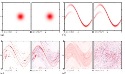
Figure 2: The phase space dynamics of the classical and quantum kicked Harper map for N = 128 and without damping (v = 1); the initial distribution is chosen according to Eq. (20) with x0=0.65, p0=0.5 and σx=σp=0.075. The left panel shows the classical

density ρn, where n is the number of iterations (using 107 particles). The right panel

shows the quantum Wigner functionWKn on a 128×128 grid with(a) n= 0, (b)n = 1,

(c) n = 3, (d) n = 10 kicks. The blue regions denote negative values of the Wigner function. A box of areah= 1/N has been included in part (a) in order to give a visual sense of the quantum scale.

[42,43,44] or the review [29] (other maps are used when discussing fluctuations about the mean later). The corresponding classical kicked Harper map exhibits a predominantly chaotic dynamics but with small regular islands. Although these islands are small, their presence leads to a significant degree of tanglement of the stable and unstable manifolds. This gives rise to a strong dependence on initial source distributions when considering correlation functions, which makes it a good test model for studying relations between classical and wave operators.

The source ˆΓ0 is chosen so that the associated Wigner distribution function takes

the form

WΓ0(x, p) =Ce

−(1−cos 2π(x−x0))/(2πσx)2−(1−cos 2π(p−p0))/(2πσp)2_{, (20)}

whereCis a normalisation constant chosen so that Tr Γ0 = 1 andσxandσp respectively

determine the variances in the x and p coordinates. For small enoughσx and σp this is

a nearly Gaussian source distribution in phase space centred on X0 = (x0, p0), and is

associated with a corresponding nearly Gaussian source correlation function Γ0(x1, x2).

The time evolution of the Wigner transformWKn of ˆKnis displayed in Fig.2and is

0

x

1

0

p

classical

0

quant.

K

x

1

0

quantum

x

1

(a)

0

x

1

0

1

p

classical

0

quant.

K

x

1

0

quantum

x

1

(b)

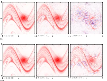
Figure 3: The stationary phase space density ρ (left) is compared with the quantum distributions WK (middle panel) and with the Wigner function of the full stationary

correlation function WΓ (right) for N = 128 and v = 0.9. The parameter for the initial

distribution arex0=0.65,p0=0.5 andσx=σp=0.075. In(b), an average over 152 different

values of the Harper map parameters (in a range of±5%) is performed in the quantum version but not in the classical version; no averaging has been done in (a) .

n as expected from Eq. (12) and detailed in Appendix A. Once the classical dynamics foliates phase space down to phase space cells of area 1/N, wave fluctuations take over and wash out the classical phase space structures, see Fig. 2d at n = 10. Note that, after several interations of the map, the classical density is stretched along the unstable manifolds of the system and tracks, for example, the folds and switchbacks in them that arise from the small islands present. Some of these features are also seen in the propagated Wigner function but the details are lost.

In Fig. 3, we compare the classical (stationary) phase space distribution ρ defined in (13) with the Wigner transforms of ˆK and ˆΓ for a damping value v = 0.9. The classical and wave results coincide remarkably well for ρ and WK even without further

averaging, see Fig. 3a, while only traces of the classical phase space structure are left for WΓ in this case. When performing a further parameter average in the Harper map,

the quantum fluctuations are suppressed and the classical phase space structure comes out more clearly, both forWK and WΓ, see Fig.3b. The fluctuations in WΓ are in both

objects ˆΓ and ˆK. We can in fact quantify the increased fluctuations in ˆΓ compared to ˆ

K as a function of v, as will be described in the next section.

The results show that the classical phase space density gives the mean value for both quantities WK and WΓ as expressed in (16). It also shows how well the classical

dynamics describes a wave operator such as WK down to a detailed description of the

complex phase space structure present in a mixed system like the kicked Harper map. Note, that the wave fluctuations due to higher iterates of the map are suppressed here due to the 10% damping (v = 0.9) introduced.

3. Fluctuations of Kˆ and Γˆ about the mean

Although ˆK and ˆΓ have the same average, the fluctuations about the mean are much greater for ˆΓ than for ˆK as illustrated in Fig.3, an effect which is greatly amplified in the weak damping limit. In this section we quantify this effect for the simple model

ˆ

T =vUˆ introduced in Sec.2.4by calculating mean values for Tr ˆΓ2and Tr ˆK2. Formally, these also provide us with variances of individual matrix elements Kij and Γij in any

given basis, using, for example,

h|Γij|2iN =

1 N2 Tr ˆΓ

2_{. (21)}

Here h·iN denotes an average over the N-dimensional basis on the space on which ˆT is

defined.

Explicit expressions can be given for these quantities, as outlined in the remainder of this section. In particular, if we average over a parameter such as frequency (or system dimension in the quantum map model), we can demonstrate that fluctuations in ˆΓ scale simply with fluctuations in ˆK, according to

hTr ˆΓ2i= 1 +v

2

1−v2hTr ˆK

2_{i. (22)}

This expression is quite general and is equally valid in chaotic and integrable limits, for example. It is also true irrespective of whether the system has time reversal symmetry or not. It provides a direct quantitative measure of the greater fluctuations seen in ˆΓ, relative to those of ˆK, as v → 1. Furthermore, we will see that the fluctuations of ˆK itself can be obtained using information that is readily available from propagation of a corresponding classical density, as performed in complex structures using the DEA method, for example.

Using (21), the scaling relationship (22) provides an equivalent scaling

h|Γij|2iN =

1 +v2

1−v2h|Kij| 2_i

N (23)

much larger than a wavelength: however, it can be shown using alternative but more involved calculations, not reported here, that these results can also be applied element by element. Finally, any statement involving such traces can be expressed also as a relation between Wigner functions. For example, (22) can also be expressed in the form,

h|WΓ(x, p)|2i=

1 +v2

1−v2h|WK(x, p)|

2_{i (24)}

using standard properties of Wigner functions. This relation provides an explicit quantitative statement of the qualitative observations made in Fig. 3.

3.1. The variance of the diagonal part Kˆ

We consider ˆK first and write Eq. (9) as

ˆ

K =

∞

X

n=0

v2nΓˆn= ∞

X

n=0

v2nUˆnΓˆ0Uˆ−n

with ˆΓn = v−2nKˆn representing the smooth n-step correlation function as in Eq. (9).

Using the cyclic permutability of the trace we may write,

Tr( ˆK2) =

∞

X

n,n0₌₀

v2(n+n0)TrhUˆn−n0Γˆ0Uˆn

0_−n

ˆ Γ0

i

(25)

=

∞

X

n,n0₌₀

v2(n+n0)A(n−n0), (26)

where

A(n) = TrΓˆ0Γˆn

is the n-step return probability. Note that A(n) = TrˆΓ0Γˆn = TrˆΓnΓˆ0 = TrˆΓ0Γˆ−n =

A(−n). After reordering the double sum, this may be written in the form

Tr( ˆK2) = 1 1−v4

∞

X

n=−∞

v2|n|A(n). (27)

So far the calculation is exact and completely independent of the classical limit.

The quantityA(n) can again be related to the classical phase space dynamics using

A(n) = TrΓˆ0Γˆn

=

k 2π

d−1Z

dX WΓ0(X)WΓn(X). (28)

We now make the approximation used in (12) that, on averaging, the fluctuations in A(n) are removed and that it may be approximated by its classical or ray-dynamical analogue, the classical phase space autocorrelation function

hA(n)i ≈Acl(n) =

Z

Here, ρ0 is the correspondingly averaged classical phase space density of the source and

ρn=Lnρ0 itsnth-reflection iterate. Then

hTr( ˆK2)i ≈ 1

1−v4

∞

X

n=−∞

v2|n|Acl(n).

For strongly chaotic systems, the autocorrelation function decays exponentially as

Acl(n)∼a0+a1exp(−γcorn), (30)

where γcor denotes the correlation exponent and a0, a1 are constants depending on the

initial densityρ0 (e−γcor typically being the 2nd largest eigenvalue of the FP operator.)

Note that, for strong damping, it suffices to know the autocorrelation functionA(n) for relatively smallnin order to compute Tr( ˆK2). In this case one finds that the exactA(n) may be well approximated by its ray-dynamical analogueAcl(n) even without averaging

and that the result above then also holds for individual maps. (Of course, the trace operation itself performs an average over basis states even if no further averaging is performed.)

3.2. The variance of the correlation function Γˆ

To get an equivalent expression for the variance of the full correlation function of the stationary wave field, ˆΓ, we start from Eq. (8), giving

ˆ Γ =

∞

X

n1,n2=0

vn1+n2_Uˆn1_Γˆ 0Uˆ−n2

from which we obtain (using cyclic permutability of the trace again)

Tr ˆΓ2 =

∞

X

n1,...,n4=0

vn1+n2+n3+n4_Tr

h

ˆ Un1_Γˆ

0Uˆ−n2Uˆn3Γˆ0Uˆ−n4

i

=

∞

X

n1,...,n4=0

vn1+n2+n3+n4_Tr

h

ˆ

Un1−n4_Γˆ

0Uˆ−n2+n3Γˆ0

i

. (31)

We argue next that, after averaging,

hTr [ ˆUnΓˆ0Uˆ−n

0

ˆ

Γ0]i=δnn0hA(n)i

due to the phase difference that one necessarily finds in contributions to ˆUn and ˆ

Un0 _{when n 6= n}0_{. On average, the sum in (31) is then dominated by terms with}

n1 −n4 =n2−n3 =n and, after reordering, we may write

hTr(ˆΓ2)i=

∞

X

n=−∞ ∞

X

n2,n4=0

v2(n2+n4)_v2|n|_hA(n)i

= 1

(1−v2₎2

∞

X

n=−∞

v2|n|hA(n)i (32)

= 1 +v

2

1−v2hTr( ˆK

as previously reported in (22). Note that this condition has been derived based on neglecting interfering contributions which are wiped out by appropriate averaging. We have not made any further assumptions about the underlying classical dynamics and the relations (22) – (24) are universal, independent of whether the system dynamics is regular, chaotic or mixed. In particular, the variance of ˆΓ always exceeds that of ˆK, only approaching the same value in the limit of strong damping, v →0.

We note that relation between wave fluctuations (as a function of energy or frequency) and classical decay rates is a well established concept and has been discussed in the context of fluctuations in scattering cross sections [45, 46] or conductance fluctuations for transport through open chaotic cavities [47], see also [48]. The relevant classical quantity is here the classical escape rate γesc, which in our setting corresponds

to the rate of dissipation γesc = −logv. A generalised treatment involving the full

spectrum of the FP operator is given in [49]. Our result highlights the influence of higher order eigenvalues of the FP operator on the variances in Eqs. (27) and (32) such as through the classical decay of correlation contributions, Eq. (30). The main result of this section is, however, the relation (33) relating the fluctuations in the ’smooth’ part,

ˆ

K, to the fluctuations in the total correlation function. Together with (17) and (29), we can now relatethe first and second moments of the distributions of both Γˆ and Kˆ to classical phase space observables such as the stationary phase space density ρ and the classical phase space autocorrelation functionAcl(n). These quantities depend of course

on the underlying classical dynamics.

3.3. Numerical illustration of fluctuations using quantum map models

The fluctuations of ˆKand ˆΓ are now illustrated using a quantum map model. As asserted in the preceding discussion, averages (27) and (32) and the corresponding variances are insensitive to the underlying symmetries and to how chaotic or integrable the system is, although the detailed distributions are not.

In this section, we use a perturbed cat map [30], in which a quantum cat map [50, 51, 52] is perturbed with a QKH map of the form used in Sec. 2.4 (see Appendix B for more details). The perturbation is large enough to break any underlying time-reversal or spatial symmetries of the quantum version of the cat map, but small enough that the overall classical dynamics is still completely chaotic. A source term Γ0 is used

which corresponds to the nearly Gaussian density given in (20), with σx = σp = 1/2.

It is centred on a period-one fixed point X0 = (x0, p0) near the origin of phase space,

which slows the short-time decay of the autocorrelation function A(n).

Corresponding numerically computed values of Tr ˆK2_{and Tr ˆΓ}2 _{are shown as circles}

10 0 10-1 10-2 10-3 10 0

10 2 10 4 10 6 10 8

1-v

Tr

Γ

2

and Tr

K

2

Figure 4: Growth in the fluctuations of ˆK and ˆΓ are illustrated as v → 1, measured respectively by TrK2 and Tr Γ2. Calculations are for a nearly Gaussian source density Γ0 driving a perturbed cat map and centred on a fixed point (of period one). Solid

curves are the averaged predictions (27) and (32) based on the classical autocorrelation function A(n). Circles and triangles are respectively evaluations of TrK2 _{and Tr Γ}2 _for

individual values of N: as v is varied, N is stepped from N = 200 to N = 400. Note that the averages (27) and (32) are independent of N: we let N change in this figure simply to give a sense of the typical variation about the predicted mean for individual maps. This aspect is illustrated more explicitly in Fig. 5

contrast, although (32) is found to be a good predictor of average behaviour, individual values of Tr ˆΓ2 _{are seen to fluctuate significantly about the mean, and to an increasing}

extent as v approaches one.

In fact, it is found in Fig. 4 that most individual values of Tr ˆΓ2 fall significantly below the mean (32) whenvis very close to one, with the average being achieved because increasingly rare individual cases arise with exceptionally large values. This can be understood simply in terms of the physics of the weakly damped resonant response of the system and is illustrated in more detail in Fig.5. Here we present fluctuations with changing N of Tr ˆΓ2 _{for the particular values v = 0.995 and v = 0.999 of the damping}

parameter, represented respectively by crosses and circles. The smallest individual values of Tr ˆΓ2 _{are insensitive to v in this illustration. Physically, these correspond}

200 300 400 10 2

10 3 10 4 10 5 10 6 10 7 10 8 10 9

N

Tr

Γ

2

Figure 5: Fluctuations in Tr ˆΓ2 are shown asN varies between 200 and 400 forv = 0.995 and v = 0.999, represented respectively by crosses and circles. The corresponding average values are shown as horizontal dashed and solid lines, respectively. The smallest values of Tr ˆΓ2 _{are insensitive to the value of v (the crosses are near the circles at the}

bottom of the graph), but the largest values change significantly as v approaches unity.

or near resonance respond very wildly to changingv and become dramatically larger as v is increased. These instances of resonant response bring the average value of Tr ˆΓ2 _up

to its predicted level (32), represented in Fig. 5by the horizontal lines.

Clearly then, the average fluctuations predicted in this paper present only a partial characterisation of the system response in the weak damping limit. A complete description demands a characterisation of the distribution of values. This lies outside the scope of the current discussion but will be reported in a future publication. The calculations in this section do provide, however, a simple characterisation of the variability of the response of the system about the mean.

4. Conclusion

The aim of this paper has been to establish and exploit an entirely wave-based analogue of this phase-space transport problem so that wave effects such as multi-path interference can be incorporated into large-scale simulations with complex and noisy forcing. We have argued that an effective platform for the calculation of such wave effects can be built on the relationship between correlation functions and Wigner functions that has been established in the contexts of quantum mechanics and optics. Two-point correlation functions provide an effective means of exploiting available information about spatial localisation and directionality of waves radiated from a noisy, complex source. They have proven to be an effective way of characterising EM emissions from electronic circuitry through direct measurement, see for example [37]. Correlation function propagators then provide a completely wave-based analogue of phase-space transport approaches such as DEA.

Importantly, this allows us to provide a statistical description of fluctuations due to interference in the response of a forced wave problem, using only information that is readily available from a direct phase-space simulation. In particular, the global variance of the wave correlation function can be described in terms of an autocorrelation function of propagated phase-space densities. In essence this allows us to boot-strap phase-space transport simulations to predict fluctuation about the mean of the response of the system, as well as the mean itself. The approach has been tested on simple quantum map models based on a representation of wave transport by boundary transfer operators, but using a framework that we believe will scale up effectively to much larger systems. Achieved results are relevant in the statistical characterisation of large vibro-acoustics and electromagnetic structures, including reverberation chambers operated at arbitrary frequencies.

Acknowledgments

We gratefully ackowledge support from from EPSRC under grant number EP/K019694/1, from the EU FP7 project MHiVec and from the EU Horizon 2020 network NEMF21.

Appendix A. The evolution of correlation functions

We will give here a derivation of Eq. (14) valid in the semiclassical limit (see also [38]). Starting from Eq. (9), we write ˆKn= ˆTnΓˆ0( ˆTn)† inx representation as

Kn(x1, x2) =

Z

dx0₁dx0₂Tn(x1, x01)K0(x01, x

0

2)(T

n

)†(x0₂, x2),

where we set K0 = Γ0 for convenience. We employ the short-wavelength approximation

Tn(x, x0)≈

k 2πi

(d−1)/2 X

α

Dα(x, x0) eikSα(x,x 0₎

of the operator ˆTn_{, where the sum index α runs over all trajectories from x}0 _{to x that}

encounter the SOS n times, while other quantities are defined as in (4) and (5) with obvious modifications. For notational compactness, the phase factorµis assumed to be absorbed into the definition of the amplitude here. Using the transformation

x1 =x+

s 2; x

0

1 =x

0

+s

0

2; (A.2)

x2 =x−

s 2; x

0

2 =x

0₋ s0

2;

and starting from the semiclassical expression (A.1), we obtain

Kn

x+ s 2, x−

s 2 ≈ k 2π

d−1Z

dx0ds0 X

αβ

Dα

x+ s 2, x

0

+s

0

2

D_β∗

x− s

2, x

0₋ s0

2

×eik(Sα(x+s/2,x0+s0/2)−Sβ(x−s/2,x0−s0/2))_K 0

x0 +s

0

2, x

0₋ s0

2

,

(A.3)

where α and β labeln-bounce orbits from x0₁ tox1 and from x02 tox2, respectively.

At this point, we need to make two crucial assumptions about the quantities of interest. First, we concentrate on the averaged response, so that orbit combinations with topologically distinct α and β, which arrive with significant noncancelling phase differences, are washed out. We are then left just with the diagonal contributions in which an orbit α coincides with an orbitβ up to a slight deformation. In the following we therefore set α = β. Second, we assume that the source has a sufficiently short correlation length that propagation can be approximated using Taylor expansions of the surviving amplitude and phase contributions, truncated at the terms

Dα

x+s 2, x

0

+s

0

2

D_α∗

x− s

2, x

0 ₋s0

2

≈ |Dα(x, x0)|2

and

Sα

x+ s 2, x

0

+ s

0

2

−Sα

x− s

2, x

0₋ s0

2

≈pα(x, x0)s−p0α(x, x 0

)s0.

Here, p0_α(x, x0) = −∂Sα(x, x0)/∂x0 and pα(x, x0) = ∂S(x, x0)/∂x [53] are respectively

With these assumptions we obtain

D

Kn

x+ s 2, x−

s 2 E ≈ k 2π

d−1Z

dx0ds0 X

α

|Dα(x, x0)|2eik(pαs−p 0

αs0)_K 0

x0+ s

0

2, x

0₋ s0

2

.

Using the definition of Dα given in (5), we may write

X

α Z

dx0|Dα(x, x0)|2{·}=

k 2π

d−1Z

dp{·},

where on the left we sum over all orbits arriving at x, labelled by initial positionx0 and topology α. On the right we reformulate the same sum as a simple integration over the momentum pat arrival (in which there is no need for the labelα sincexand puniquely determine the orbit topology). Using this reformulation of the sum we can write

D

Kn

x+ s 2, x−

s 2 E ≈ k 2π

d−1Z

dpds0

eik(ps−p0s0)K0

x0+ s

0

2, x

0₋ s0

2 = k 2π

d−1Z

dpeikps hWK0(x

0_{, p}0_)i

(A.4)

with WK0(x

0_{, p}0_{) denoting the Wigner transform of K}

0 as defined in (10). Note that

X0 = (x0, p0) in (A.4) is now a function of X = (x, p) through the relation X =ϕn_(X0_),

with ϕ defining the dynamics on the SOS (see Sec. 2.2). After applying the Wigner transformation on both sides of Eq. (A.4) and evaluating the resulting δ-function, we obtain

hWKn(X)i=

WK0 ϕ

−n_(X)

, (A.5)

which mirrors the action of the classical FP operator.

Appendix B. Conventions for quantum maps

Here we summarise the quantum maps used in Secs. 2.4 and 3.3 to test correlation function propagation. We use maps defined on a toral phase space with unit period in each of the phase space coordinates x and p.

We begin with the classically-defined kicked map defined by

x=x0+G0(p0)

p =p0−F0(x), (modulo 1)

and F0(x) = bsin 2πx and a = −2b = 2/π, in which case the map is a kicked Harper map, which will be the nomenclature we use henceforth. These maps provide generic examples with predominantly chaotic dynamics mixed with small regular islands for the chosen parameter values.

The corresponding quantum map is then defined on a Hilbert space of dimension N = 1/(2π_~) such that

ˆ

UQKH = e−2πNiF(ˆx)e−2πNiG( ˆp).

The geometry of phase space is reflected in the detailed quantisation of the position and momentum operators ˆx and ˆp, and on the boundary conditions imposed on quantum states. We can use a position basis ˆx|xii = xi|xii, with quantised positions

xi = (i+αx)/N, whose index i runs over i = 0,· · · , N − 1. Alternatively, we can

use a momentum basis ˆp|pii = pi|pii on the same index set with quantised momenta

pi = (i+αp)/Nand related to the position basis byhxl|pji= e2πNixlpj/ √

N. The shiftsαx

and αp are determined by the boundary conditions satisfied by states under translation

across the torus. The direct wavefunctionψ(xi) =hxi|ψisatisfiesψ(xi+1) = e2πiαpψ(xi).

The momentum representation ϕ(pi) = hpi|ψi satisfies ϕ(pi+ 1) = e−2πiαxϕ(pi). All of

the maps used in this paper use eitherαx =αp = 0 orαx =αp = 1/2 and, in particular,

Figs. 2-3 assumedαx =αp = 0.

Alternatively, cat maps and their quantisations provide examples of fully chaotic, hyperbolic dynamical systems. Quantisations of the simple cat map exhibit nongeneric degeneracies but these can be removed by perturbations which retain the fully chaotic dynamics. In particular, we use a perturbed cat map

ˆ

UPC = ˆUCUˆQKH,

where ˆUQKH is a quantum kicked Harper map and ˆUC, defined by

hxj|UˆC|xli=

1

√

Ne

2πNi(x2

j−xjxl+x2l/2),

quantises the (unperturbed) cat map

x=x0+p0

p =x0+ 2p0 (modulo 1).

This quantisation is well-defined for even N with αx = αp = 0 and for odd N with

αx =αp = 1/2. The QKH map used for the numerical illustration in Sec. 3.3 was also

of this form with G0(p) = asin 2πp, F0(x) = −bsin 2πx and a = b = 0.1. This choice completely eliminates symmetries in the combined map, while presenting a small enough perturbation of the cat map that the dynamics is fully chaotic.

References

[2] Wright M and Weaver R 2010 New Directions in Linear Acoustics and Vibration, Cambridge: Cambridge University Press.

[3] Gradoni G, Yeh J-H, Xiao B, Antonsen T M, Anlage S M, Ott W 2014, Wave Motion51, 606-621. [4] Gros J-B, Legrand O, Mortessagne F, Richalot E, Selemani K 2014, Wave Motion 51, 664-672. [5] Guhr T, M¨uller-Groeling A and Weidenm¨uller H A 1998, Physics Reports299, 189-428.

[6] St¨ockmann H J 1999Quantum Chaos – An Introduction, Cambridge: Cambridge University Press. [7] Haake F 2001 Quantum Signatures of Chaos, 2nd edn, Berlin:Springer.

[8] Mehta M L 2004Random Matrices, 3rd edn, New York: Academic Press. [9] Bohigas O, Giannoni M J and Schmit C 1984, Phys. Rev. Lett.52, 1. [10] Creagh S C, Ben Hamdin H and Tanner G 2013, J. Phys. A46, 435203.

[11] Gradoni G, Creagh S C, Tanner G, Smartt C and Thomas D W P 2015, New J. Phys.17, 093027. [12] Hillery M, O’Connell R, Scully M and Wigner E 1984Physics Reports 106121-167.

[13] Dragoman D 1997Progress in Optics XXXVII (Elsevier).

[14] Torre A 2005Linear Ray and Wave Optics in Phase Space: Bridging Ray and Wave Optics via

the Wigner Phase-Space Picture (Elsevier Science).

[15] Alonso M A 2011 Adv. Opt. Photon.3272–365.

[16] Littlejohn R G and Winston R 1993 J. Opt. Soc. Am. A102024-2037.

[17] Winston R, Kim A D and Mitchell K 2006 Journal of Modern Optics532419-2429. [18] Dittrich T and Pach´on L A 2009 Phys. Rev. Lett.102(15) 150401.

[19] Berry M V 1977 J. Phys. A: Math. Gen.102083.

[20] Hemmady S, Antonsen T M, Ott E and Anlage S M 2012 IEEE Trans. Electromag. Compat.99

1.

[21] Creagh S C and Dimon P 1997 Phys. Rev. E55(5) 5551-5563. [22] Hortikar S and Srednicki M 1998 Phys. Rev. Lett.80(8) 1646-1649. [23] Weaver R L and Lobkis O I 2001 Phys. Rev. Lett.87(13) 134301. [24] Urbina J D and Richter K 2006 Phys. Rev. Lett.97(21) 214101. [25] Marcuvitz N 1991 Proceedings of the IEEE791350-1358. [26] Tanner G 2009 Journal of Sound and Vibration32010231038.

[27] Chappell D J, Tanner G, L¨ochel D and Søndergaard N 2013 Proceedings of the Royal Society A: Mathematical, Physical and Engineering Science46920130153.

[28] Gradoni G, Creagh S C, Tanner G, Smartt C, Baharuddin M H, Thomas D W P, 2015 IEEE, Benevento, 2015, 220-224.

[29] Artuso R,Kicked Harper model, Scholarpedia,

http://www.scholarpedia.org/article/Kicked_Harper_model. [30] Creagh S C 1994,Chaos5, 477-493.

[31] Bogomolny E B 1992 Nonlinearity5805.

[32] Tanner G and Søndergaard S 2007, Phys. Rev. E75036607.

[33] Prosen T 1994 J. Phys. A: Math. Gen. 27 L709L714; Prosen T 1995 J. Phys. A: Math. Gen. 28 41334155.

[34] Rouvinez C and Smilansky U 1995 J. Phys. A 28 77103. [35] Prosen T 1996 Physica D 91 244277.

[36] Doron E and Smilansky U 1992 Nonlinearity51055-1084.

[37] Smartt C, Thomas D W P, Nasser H, Baharuddin M, Gradoni G, Creagh S C and Tanner G 2015, IEEE International Symposium on Electromagnetic Compatibility (EMC), Dresden 2015, IEEE, 953-958.

[38] Manderfeld C, Weber J and Haake F 2001, J. Phys. A: Math. Gen.3498939905.

[39] Cvitanovi c P, Artuso R, Mainieri R, Tanner G, Vattay G, Whelan N, Classical and Quantum

Chaos - A Cyclist Treatise, http://chaosbook.org/.

[40] Chappell D J and Tanner G 2014, CHAOS 24, 043137.

[43] Geisel T, Ketzmerick R, and Petschel G 1991, Phys. Rev. Lett.66, 1651-1654; Geisel T, Ketzmerick R and Petschel G 1991, Phys. Rev. Lett.673635 - 3638.

[44] Lima R and Shepelyansky D 1991, Phys. Rev. Lett.671377- 1380. [45] Bl¨umel R and Smilanksy U 1988, Phys. Rev. Lett.60477-480.

[46] Doron E, Smilanksy U and Frenkel A 1990, Phys. Rev. Lett.65 3072-3075. [47] Jalabert R A, Baranger H U and Stone A D 1990, Phys. Rev. Lett.65 2442-2445. [48] Baranger H U 1995, Physica D8330-45.

[49] Agam O 2000, Phys. Rev. A611285-1298.

[50] Hannay J H and Berry M V 1980, Physica 1D 267 - 290. [51] Keating J P 1991, Nonlinearity4309-341.

[52] Agam O and Brenner N, 1995, J. Phys. A28, 1345 - 1360.