Bath induced coherence and the secular approximation

P. R. Eastham,1 P. Kirton,2 H. M. Cammack,2 B. W. Lovett,2 and J. Keeling2

1

School of Physics and CRANN, Trinity College Dublin, Dublin 2, Ireland.

2_{SUPA, School of Physics and Astronomy, University of St. Andrews, KY16 9SS, U.K.}

Finding efficient descriptions of how an environment affects a collection of discrete quantum systems would lead to new insights into many areas of modern physics. Markovian, or time-local, methods work well for individual systems, but for groups a question arises: does system-bath or inter-system coupling dominate the dissipative dynamics? The answer has profound consequences for the long-time quantum correlations within the system. We consider two bosonic modes coupled to a bath. By comparing an exact solution against different Markovian master equations, we find that a smooth crossover of the equations-of-motion between dominant inter-system and system-bath coupling exists – but requires a non-secular master equation. We predict a singular behavior of the dynamics, and show that the ultimate failure of non-secular equations of motion is essentially a failure of the Markov approximation. Our findings support the use of time-local theories throughout the crossover between system-bath dominated and inter-system-coupling dominated dynamics.

I. INTRODUCTION

A Markovian system is one in which the future time evolution depends only on the current state, and not on its history [1]. In the context of open quantum systems, Markovianity generally implies that the reduced density operator obeys a first-order differential equation. This class of theory has been developed for many years, is applied to a vast range of systems, and provides our un-derstanding of quantum damping and decoherence [2]. Recent work, however, presents it with challenges. The development of solid-state quantum emitters, such as sin-gle and coupled quantum dots [3, 4] and superconducting-qubit cavities [5, 6], demands theories capable of treat-ing driven or coupled systems damped by complex struc-tured baths [7–11]. Such theories reveal, among other ef-fects, the possibility of engineering the reservoirs to con-trol quantum coherence [12, 13]. They show that under appropriate conditions both quantum coherence [14] and entanglement [15–17] can survive indefinitely, even for high temperature baths [18, 19].

These problems do not necessarily elude treatment by a time-local theory, i.e., a (Markovian) quantum mas-ter equation. Such theories accurately reproduce the intensity-dependent damping of quantum dots in a struc-tured reservoir [4, 20, 21], for example, and provide recent predictions of bath-induced coherence [14] and entangle-ment [16, 17]. However, there are several master equa-tions consistent with, and derivable from, the assumption of weak coupling [22, 23]. Furthermore, master equations are often postulated phenomenologically, by choice of the jump operators in the Lindblad form. For problems with multiple oscillators and structured baths this choice is not straightforward, with different choices plausible in differ-ent limits. Nor is it innocdiffer-ent: differdiffer-ent forms of master equation lead to different behavior [24]. Thus it is impor-tant to establish which, if any, of the various time-local theories is correct.

In this paper we address this question by studying an exactly-solvable model, and comparing the exact solution

against various time-local theories. We consider a model of two bosonic modes, ˆψa,b, with frequencies ωa,b, cou-pled to a thermally-occupied bath with spectral density

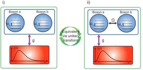
J(ν). This model has a non-trivial Hamiltonian, multi-ple degrees-of-freedom, and frequency-dependent damp-ing, yet is exactly solvable. We consider the general case where the natural frequencies ωa,b differ and the bath couples to a superposition of modes,ϕ∗_aψaˆ +ϕ∗_bψbˆ , and calculate the evolution of the coherence, hψˆ_a†ψbˆ i. We find a complex behavior with multiple regimes, visible in Fig. 2, reflecting the competing effects of the system Hamiltonian and the coupling to the bath. We will com-pare the exact solution with time-local theories, and so identify those which correctly capture such physics. This allows us to establish their validity in a generic prob-lem, and avoids the difficulty inherent in studying only approximate theories.

A physical issue we will address is the appropriate form of dissipator for systems with multiple compo-nents. Two different forms are expected on physical grounds [25]. In the case of the two-oscillator model it is clear that at resonance, ωa = ωb, the damping can

depend only on the pattern of coupling to the baths. Thus we expect collective decay, described by a Lind-blad formLc= Γ↓L[ϕa∗ψˆa+ϕ∗bψˆb] + Γ↑L[ϕaψˆa†+ϕbψˆb†],

where L[ ˆψ] is the standard dissipator with jump oper-ator ˆψ [2]. Far off-resonance, however, we expect indi-vidual decay terms,Li =P

i=a,bΓ

↓

iL[ ˆψi] +

P

iΓ

↑

iL[ ˆψ

†

i].

implies that some useful effects – specifically the protec-tion of coherence against the bath – are critically sensitive to microscopic parameters. Moreover, while the crossover can be treated by a time-local theory, this theory is not a Lindblad form with the required positive rates. The use of such forms is the subject of ongoing debate, since they are not completely positive maps [26]. This means that they can lead to unphysical density operators, with negative eigenvalues.

A methodological issue in this debate is the procedure of secularization. This amounts to removing from the equations-of-motion those terms which are time depen-dent in the interaction picture. It was used in some of the earliest work on quantum damping by Bloch and Wangsness [27], but was then argued to be unneces-sary by Redfield [28] as well as Bloch [29]. That po-sition was challenged by the subsequent Lindblad theo-rem [30]: as argued by D¨umcke and Spohn [23], secu-larization is required to reach a description where Lind-blad’s theorem ensures positivity of the density operator. Indeed, Lindblad’s theorem guarantees that the density operator will remain positive even when there is entan-glement with an auxiliary system, a criterion known as complete positivity [2]. Secularization, which leads to a completely positive theory, is clearly appropriate when the interaction-picture time dependence is fast, since off-diagonal terms then rapidly average to zero. In our case, this is far off-resonance, and secularization indeed leads from the Bloch-Redfield equation to the form Li. How-ever, for a tunable system it may occur that the the time-dependence in the interaction picture becomes slow in certain regimes, i.e., approaching resonance, so that sec-ularization becomes inappropriate. An interesting im-proved version of the secularization procedure is studied in Ref. [26].

Recently, the necessity of secularization has been ques-tioned [31, 32]: Simulations indicate that for time evo-lution following an initially prepared separable state, secularization (and even a Lindblad form for the equa-tion of moequa-tion) can be unnecessary for positivity [33], and even complete positivity [34], in particular for time-convolutionless [2] and Nakajima-Zwanzig [35, 36] ap-proaches. Stronger statements to this effect have also been made by Hell et al. [37], noting that a conserva-tion law [38] is violated by secularized theories — we discuss this sum rule in detail further below. The ques-tion of how the operator form of time-local and non-Markovian approaches are related is reviewed by Kar-lewski and Marthaler [39]. Our focus in this paper is, however, on cases where a time-local description is suffi-cient. This will enable us to explore the entire parameter space of a model, and identify the regions where Bloch-Redfield equations predict physical behavior. We will show that, although the damping is not of Lindblad form, the anticipated unstable behavior does not occur within the domain of applicability of the theory – specifically, so long as the bath remains Markovian.

The exact results we present are restricted to only a

subset of possible initial density matrices. We take as ini-tial conditions a thermal state of the bath and the ground state of the two oscillators. The reduced density matrix is then Gaussian at all times, and so completely charac-terized by its second moments. Thus we will be able to establish whether the Bloch-Redfield equations are accu-rate and physical from the dynamics of those moments alone. This does not, however, rule out inaccurate or even unphysical behavior for arbitrary (non-Gaussian) initial density matrices.

Within the scope of coupled open quantum systems, a particular motivation for our work comes from the timely theory of “weak lasing” [40] introduced in the context of polariton condensates. The idea presented is that for modes which are close to resonance the (dissi-pative) radiative coupling can select which linear com-bination of modes lases (condenses) first. These works started from a phenomenological description of radiative coupling, in which collective dissipation terms are intro-duced by hand. In the following we will see, however, that the effects of collective dissipation terms are strongly de-pendent on whether the individual modes are degenerate or not. Our work does not consider the general prob-lem with both drive and dissipation, but the results we present for coupling to a single bath suggest there may be a need to re-examine how weak-lasing evolves where ra-diative coupling selects superpositions of non-degenerate modes.

The remainder of this paper is structured as follows. In Sec. II we describe the model. In Sec. III we present the exact solution, and discuss its behavior. In Sec. IV we discuss the comparison with the Bloch-Redfield equation and the na¨ıve Lindblad forms mentioned above. We also identify the parameter regimes where the Bloch-Redfield equation gives physical behavior. In Sec. V we develop an alternative to the Bloch-Redfield equation, and show it to be an improvement both numerically and analytically. In Sec. VI we give the generalization of our work to the case of multiple baths. Finally, in Sec. VII, we give our conclusions.

II. MODEL

The two bosons and the common bosonic bath are rep-resented by the Hamiltonian ˆH = ˆHS+ ˆHSB+ ˆHB. The

system Hamiltonian is ˆHS =ωaψˆa†ψˆa+ωbψˆb†ψˆb, in terms

of bosonic annihilation operators ˆψi. The bath Hamilto-nian is ˆHB =Piωicˆ†iˆci, whereci annihilates a boson in

modei. The system-bath coupling takes the form

ˆ

HSB= (ϕ∗aψˆa†+ϕ∗bψˆ

†

b)

X

i

gicˆi+ H.c.. (1)

The complex coefficients ϕi determine which pattern of

system operators the bath couples to, and gi captures

the overall coupling to modei. We will assume the bath has a continuous density of states parameterized by the spectral densityJ(ν) =P

ig

2

Since this model is a linear system of coupled harmonic oscillators it is exactly solvable. The exact solution for a single harmonic oscillator coupled to a bath [41] is well-known [42]. The extension to the case of two identical oscillators coupled symmetrically to a bath can be found in Ref. [43], and has been used to test master equation approaches [31]. In this special case the normal modes exactly match the pattern of bath coupling. The anti-symmetric mode then decouples from the bath, imme-diately reducing the problem to one damped oscillator and one undamped one. The dynamics of entanglement in this case was studied by Paz and Roncaglia [15], who showed that the undamped mode allows entanglement to persist indefinitely. We consider a more general problem, including detuning ∆ = (ωa−ωb)/26= 0, which prevents

such a decoupling and leads to finite lifetimes.

The existence of finite lifetimes at non-zero ∆ can be understood by observing that the model above is equivalent to a system of two coupled oscillators, one of which is coupled to a bath, i.e., the Hamiltonian

ˆ

HS = ωcψˆ†cψˆc +ωdψˆ

†

dψˆd+ Ω ˆψ†cψˆd + H.c. with ˆHSB =

ˆ

ψ†_cP

igiciˆ + H.c.. This mapping follows on transforming

this latter problem to a basis in which ˆHS is diagonal. These two equivalent problems are illustrated schemati-cally in Fig. 1. We will use the basis of Eq. (1) in the following; the results of the other problem can be simply extracted by the appropriate rotations.

In what follows, we consider the time evolution of the observables Fij(t) ≡ hψˆi†ψˆji, focusing in particular on

the coherenceFab(t) which, as mentioned earlier, distin-guishes collective from individual decay. Furthermore, these observables fully characterize the density matrix for the initial conditions we consider; it is Gaussian, so that higher moments are related to the Fij by Wick’s

theorem. We first present the exact solution and dis-cuss its observed properties, before considering the (non-secularized) Bloch-Redfield (BR) equation of motion. We will show both analytically and numerically that this ap-proach reproduces the exact solution, while either of the na¨ıve Lindblad master equations fail to reproduce the exact results.

III. EXACT SOLUTION

The exact time evolution can be readily found by us-ing a Laplace transform to write the system operators in terms of the t = 0 bath operators, and then evaluating

Fij(t) using thermal correlations for the bath operators

att= 0. With the oscillators in the ground state att= 0 we find:

Fij(t) =

Z

dνJ(ν)nB(ν)Wi∗(ν, t)Wj(ν, t), (2)

W_i(ν, t) =ϕi

Z _dζ

2π

(ω¯i−ζ)e−iζt

(ν−ζ−i0)d(ζ+i0), (3)

J(ν)

ν

ωa

Equivalent via unitary transform

Boson a Boson b

J(ν)

ν Boson a Boson b

Ω

g

i) ii)

g

ωb ωa ωb

FIG. 1. (Color online) Cartoon of the system we consider: (i) two bosonic modes of frequenciesωa, ωbcouple collectively to

a single bath. As illustrated, we take a super-Ohmic bath with an exponential cutoff when an explicit form is required. (ii) the equivalent problem of two coupled modes with a bath coupling to only one of the modes.

whereω¯a=ωband vice versa,nB(ν) is the Bose-Einstein

distribution function, and d(ζ) = −(ωa−ζ)(ωb−ζ) + iK∗(ζ)[|ϕa|2_{(ωb−ζ)+|ϕb|}2_{(ωa−ζ)] is the denominator of} the retarded Green’s function. Here we have introduced

K(ζ), the analytic continuation of the damping rate to the lower half planeK(ζ) =iR

dxJ(x)/(x−ζ+i0). For realζ the real part ofK(ζ) is the spectral density, while the imaginary part follows from a Kramers-Kronig rela-tion. In the numerical results which follow we use the form of spectral density illustrated in Fig. 1. For nu-merical evaluation, it is computationally more efficient to write this as a convolution:

Fij(t) = Z t

0

dτ

Z t

0

dσDi(t−τ)∗Dj(t−σ)α(σ−τ), (4)

Di(t) =ϕi

Z _dζ

2π

(ω¯_i−ν)e−iζt

d(ζ+i0) , (5)

α(τ) = Z

dνJ(ν)nB(ν)e−iντ. (6)

One may readily check that this is equivalent to Eqs. (2,3).

A. Behavior near degeneracy

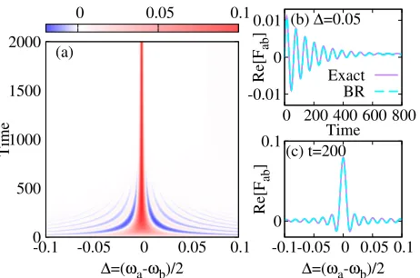
Using the above expressions, one may directly find how the coherence evolves with time, as the detuning ∆ = (ωa−ωb)/2 changes; this is shown in Fig. 2. As is

0 500 1000 1500 2000

-0.1 -0.05 0 0.05 0.1

Time

∆₌₍ω

a-ωb)/2

0 0.05 0.1

(a)

-0.01 0 0.01

0 200 400 600 800

Re[F

ab

]

Time Exact

BR

(b) ∆_=0.05

0 0.1

-0.1-0.05 0 0.05 0.1

Re[F

ab

]

∆₌₍ω

a-ωb)/2

(c) t=200

FIG. 2. (Color online) (a) Evolution of coherence Fab with

time (vertical) and detuning (horizontal), found from the ex-act solution. We use a super-Ohmic density of states with an exponential cutoff,J(ω) =J0ez−zω/ω0_(ω/ω0)z_{. This form is}

written such that its peak value is atω=ω0, andJ(ω0) =J0. We choosez = 3, and we measure all energies and times in units such thatωa= 1. In these units ω0 = 0.9, J0 = 0.001,

and the thermal occupation is controlled bykBT = 0.52. The

horizontal axis is the detuning, found by varyingωbfor fixed ωa. (b) Vertical slice at ωb= 0.9 corresponding to ∆ = 0.05,

showing comparison between exact and Bloch-Redfield theo-ries. (c) Horizontal slice att= 200. In the secularized theory the coherenceFab= 0 for all times.

The origin of the discontinuity at degeneracy is the emergence of a slow mode, whose lifetime diverges as ∆→0. The decay rates of oscillations can be extracted from the poles ζ0 of the the Keldysh Green’s function, i.e. solutions ofd(ζ0_{) = 0. Writingωa,b = Ω±∆ leads to} an expression:

0 = ∆2+ ∆(|ϕa|2_{− |ϕb|}2_)iK∗_(ζ0₎

−(Ω−ζ0) Ω−ζ0−iK∗(ζ0)[|ϕa|2_+|ϕb|2_]

. (7)

At ∆ = 0, the first line vanishes so it is clear that there is a poleζ0_{= Ω, which is real and so entirely undamped.} This has a simple physical interpretation: at ∆ = 0, there is no coupling between the combinationP

iϕiψˆiand the

orthogonal combination of fields. As such, the orthog-onal combination is entirely undamped, and maintains its original state. With non-zero detuning, beating be-tween the modes ˆψi=a,b means the orthogonal

combina-tion evolves intoP

iϕiψiˆ with time, and is thus damped.

Considering small ∆ perturbatively gives:

=[ζ0] =− 4∆ 2_|ϕ

a|2|ϕb|2

(|ϕa|2_+|ϕb|2₎3

K0(Ω)

|K(Ω)|2 +O(∆

3_{). (8)}

This explains the Gaussian form of the singular response visible in Fig. 2: we expect Fab(∆, t→ ∞)∼Fab¯ (∆) +

Cexp(−α∆2t) at larget, whereC, αare constant factors and ¯Fab(∆) is a smooth function.

B. Late time asymptotes

The long-time asymptotes of the observables can be ob-tained from the pole structure of the Laplace-transform solution [44]. For late times, Wi(ν, t) simplifies signifi-cantly because the pole at ζ = ν −i0 lies on the real axis and so has a vanishing decay rate, while the poles ofd(ζ+i0) are generically off axis and so have decayed at late times. Thus Wi(ν, t → ∞) = [−ie−iνt]ϕi(ω¯_i −

ν)/d(ν+i0). This gives a simplified expression

Fij(∞) =ϕ∗_iϕ_j

Z

dνJ(ν)nB(ν)(ω¯i−ν)(ω¯j−ν) |d(ν+i0)|2 . (9) As can just be seen in Fig. 2, away from the resonance point, the off-diagonal coherence decays at late times to a small value, but not strictly to zero. However, if the bath density of states and occupation are strictly flat, i.e. if J(ν) =J0, nB(ν) = n0, then one may show that the asymptotic valueFij(∞) vanishes for ∆6= 0. In this

case Eq. (9) simplifies considerably, as K(ν) = πJ0 for a flat bath, so d(ν +i0) becomes a simple polynomial. This integral then has only four simple poles, and one may readily check that it exactly vanishes – except at

ωa=ωb, where two of the poles coincide and cancel with

the zeros of the numerator. The small residual coherence that exists away from resonance in Fig. 2 is thus due to the frequency dependence ofnB(ν), J(ν).

IV. BLOCH-REDFIELD APPROACH

So far, we have seen that the exact solution of the bosonic problem does show a crossover between strong coherence at degeneracy and weak coherence, due to a frequency-dependent spectral density, away from degen-eracy. However, this crossover occurs as a function of time, with coherence surviving over a range αt'∆−2_. A similar quadratically diverging timescale is found in the V-type system [14]. We now turn to consider whether the behavior of the coherence, and other observables, can be reproduced by a time-local master equation.

reach canonical equilibrium. More generally, since Lc

is parameterized by one pair of forward/backward rates, it cannot account for the presence of two frequencies in the dynamics at which the bath should be sampled. As can be seen from Fig. 2, this occurs above a critical value of the detuning. Thus this model cannot possibly be ac-curate in this regime, unless the bath and its occupation are flat.

Thus, neither na¨ıve form of dissipator can give a full account of problems with multiple system frequencies and structured baths, particularly if one seeks to ana-lyze coherence. Unfortunately many interesting prob-lems in solid-state quantum optics fall in this class, as discussed in the introduction. We will now show, how-ever, that a Bloch-Redfield equation does reproduce the correct behavior, as long as one does not secularize the final result. Such an approach is frequently stated to be invalid, as it leads to negative rates and instabilities. We will however show analytically that such instabilities oc-cur in a much restricted parameter regime, and, in fact, only when the Markov approximation breaks down. The non-secularized theory is, also, often argued to be in-valid on the related grounds that it is not a completely positive map, and may not even be a positive one. We will however show analytically that, although the map is not positive, it preserves positivity for almost all Gaus-sian states. Furthermore, we find numerically that these states soon dominate under the time evolution, even if dangerous ones are present in the initial conditions.

Following the standard method [2] one finds the master equation has the form:

∂tρ=−i[ ˆH, ρ] +X

ij

L↓_ijϕ∗_iϕ_j2 ˆψ_jρψˆ_i†−[ρ,ψˆ_i†ψˆ_j]+

+X

ij

L_ij↑ϕ_iϕ∗_j2 ˆψ_j†ρψˆ_i−[ρ,ψˆ_iψˆ†_j]+

. (10)

Here the Hamiltonian includes Lamb shifts ˆH = ˆHS − P

ijhijϕ

∗

iϕjψˆ

†

iψˆj. The matricesLσ∈↓,↑, hcan be written

in a compact form,

Lσ=

Kaσ0 K¯σ0 ±iδKσ00

¯

K_σ0 ∓iδK_σ00 K_b,σ0

(11)

h=

K_a00 K¯00−iδK0

¯

K00+iδK0 K_b00

, (12)

with the upper (lower) signs in Eq. (11) for L↓ (L↑). Here we have introduced several new pieces of no-tation. We have used the shorthand Ki = K(ωi)

in terms of the Hilbert transform (analytic continua-tion) defined previously, and have also defined Hilbert transforms of the excitation (absorption) rate Ki↑ =

iR

dξnB(ξ)J(ξ)/(ξ−ωi+i0), and de-excitation (emission) rateKi↓=iR dξ(nB(ξ) + 1)J(ξ)/(ξ−ωi+i0). Note that

this meansKi=Ki↓−Ki↑. Primes signify real and imag-inary parts and ¯X = (Xa+Xb)/2, δX = (Xa−Xb)/2.

While Eqs. (10–12) fully describe the equations of mo-tion, it is more convenient to use the (closed) set of

equa-tions of motion for the quantitiesF_ij derived from these master equations. In order to simplify these equations, it is convenient to note that the phase of the complex coefficientsϕi can be eliminated by a phase twist of the

original operators, and we thus assume ϕi is real from

hereon. We may then define the vector of real quantities

f = (F_aa, F_bb,2F_ab0 ,2F_ab00)T and produce an equation of motion∂tf =−Mf+f0 where

M=



 

2ϕ2

aKa0 0 ϕaϕbKb0 ϕaϕbKb00

0 2ϕ2_bK_b0 ϕbϕ_aK_a0 −ϕbϕ_aK_a00

2ϕaϕ_bK_a0 2ϕbϕ_aK_b0 Γ0 −E0 −2ϕaϕbK

00

a 2ϕbϕaKb00 E0 Γ0 

 ,

(13) with E0 = (ωb −ϕ2bK

00

b)−(ωa −ϕ2aKa00), and Γ0 =

ϕ2

aKa0 +ϕ2bKb0. None of these rates depend on the

bath mode occupations, however the constant vector

f0 = 2(ϕ2aKa,0 ↑, ϕ 2

bKb,0↑, ϕaϕb2 ¯K↑0, −ϕaϕb2δK↑00)

T

in-volves the excitation rate, so that populations are pro-portional to the bath occupations as expected.

The result of time evolving this closed set of equations is shown in Fig. 2(b,c), and clearly compares very well to the exact solution. Moreover, we can easily see that secularizing this set of equations, as is often claimed to be a crucial step [23], could only decrease the agreement: secularization can be shown to be equivalent to setting all terms involving the productϕaϕbto zero, thus

remov-ing the off-diagonal blocks of Eq. (13) and the last two elements of the vectorf0. This then makes the coherence

Fab(t) identically zero. This is as expected for a secular theory: a non-zero detuningωa 6=ωb means the master equation contains no cross terms between modesa, band thus no coherence arises. Note that the coherence in the secular theory is identically zero, whereas that in the ex-act result decays to a small value after the time 1/(α∆2), see Eq. (8). We can thus identify this timescale as that controlling the secular approximation.

A. Stability of time evolution

The frequently stated reason [23] for secularizing the equation of motion is that it is required to ensure the equation is of Lindblad form with positive rates, i.e. that the master equation take the form ˙ρ =−i[H, ρ] + P

iλi(2 ˆΛiρΛˆ

†

i −[ ˆΛ

†

iΛˆi, ρ]+) withλi≥0. This is desired so that Lindblad’s theorem can guarantee complete pos-itivity of the density matrix. In addition, negative de-cay rates may lead to exponentially growing observables. Despite its near-perfect match to the exact solution, our non-secularized equation clearly fails these requirements. Eq. (10) can be put into Lindblad form by diagonalizing the matricesLσ∈↑,↓ _{in Eq. (11), however the eigenvalues} areλσ = ¯Kσ0 ±Sσ whereSσ2 = ( ¯Kσ0)2+|δKσ|2≥( ¯Kσ0)2.

This means that except when δKσ = 0, one rate is

applying such a theory.

In our problem, we are able to find precise conditions under which the negative rates in the Lindblad form cause a practical problem. Operationally, our problem is to solve the four linear coupled equation for the com-ponentsFij. This method will fail if the matrixM has negative eigenvalues. For a Gaussian problem such as the one we consider here this condition is in fact the only practical consideration; all higher moments factorize by Wick’s theorem and so positivity of the eigenvalues ofM

ensures the dynamics remains bounded. Remarkably, the eigenvalues of Mcan be found in closed form. They are

Mφi=µiφi with

µi =<[ ˜Ka+ ˜Kb]±

p

<[Q]± |Q|, (14)

Q= 2 ˜KaKb˜ +1 2 h

˜

Ka−Kb˜ +i(ωa−ωb)i 2

where ˜Ki = ϕ2

iKi. It is clear that when ωa =ωb, one

finds Q = [ ˜Ka + ˜Kb]2/2, which means <[Q] +|Q| =

(<[ ˜Ka + ˜Kb])2. Thus the Bloch-Redfield form recovers

the fact there is a zero eigenvalue at degeneracy.

From this closed form we may check that the eigenval-uesµi remain positive (stable) as long as

2∆2K˜_a0K˜_b0+ ∆( ˜K_a0 + ˜K_b0)( ˜K_a0K˜_b00−K˜_b0K˜_a00)>0. (15) The first term is always positive, and thus instability re-quire two conditions: Firstly, it rere-quires that ∆( ˜K0

aK˜b00−

˜

K_b0K˜_a00) < 0, placing a constraint on the frequency de-pendence of J(ν) — typically an instability is hard to achieve if J(ν) has only a single peak, but is possible for a multi-peaked structure. Secondly, and more im-portantly, in order that the second term in Eq. (15) can dominate, it is necessary that dK(ω)/dω must be large enough — this corresponds directly to requiring that the spectral density should vary significantly on a scaleJ(ω), i.e. that the memory time of the bath is comparable to the damping timescale. If such a condition is satisfied, then the Markov approximation isa priori invalid.

To summarize, as long as the Markov approximation is valida priori – i.e. the bath memory time is short com-pared to damping time – then the eigenvalues of M are positive and the solution is stable. This result shows that Markovianity is, for this problem, a sufficient condition for stability. This is despite the Lindblad matrices L↑,↓ always having negative eigenvalues, except at resonance.

B. Comparison to exact solution near degeneracy

We have already seen the numerical agreement between this BR treatment and the exact result in Fig. 2. We may note that near resonance one can compare the per-turbative solution of the exact problem to a perper-turbative expansion of the BR eigenvalues. Starting from Eq. (14), and expanding up to quadratic order in ∆ and δK, one

finds:

µ0= 8ϕ2

aϕ2b∆

2_K¯0 (ϕ2

a+ϕ2b)3|K¯|2

−8ϕ 2

aϕ2b∆( ¯K0δK00−δK0K¯00)

(ϕ2

a+ϕ2b)2|K¯|2

+O(∆3). (16)

Recall that δK depends on the detuning, vanishing at least linearly as ∆→0, so that the second term is at least second-order in ∆. This eigenvalue can be compared to the exact perturbative result by referring back to Eq. 8 and noting that µexact

0 = −2=[ζ0]. The factor of two appearing here is becauseµcorresponds to the eigenvalue of the population equation, whereas the pole in Eq. 8 gives the decay of fields ˆψi.

Comparing Eq. (8) to Eq. (16) one sees that the leading-order term in K(ω) is correct, but the second term in Eq. (16) is not there in the exact solution. The second term is however dependent on the derivative of the functionK. Thus one finds again that the BR theory is correct as long as the Markovian approximation holds, i.e. as long as the derivative of the density of states is sufficiently small.

C. Positivity of time evolution

As we have seen, the Bloch-Redfield time evolution is stable, and has the correct steady-state, so long as the Markovian approximation is justified. This rules out the most dramatic pathologies that could arise from the negative rates, and suggests that the dynamics will not stray far from the correct behavior. This is consistent with the essentially perfect agreement seen numerically. We now consider a related issue, of the extent to which the negative rates lead to unphysical density matrices with negative eigenvalues.

We first summarize some standard definitions [2]. An operator is positive if all its expectation values are posi-tive, and a map is positive if it is between positive opera-tors. Since density operators are positive the exact time-evolution superoperator, which is a map between density matrices, is positive. The secularized master equation in fact satisfies the stronger criterion of complete posi-tivity, which corresponds to positivity in the presence of arbitrary entanglement with an auxiliary system.

The map given by Eq. (10) can be shown to be non-positive specifically because of the negative eigenvalues of the Kossakowski matrices L↑,↓_{. To demonstrate this} we suppose thatL↓_{has a negative eigenvalue, and work} in its diagonal basis. We denote the field operator corre-sponding to the unstable (stable) eigenvector by ˆψc ( ˆψd),

so that there will be terms in Eq. (10) of the form

r2 ˆψcρψˆ†c−[ρ,ψˆ†cψˆc]+

(17)

for all pairsi, j∈c, d. Similarly, we will have terms in Eq. (10) fromL↑of the form 2 ˆψ†_jρψiˆ −[ρ,ψiˆψˆ_j†]+, for all such pairs. However, as positivity requires that all positive operators are mapped to positive operators, showing it is violated only requires us to construct a single counterex-ample of a positive operator mapped to a non-positive operator, and it is possible to do this despite the non-diagonal nature of these other terms. To construct this counterexample we supposeρdescribes a pure Fock state in the diagonal basis of L↓, ρ= |n, mihn, m|. This is a positive operator, which is mapped by the first term in Eq. (17) to 2rn|n−1, mihn−1, m|. Furthermore, we see that no other term in the infinitesimal time-evolution superoperator Φ(ρ) generates this operator. The Hamil-tonian and anticommutator terms in Eq. (10) conserve the total excitation number, while the jump terms from

L↑ increase it. Thushn−1, m|Φ(ρ)|n−1, mi= 2rn <0. Since a positive operator X obeys ∀|ψi : hψ|X|ψi> 0, this fact proves that the map has taken a positive op-erator to a non-positive opop-erator. This proves that the map is not positive. It follows immediately that it is not completely positive. An analogous argument applies for a negative rate inL↑_.

While the Bloch-Redfield Eq. (10) is not positive, it nonetheless agrees well with the exact solution. This sug-gests that the operators which are mapped out of the physical space, such as the one constructed above, are absent from, or at least a negligible contribution to, the density matrix. To investigate this, and explore the do-main of validity of the theory more generally, we consider whether the dynamics is positive for Gaussian states. We consider specifically the subset of Gaussian states rele-vant to the dynamics above, where the baths and initial conditions are such thatGij =hψiˆψjˆ i= 0.

For Gaussian states the density matrix is positive if the uncertainty principle is satisfied [46], which here is equiv-alent toFij being positive semi-definite. This follows on

noting that for two oscillators any normalized linear com-bination of the operators ˆψa,ψˆbis a lowering operator ˆη,

with corresponding quadratures ˆx = (ˆη+ ˆη†)/√2,pˆ = −i(ˆη−ηˆ†)/√2, and requiring ∆x∆p≥1/2 for all such quadratures. Positivity of the density matrix can thus be checked numerically by calculating the smallest eigen-value ofFij. In the Bloch-Redfield solution correspond-ing to Fig. 2(a) we find that there is a brief transient period, up to t ≈1, where the state violates positivity by a tiny amount. Specifically, the smallest eigenvalue of

Fij reachesλm∼ −10−4 in this regime, after which it it

is always positive or zero, with typical valuesλm∼0.1. More generally, the Bloch-Redfield λm agrees with the exact result to four decimal places. The error is hardly noticeable, except in that it takes the results slightly out-side the physical regime at early times.

The behavior discussed above can be understood by deriving the condition under which the Bloch-Redfield Eq. (10) preserves positivity for Gaussian states. For a time increment ∆t the Bloch-Redfield Eq. (10) implies

a shift in the Fij, Fij →F

(0)

ij + ∆tRij. Since the time

evolution of the density matrix is continuous it can only become unphysical ifF_ij(0) has a zero eigenvalue, which becomes negative under the perturbation Rij. Such an

F_ij(0) must be of the form

na

√

nanbeiφ

√

nanbe−iφ _nb

, (18)

with na, nb ≥ 0. From the forms of M and f0 we cal-culate the shift matrix elements Rij for the stateF_ij(0). We can then calculate the shift in the zero eigenvalue perturbatively, and find it to be negative when

ϕ2_aK_a,0 _↑nb+ϕ2bKb,0↑na

−2ϕaϕb

√

nanb[ ¯K↑0cos(φ)−δK↑00sin(φ)]<0. (19) This condition gives a range ofna−nb andφfor which

the minimum-uncertainty Gaussian state, Eq. (18), is mapped out of the space of physical states. If the rates are not too different, i.e., the Markov approximation is well satisfied, then this range is small.

In summary, the two-mode Bloch-Redfield equation is positive for most Gaussian states. The exceptions are rare, being the subset of minimum-uncertainty states de-fined by Eq. (19). Since the dissipation drives the system towards safe Gaussian states these dominate the dynam-ics, even if the others are present in the initial conditions. Indeed, a positivity-violating state is present in the ini-tial condition for Fig. 2, but its effects are transient and quantitatively small.

V. BEYOND THE BLOCH-REDFIELD EQUATION

From the above we may conclude that over a wide range of parameters the Bloch-Redfield theory with-out secularization accurately matches the exact solution, while secularization reduces the accuracy. This however leaves open an alternate question: does the BR mas-ter equation, and the corresponding coupled equations of motion forFij(t), represent the best possible time-local theory of this problem? In this section we show that a better set of time-local equations exists, and involves a minor change to the form of the matrixMthat appears in Eq. (13).

A. Sum rule violation

state that for operators which commute with the system-bath coupling the time evolution of such operators in the full dynamics should be equal to that in the ab-sence of system-bath coupling. For our model, the op-erators ˆX = ϕ∗_bψaˆ −ϕ∗_aψbˆ and ˆX† obviously commute with Eq. (1). As such, their time derivatives should be the same as that following from ˆHS alone. In terms of population equations this corresponds to the statement that

I≡ hXˆ†Xˆi=|ϕb|2_Faa+|ϕa|2_Fbb−2<[ϕ∗

aϕbFab]

should obey ∂tI = <[2i(ωa−ωb)ϕ∗aϕbFab]. In the case

thatϕi are real, this means that one should have:



 

ϕ2

b ϕ2

a

−2ϕaϕb

0 

 

T

M= (ωa−ωb)



 

0 0 0 2ϕaϕb





. (20)

One may however immediately see this does not hold for the solution Eq. (13) of our time-local master equation, unless Ka =Kb. We next find an alternative time-local equation of motion for the observables Fij(t) that both satisfies this sum rule, and gives the exact eigenvalues near degeneracy.

B. Schr¨odinger picture Bloch-Redfield equation

The basis of the alternate approach is to consider the Born approximation for the equation of motion, before making any Markov approximation. We therefore first recall the form of the integro-differential equation for the density matrix after the Born approximation. In the in-teraction picture this has the general form:

∂tρ(I)(t) =X

kl

Z t

dt0ηkl(t−t0)[ ˆOk(t),[ ˆOl(t0), ρ(I)(t0)]]

where ˆOk(t) is an operator in the interaction picture and

ηkl(τ) accounts for the system-bath coupling, and the integral over the bath density of states. From this one may derive the population equation

∂tFij=

X

kl

Z t

−∞

dt0ηkl(t−t0)

Dhh ˆ

ψ†_i(t) ˆψ_j(t),Oˆk(t)

i

,Oˆl(t0)

iE

I

whereh. . .iI = Tr[. . . ρ(I)(t0)]. The BR population

equa-tion then follows by assumingρ(I)_(t0_{) has a slow time} de-pendence, and performing the integral over dt0 account-ing only for the time dependence of the interaction pic-ture operator ˆOl(t0).

If we focus on late times this procedure is somewhat strange, as it is clear that for a problem which has a time-independent Hamiltonian in the Schr¨odinger pic-ture it is the density matrix in the Schr¨odinger pic-ture which will be time independent. As such, an al-ternate procedure suggests itself: to consider ρ(I)_(t0_{) =}

eiH0tˆ 0_ρ(S)_e−iH0tˆ 0_{. The explicit time dependence of this}

density matrix can be eliminated using Tr[ ˆOρ(I)_(t0_{)] =} Trhe−iHˆ0t0_Oeˆ iHˆ0t0_ρ(S)

i

so that we have:

∂tFij=X

kl

Z ∞ 0

dτ ηkl(τ)Dhhψˆ_i†(τ) ˆψ_j(τ),Okˆ (τ)i,Olˆ iE S

whereh. . .iS = Tr[. . . ρ(S)] and we have writtenτ =t− t0. Following this prescription, one can again find an equation for the vector of real quantities f in the form

∂tf = −MS_{f +f}

0, but the matrix MS has a different form. The matrix is now given by:

MS =



  

2ϕ2aKa0 0 ϕaϕbKa0 ϕaϕbKa00

0 2ϕ2

bKb0 ϕbϕaKb0 ϕbϕaKb00

2ϕaϕ_bKa0 2ϕbϕaKb0 Γ S

0 −E0S −2ϕaϕbK

00

a 2ϕbϕaKb00 E S

0 ΓS0 

  

,

(21) where nowES

0 = (ωb−ϕ2bK

00

a)−(ωa−ϕ2aKb00), and Γ S

0 =

ϕ2

aKb0 +ϕ

2

bK

0

a. For want of a better name, we refer to

this as the Schr¨odinger picture Bloch-Redfield (SpBR) equation. The constant vectorf0 is unchanged.

The difference between the BR and SpBR equations has a simple structure: it corresponds to swapping which frequency the bath is to be sampled at in the third and fourth column. The origin of this change is the uni-tary transformation eiH0tˆ 0 _{between the interaction and}

Schr¨odinger pictures, which has the effect of swapping time dependence of some “off-diagonal” terms. These small changes to the matrixM have several remarkable consequences. Firstly we may immediately check that the sum rule as written in Eq. (20) is now exactly sat-isfied. Secondly, one may also consider the behavior of the eigenvalues of Eq. (21). Unlike Eq. (13), there is no simple closed-form expression for the eigenvalues in the general case — Eq. (13) was special in having a structure that the secular equation could be written as a quadratic inµi− <[ ˜Ka+ ˜Kb], but this does not hold for Eq. (21).

However, one can perform perturbation theory around the point ∆ = 0. Clearly the eigenvalues of M and

MS match at this point, as the only distinctions occur if

Ka 6= Kb. Thus, using standard (non-self-adjoint) per-turbation theory in terms of the small parameters ∆ and

Ka−Kb one finds the lowest SpBR eigenvalue takes the

form:

µS₀ = 8ϕ 2

aϕ2b∆

2_K¯0 (ϕ2

a+ϕ2b)3|K¯|2

+O(∆3). (22)

Remarkably, this is identical to the exact solution, fur-ther confirming the idea that this SpBR equation is an improvement over the BR population equations discussed previously.

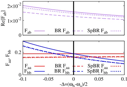
order in the damping rate, the SpBR equation is cor-rect to higher order. This suggests that as the damping rate becomes larger, the SpBR may give a better numeri-cal agreement with the exact solution. This is indeed the case, and is shown in Fig. 3 where we compare the steady state values of Fij. Comparing the coherence Fab(t), it is clear the SpBR matches the exact solution better than the BR approach. The lower panel shows that the two theories give very similar results for the populations. For the parameters corresponding to Fig. 2 the BR and SpBR lines would be indistinguishable.

Note that at ∆ = 0, the SpBR and BR formalisms are identical, and so one might expect the results to match at this point. However, the matrixMis singular at ∆ = 0 (as seen earlier from its eigenvalues). As such, the finite population and coherence at ∆→0 correspond to a singular limit.

0

1×₁₀-2

2×₁₀-2

Re[F

ab

]

F_ab BR F_ab SpBR F_ab

0 0.2

-0.1 -0.05 0 0.05 0.1

Faa

, F

bb

-∆₌₍ω

b-ωa)/2

F_aa

F_bb

BR F_aa

BR F_bb

SpBR F_aa

SpBR F_bb

FIG. 3. (Color online) Comparison of steady state values of

Fij between the exact (solid), BR master equation (dashed)

and SpBR master equation (dotted), plotted for a larger bath density of states J0 = 0.02 and all other parameters as for Fig. 2.

VI. EXTENSION TO MULTIPLE BATHS

Extending either the exact solution or the BR mas-ter equation to multiple baths is simple. For the BR master equation, one just finds a separate set of Lamb-shift terms hij and dissipator terms Lσ_ij for each bath, so that Eq. (10) involves a summation over contribu-tions from the baths. Similarly, the expressions for the matrix M follow as before, but now with a sum over baths, and even the analytic form of the eigenvalues re-mains true, with ˜Ki 7→ PnK˜

(n)

i in Eq. (14). The

ex-act solution is however more complicated. Equation (2) still holds, however there is a sum over baths, and each term now acquires a bath label: J(ν), nB(ν), W_i(ν, t)7→

J(n)_{(ν), n}(n)

B (ν), W

(n)

i (ν, t). The last of these quantities

now has a more complicated form

W_i(n)(ν, t) = Z _dζ

2π

X

j

Gij(ν)ϕ

(n)

j (23)

where the matrixGcan be defined in terms of its inverse, [G(ν)−1]ij=iδij(ωi−ν−i0) +Pnϕ

(n)∗

i ϕ

(n)

j K

(n)∗_(ν). In the presence of multiple baths, the singular behavior atωa=ωbno longer occurs — one may check this by cal-culating the zeros of Det[G(ν)−1_{]: one now finds there is} no longer a zero mode, unless the coefficientsϕ(_in)happen to be parallel for differentn. The physical origin of this is that with multiple linearly independent baths there is no longer a linear combination of fields ˆψi which decouples from the baths, and so all modes are damped. As such, the collective dephasing model is never correct for pre-dicting the steady state coherence. The non-secularized BR approach continues to correctly describe the system as one varies detuning.

VII. CONCLUSIONS

In conclusion we have compared the exact and Bloch-Redfield solutions for a system of two bosonic modes cou-pled to a common bath. The late-time behaviors show singular dependence on detuning: exactly on resonance, significant coherence exists at late times, but for arbi-trarily small detuning the coherence drops to a smaller value which depends on the frequency dependence of the density of states. This singular limit appears only at late times, corresponding to a slow decay rate for coherence that vanishes at the degenerate point. All aspects of this behavior are reproduced correctly by a non-secularized Bloch-Redfield theory, whereas secularization leads to incorrect predictions. The Bloch-Redfield theory does not guarantee positivity, nonetheless one can prove that the equations describe bounded dynamics of physical ob-servables, as long as the Markov approximation remains valid. A modification to the Bloch-Redfield theory — as-suming it is the Schr¨odinger picture density matrix that evolves slowly, rather than the interaction picture one — leads to an improved time-local theory which satisfies required sum rules and exactly matches damping rates near resonance.

ACKNOWLEDGMENTS

(RPG-080), and the joint EPSRC (EP/I035536) / NSF (DMR-1107606) Materials World Network grant.

[1] N. G. van Kampen,Stochastic Processes in Physics and Chemistry, 3rd ed. (North Holland, 2007).

[2] H.-P. Breuer and F. Petruccione, The Theory of Open Quantum Systems (Oxford University Press, Oxford, 2002).

[3] A. Badolato, K. Hennessy, M. Atat¨ure, J. Dreiser, E. Hu, P. M. Petroff, and A. Imamoglu, Science 308, 1158 (2005).

[4] A. J. Ramsay, T. M. Godden, S. J. Boyle, E. M. Gauger, A. Nazir, B. W. Lovett, A. M. Fox, and M. S. Skolnick, Phys. Rev. Lett.105, 177402 (2010).

[5] F. Nissen, J. M. Fink, J. A. Mlynek, A. Wallraff, and J. Keeling, Phys. Rev. Lett.110, 203602 (2013). [6] L. Henriet, Z. Ristivojevic, P. P. Orth, and K. Le Hur,

Phys. Rev. A90, 023820 (2014).

[7] P. Kaer, T. R. Nielsen, P. Lodahl, A.-P. Jauho, and J. Mørk, Phys. Rev. Lett.104, 157401 (2010).

[8] C. Roy and S. Hughes, Phys. Rev. Lett. 106, 247403 (2011).

[9] H. Kim, T. C. Shen, K. Roy-Choudhury, G. S. Solomon, and E. Waks, Phys. Rev. Lett.113, 027403 (2014). [10] A. Nysteen, P. Kaer, and J. Mørk, Phys. Rev. Lett.110,

087401 (2013).

[11] T. Yuge, K. Kamide, M. Yamaguchi, and T. Ogawa, J. Phys. Soc. Jpn.83, 123001 (2014).

[12] S. Diehl, A. Micheli, A. Kantian, B. Kraus, H. P. B¨uchler, and P. Zoller, Nat. Phys.4, 878 (2008).

[13] J. Paavola and S. Maniscalco, Phys. Rev. A82, 012114 (2010).

[14] T. V. Tscherbul and P. Brumer, Phys. Rev. Lett. 113, 113601 (2014).

[15] J. P. Paz and A. J. Roncaglia, Phys. Rev. Lett. 100, 220401 (2008).

[16] F. Benatti, R. Floreanini, and M. Piani, Phys. Rev. Lett. 91, 070402 (2003).

[17] D. P. S. McCutcheon, A. Nazir, S. Bose, and A. J. Fisher, Phys. Rev. A80, 022337 (2009).

[18] F. Galve, L. A. Pach´on, and D. Zueco, Phys. Rev. Lett. 105, 180501 (2010).

[19] A. F. Estrada and L. A. Pach´on, New J. Phys.17, 033038 (2015).

[20] P. R. Eastham, A. O. Spracklen, and J. Keeling, Phys. Rev. B87, 195306 (2013).

[21] C. Roy and S. Hughes, Phys. Rev. X1, 021009 (2011). [22] F. Benatti and R. Floreanini, Int. J. Mod. Phys. B19,

3063 (2005).

[23] R. D¨umcke and H. Spohn, Z. Phys. B34, 419 (1979). [24] C. Joshi, P. ¨Ohberg, J. D. Cresser, and E. Andersson,

Phys. Rev. A90, 063815 (2014).

[25] D. A. Steck, Lecture notes “Quantum and atom optics” (unpublished) .

[26] F. Benatti, R. Floreanini, and U. Marzolino, EPL88, 20011 (2009).

[27] R. Wangsness and F. Bloch, Phys. Rev.89, 728 (1953). [28] A. G. Redfield, IBM J. Res. Dev.1, 19 (1957).

[29] F. Bloch, Phys. Rev.105, 1206 (1957).

[30] G. Lindblad, Commun. Math. Phys.48, 119 (1976). [31] A. K. Rivas, A. D. K. Plato, S. F. Huelga, and M. B.

Plenio, New J. Phys.12, 113032 (2010).

[32] J. Jeske, D. Ing, M. B. Plenio, S. F. Huelga, and J. H. Cole, J. Chem. Phys142, 064104 (2015).

[33] R. S. Whitney, J. Phys. A Math. Theor. 41, 175304 (2008).

[34] S. Maniscalco, Phys. Rev. A75, 062103 (2007). [35] S. Nakajima, Progr. Theor. Phys.20, 948 (1958). [36] R. Zwanzig, J. Chem. Phys.33, 1338 (1960).

[37] M. Hell, M. R. Wegewijs, and D. P. DiVincenzo, Phys. Rev. B89, 195405 (2014).

[38] J. Salmilehto, P. Solinas, and M. M¨ott¨onen, Phys. Rev. A85, 032110 (2012).

[39] C. Karlewski and M. Marthaler, Phys. Rev. B.90, 104302 (2014).

[40] I. L. Aleiner, B. L. Altshuler, and Y. G. Rubo, Phys. Rev. B85, 121301 (2012).

[41] S. M. Barnett, J. D. Cresser, and S. Croke, arXiv:1508.02442.

[42] H. Grabert, P. Schramm, and G.-L. Ingold, Phys. Rep. 168, 115 (1988).

[43] C.-H. Chou, T. Yu, and B. L. Hu, Phys. Rev. E 77, 011112 (2008).

[44] T. M. Stace, A. C. Doherty, and D. J. Reilly, Phys. Rev. Lett.111, 180602 (2013).