Similarity based non singleton fuzzy logic control for improved performance in UAVs

Novel, Similarity-based Non-Singleton Fuzzy Logic

Control for Improved Uncertainty Handling in

Quadrotor UAVs

Changhong Fu

, Andriy Sarabakha

,

Erdal Kayacan

a_{School of Mechanical and Aerospace Engineering,} b_{ST Engineering-NTU Corp Laboratory,}

Nanyang Technological University (NTU), 50 Nanyang Avenue, Singapore, 639798.

Email: [email protected], [email protected], [email protected]

Christian Wagner

, Robert John

and Jonathan M. Garibaldi

Michigan Technological University, Houghton, Michigan, USA.

d_{Lab for Uncertainty in Data and Decision Making (LUCID),}

School of Computer Science,

University of Nottingham, Nottingham, United Kingdom. Email:{christian.wagner, robert.john, jon.garibaldi}@nottingham.ac.uk

Abstract—As non-singleton fuzzy logic controllers (NSFLCs) are capable of capturing input uncertainties, they have been effectively used to control and navigate unmanned aerial vehicles (UAVs) recently. To further enhance the capability to handle the input uncertainty for the UAV applications, a novel NSFLC with the recently introduced similarity-based inference engine, i.e., Sim-NSFLC, is developed. In this paper, a comparative study in a 3D trajectory tracking application has been carried out using the aforementioned Sim-NSFLC and the NSFLCs with the standard as well as centroid composition-based inference engines, i.e., Sta-NSFLC and Cen-NSFLC. All the NSFLCs are developed within the robot operating system (ROS) using the C++ programming language. Extensive ROS Gazebo simulation-based experiments show that the Sim-NSFLCs can achieve better control performance for the UAVs in comparison with the Sta-NSFLCs and Cen-Sta-NSFLCs under different input noise levels.

I. INTRODUCTION

Nowadays, unmanned aerial vehicles (UAVs) are widely used for various civilian and commercial applications, e.g., midair monitoring [1], vessel traffic management [2], anti-poaching patrol [3] and emergency evacuation planning [4]. In most of these applications, classical control approaches, e.g. proportional-integral-derivative control [5], sliding mode con-trol [6] and model predictive concon-trol [7], have been employed for UAVs to conduct autonomous flights. However, these well-known controllers require a precise dynamic model of the UAV and work under the assumption that significant internal as well as external uncertainties do not substantially affect the UAV systems. Achieving an accurate mathematical model for such complex aerial vehicles is often time-consuming and tedious [8]. In addition, the frequently-used sensors onboard the UAVs, e.g., global positioning system (GPS), inertial measurement unit (IMU) and camera, often lack precise modeling. Their measurements consist of numbers of uncertain, incomplete and possibly inaccurate information [9]. Further, the process of conducting a UAV application also contains numerous uncertain and challenging factors [10].

In the literature, fuzzy logic controllers (FLCs) are exten-sively used for the control and navigation of the UAVs. They are able to deliver adequate control and handle uncertainties without the requirement of an accurate mathematical UAV model. Among the different types of FLCs, singleton FLCs (SFLCs) are the most common FLCs used for the UAVs [11]. However, SFLCs are not capable of capturing input uncertain-ties effectively. Therefore, non-singleton FLCs (NSFLCs) are preferred as they can deal with the uncertainties by modeling the inputs as input fuzzy sets (FSs) [12]. In our previous paper [13], we investigated that applying two NSFLCs with standard and a novel centroid-based inference engines, i.e., Sta-NSFLC [12] and Cen-NSFLC [14], to control and stabilize the UAVs. The UAV flight results show that the Cen-NSFLCs can achieve better control performance than the Sta-NSFLCs. Furthermore, both the Sta-NSFLCs and Cen-NSFLCs outperform SFLCs under different levels of noise conditions. Despite that the NSFLCs are superior to the SFLCs, the NSFLCs applied for the UAV applications are still rare in comparison to the SFLCs. In this work, a novel NSFLC with the similarity-based inference engine, i.e., Sim-NSFLC, is developed based on our recently introduced similarity-based non-singleton fuzzy logic system (NSFLS) inference engine [15] to navigate and guide a quadrotor UAV in a 3D trajectory tracking application. In this new approach, the firing strength of each rule is calculated by the similarity between the input and antecedent FSs instead of being calculated by the standard or centroid-based approach. The similarity-based inference engine is able to make the NSFLCs more sensitive to the changes of the input uncertainty. In [15], the Sim-NSFLS showed promising results in the well-known problem of Mackey-Glass time series predictions, i.e., the Sim-NSFLS outperformed the Sta-NSFLS and Cen-NSFLS under various noise conditions.

en-able future, real-world experiments. The control performances of these NSFLCs are tested and evaluated in the ROS Gazebo environment [17], which provides a seamless connection for the developed algorithms between the simulation and real-world applications.

To the best of our knowledge, this is the first time in the literature that the similarity-based NSFLS inference is applied for control, i.e., as a Sim-NSFLC. The rest of this paper is structured as follows: Section II introduces the quadrotor UAV dynamic model and control structure. Section III presents a brief background for the NSFLCs. Section IV evaluates the control performances with all three NSFLCs under different input noise levels. Finally, Section V presents the conclusions and future work.

II. QUADROTORUAV DYNAMICS ANDCONTROL STRUCTURE

A. Quadrotor UAV Dynamics

In this work, the Parrot ARDrone 2 quadrotor UAV [18], as its Gazebo model shown in Fig. 1, is used to test and evaluate the NSFLCs. Let the world inertial reference frame beFI, i.e.,

{~xI, ~yI, ~zI}, and the body frame be FB, i.e., {~xB, ~yB, ~zB}.

Figure 1 illustrates the quadrotor UAV configuration and reference frames.

To achieve the translations and rotations of the quadrotor UAV, the thrust of four rotors fi, i = 1, . . . ,4, are adjusted

with various combinations. The thrust from each rotor is changed by controlling the angular speed wi, i = 1, . . . ,4

of the motors. The control input vector c of quadrotor UAV is represented as:

c=T τφ τθ τψ T

, (1) where T is the total thrust along the ~zB axis; and τφ, τθ

and τψ are the moments acting on the ~xB,~yB and~zB axes,

respectively. Then, the relationship between the control input cand angular speedωi,i= 1, . . . ,4, is as follows [19]:

        

T =b ω2

1+ω22+ω23+ω24

τφ = √

2 2 bl ω

2

1+ω22−ω32−ω24

τθ = √

2 2 bl −ω

2

1+ω22−ω23+ω42

τψ =d −ω12+ω 2 2+ω

2 3−ω

2 4 , (2) 𝑇 𝑓1 𝑓4 𝑓3 𝑓2

𝑥 𝐵

𝑦 𝐵

𝑧 𝐵

𝜔1

𝜔2

𝜔4

𝜔3

𝑥 𝐼

𝑦 𝐼

𝑧 𝐼

ℱ𝐼

ℱ𝐵

Fig. 1: Quadrotor UAV model with reference frames.

wherebis the coefficient of propeller thrust,dis the coefficient of propeller drag andl is the quadrotor UAV arm length.

Let the absolute position of the quadrotor UAV be the three Cartesian coordinates of its mass center in the world frameFI,

i.e,p=

x y zT

, and its attitude be the three Euler angles, i.e,o=φ θ ψT

, called roll, pitch and yaw, respectively. The time derivative of the absolute position is denoted asv=

˙

x y˙ z˙T

=

u v wT

,wherevis the absolute velocity of the quadrotor UAV’s mass center inFI. Moreover, the time

derivative of the attitude is ω = _˙

φ θ˙ ψ˙T

, which is the angular velocity inFI, and the angular velocity inFBisωB =

p q rT

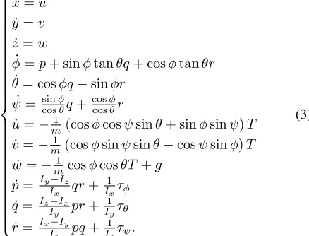
. The dynamical model of the quadrotor UAV is [20]:                                                  ˙

x=u

˙

y=v

˙

z=w

˙

φ=p+ sinφtanθq+ cosφtanθr

˙

θ= cosφq−sinφr

˙

ψ=sin_cosφ_θq+cos_cosφ_θr

˙

u=−1

m(cosφcosψsinθ+ sinφsinψ)T ˙

v=−1

m(cosφsinψsinθ−cosψsinφ)T ˙

w=−1

mcosφcosθT +g ˙

p= Iy−Iz Ix qr+

1 Ixτφ ˙

q=Iz−Ix Iy pr+

1 Iyτθ ˙

r=Ix−Iy Iz pq+

1 Izτψ.

(3)

wherem is the mass of the quadrotor UAV, g is the gravity acceleration, i.e,g= 9.81m/s2, andI=diag(Ix, Iy, Iz)is the

inertia matrix. As can be seen from the above dynamic equa-tions, these equations are coupled, non-linear and the system to be controlled is underactuated. Additionally, as discussed uncertainties in the real-world control of the quadrotor UAV are inevitable. Hence, a fuzzy logic controller is utilized in this work instead of using a model-based linear controller.

B. Control Structure

The high-level NSFLC-based closed-loop control struc-ture is illustrated in Fig. 2. It consists of two modules (shown with dashed rectangles): the position controller and the quadrotor UAV. The position controller module includes three independent NSFLCs, which take the desired position pd =

xd yd zd T

and current measured position p =

x y zT

as the inputs, and then compute the control commandud, i.e., the desired rollφd, desired pitchθd angles

and desired vertical velocity vz

d. Specifically, considering the

x-axis NSFLC as an example, the errorex, i.e.,xd−x, the

integral of the errorR ex and the derivative of the error dex

are calculated, and then thex-axis NSFLC outputs the desired roll φd. The detail on how the NSFLC converts these errors

Quadrotor UAV Position controller

NSFLC_y

NSFLC_x

NSFLC_z

Velocity/Attitude Controller

Sensors: Camera, IMU, GPS, etc 𝜃𝑑

𝑣_𝑑𝑧 𝜙_𝑑

𝐩_𝑑

𝐮_𝑑

𝐩

𝑥𝑑

𝑦𝑑

𝑧𝑑

𝑥

𝑦

𝑧

Fig. 2: The NSFLC-based closed-loop control structure for the navigation of the quadrotor UAV.

current position of the quadrotor UAV and thus the input to the FLC, see [9].

III. BACKGROUND OFNSFLCS

A. Structure of NSFLC

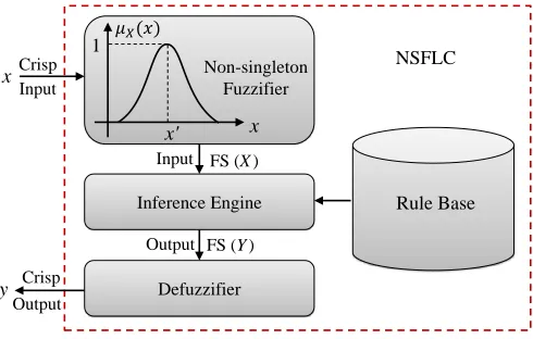
Figure 3 shows the general structure of a NSFLC, which includes fuzzifier, inference engine, rule base and defuzzifier. Specifically, the NSFLC utilizes a non-singleton fuzzifier to model the input uncertainties. In other words, the fuzzifier maps a crisp input to an input FS with a membership function (MF) aroundx0 for handling the uncertainties from the actual input. In this work, a Gaussian distribution is employed for the fuzzifier:

µX(xi) = exp

−(xi−x0i) 2

2σ2 F

. (4) wherex0_iis the input crisp value and the mean value of the FS.

σF is the spread of the FS. Larger values of theσF imply that

more noise is expected in relation to the input data. It is noted that the crisp input can be a vector with multiple elements, as the three inputs ex,

R

ex and dex. And each element in this

vector is fuzzified with a Gaussian distribution.

In the literature, NSFLCs which have been used for con-trolling UAVs, can be generally divided into two types based

Inference Engine Crisp

Crisp x

y

Input

NSFLC Non-singleton

Fuzzifier 1

x' x

FS (X)

Output FS (Y)

Output Input

ߤ𝑋(𝑥)

Defuzzifier

Rule Base

Fig. 3: General structure of a NSFLC.

on different composition-based inference engines [13]: (I) the NSFLC with standard composition-based inference engine [12], i.e., Sta-NSFLC and (II) the NSFLC with centroid composition-based inference engine [14], i.e., Cen-NSFLC. In the Cen-NSFLC, the centroid of the FS intersection between the input and antecedent FSs is used for calculating the firing strength of each rule rather than the maximum of the intersection utilized in Sta-NSFLCs. The main motivation in this paper is to leverage an even more effective mechanism to integrate the input uncertainty into the inference engine, thereby making the NSFLCs more sensitive to the changes of the input uncertainty model in comparison with the Sta-NSFLC and Cen-Sta-NSFLC. Then next subsections introduce the Sta-NSFLC, the recently introduced improved Cen-NSFLC and the novel Sim-NSFLC.

B. The standard NSFLC Inference Engine for UAV control

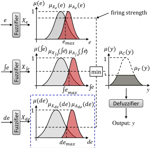
The general mapping between the inputs and outputs of the NSFLC, i.e, the input set X and output set Y shown in Fig. 3, is described in Fig. 4. To keep the description con-sistent with Section II-B, we still consider thex-axis NSFLC as an example. A triple-input, single-rule and single-output discrete NSFLC is considered, and the Mamdani implication is employed. Figure 4 illustrates the calculation from inputs (Xe, Xde and XR

e), antecedents (Ae, Ade and AR

e) and

consequent (C) fuzzy sets to output (Y) of a Sta-NSFLC. Here, the crisp input is a vector which includes three elements, i.e., x = e de R

eT

, as discussed in the Section II-B. The e, de and Re are the members of the input FSs Xe,

Xde and XR

e, respectively. y is the member of the output

FS (Y). Moreover, µX∗(∗), µA∗(∗), µC(y) and µY(y) be

the membership functions (MFs) of X∗, A∗, C and Y,

respectively. The defined rule is as follows:

IFeisAeANDdeisAdeAND Z

eisAR

e THENy isC.

(5) The input-output mapping of the Sta-NSFLC is:

µY(y) = min[µC(y), min[µe, µde, µR

e 𝜇(𝑒) _𝜇

𝑋𝑒(𝑒)

𝑒𝑚𝑎𝑥

1

𝜇𝐴𝑒(𝑒)

de 𝜇(𝑑𝑒)

𝜇𝑋𝑑𝑒(𝑑𝑒)

𝑑𝑒𝑚𝑎𝑥

1

𝜇𝐴𝑑𝑒(𝑑𝑒) ∫ 𝜇(∫ )_𝜇

𝑋_∫(∫ )

∫_𝑚𝑎𝑥 1

𝜇𝐴_∫(∫ )

𝑒 _{𝑒 𝑒}

𝑒 𝑒

𝑒 𝑒

1

min 𝜇(𝑦) _𝜇

𝐶(𝑦)

y 𝜇𝑌 (𝑦)

Output: y Defuzzifier firing strength

Fuzzif

ier

Fuzzif

ier

Fuzzif

ier

𝑒

𝑑𝑒 ∫𝑒

𝑋𝑒

𝑋𝑑𝑒

𝑋_∫𝑒

Fig. 4: Example of the calculation from inputs (X∗),

an-tecedents (A∗) and consequent (C) fuzzy sets to output (Y)

of a Sta-NSFLC.

where,

µe= max[µXe(e)? µAe(e)],

µR

e= max[µXR e(

Z

e)? µAR e(

Z

e)], µde= max[µXde(de)? µAde(de)].

whereµX∗(∗)? µA∗(∗) is the intersection ofX∗ andA∗.

The above equations show that the firing level of an an-tecedent is the maximum of its intersection with the input FS.

C. The NSFLC with Centroid-based Inference Engine (Cen-NSFLC)

To make the NSFLC more sensitive to the input uncertainty, the Cen-NSFLCs have been presented to control and stabilize the UAVs recently [13]. Taking the derivative of errorde for example (as the blue rectangle shown in the Fig. 4), two different input FSs, i.e. X1

de andXde2, which are intersected

with the same antecedent Ade, are considered, as shown in

Fig. 5. Despite that the actual input FSs are different, the firing levels calculated by the standard approach in the Sta-Com-NSFLC are the same in both cases, i.e.,µ1_X

de(demax) =

µ2_X

de(demax) =α. While the centroid-based approach in the

Cen-Com-NSFLC has higher sensitivity to the shape of the intersection between the input FS and antecedent FS, i.e., these two various inputs with a different associated uncertainty distribution can generate two different firing levels, i.e.,βand

γ.

1

de 𝜇(𝑑𝑒)

𝜇𝑋𝑑𝑒(𝑑𝑒)

𝑑𝑒_𝑚𝑎𝑥

𝜇𝐴𝑑𝑒(𝑑𝑒) 𝜇𝑋𝑑𝑒2 (𝑑𝑒)

1

𝑑𝑒𝑐𝑒𝑛1

𝑑𝑒𝑐𝑒𝑛2

α β

γ

Fig. 5: The difference between the Cen-NSFLC and Sta-NSFLC.α,β andγ are the different firing levels.

Considering a discrete FSXdewith a membership function

µXde(dei), the centroid of Xde is defined as:

xcen(Xde) = Pn

i=1deiµXde(dei)

Pn

i=1µXde(dei)

, (7) wherenis the number of discretization levels (we setn=100 for our work) utilized in a discrete system.

The input-output mapping of the Cen-NSFLC is:

µY(y) = min[µC(y), min[µe, µde, µR

e]], (8)

where,

µe=µXe∩Ae(xcen(Xe∩Ae)),

µR_e=µ_XR e∩AR

e(xcen(XRe∩ARe)),

µde=µXde∩Ade(xcen(Xde∩Ade)).

xcen(X∗∩A∗)is the centroid of the intersection of an input

X∗ and an antecedent A∗. The aforementioned formulations

show that the firing level of an antecedent is its membership degree at the centroid of the intersection with the input FS.

Although the Cen-NSFLC outperformed the Sta-NSFLC for the autonomous control and stabilization of the UAVs in our previous work [13]. Based on [15], we hypothesize that the performance of the NSFLCs can be further improved in our UAV tests by replacing the composition-based inference engine with the similarity-based inference engine as outlined next.

D. The Similarity-based NSFLC (Sim-NSFLC)

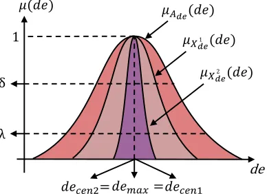
We start by illustrating the rationale for the Sim-NSFLS as originally outlined in [15]. Figure 6 shows intersections of two different input FSs with one antecedent FS, although these two different input FSs have two different associ-ated uncertainty distributions. The standard and centroid-based firing strengths of Ade for both Xde1 and X

2

de are the

same, i.e, µ1

Xde(decen1) = µ 2

Xde(decen2) = µ 1

Xde(demax) =

µ2

Xde(demax) = 1. Hence, a new NSFLS, which is more

1

de

𝑑𝑒_𝑚𝑎𝑥=

𝜇𝐴𝑑𝑒(𝑑𝑒)

𝜇𝑋𝑑𝑒2 (𝑑𝑒) 𝜇𝑋𝑑𝑒1 (𝑑𝑒)

𝑑𝑒𝑐𝑒𝑛1

𝑑𝑒𝑐𝑒𝑛2=

δ

λ

Fig. 6: The difference for the Sim-NSFLC, Cen-NSFLC and Sta-NSFLC. δ andλare the different firing strengths ofAde

for X1

de andXde2.

engine, i.e., Sim-NSFLS, was presented and used for the well-known problem of Mackey-Glass time series predictions. The prediction results showed that the Sim-NSFLS outperformed the Sta-NSFLS and Cen-NSFLS under different noise condi-tions.

As shown in the Fig. 6, δ and λ are two different firing levels for two different inputs based on the similarity-based approach. In this work, the Sim-NSFLC is developed to control and navigate the UAVs in a 3D trajectory tracking application. Considering the input FSXdeand antecedent FS Adewith

membership functions µXde(de)andµAde(de), the similarity

between the Xde and Ade is defined based on the Jaccard

similarity [21]:

s(Xde, Ade) = R

de∈Xdemin(µXde(de), µAde(de))

R

de∈Xdemax(µXde(de), µAde(de))

, (9)

In a discrete domain, the above equation can be rewritten as:

s(Xde, Ade) = Pn

i=1min(µXde(de), µAde(de))

Pn

i=1max(µXde(de), µAde(de))

, (10) where n is also the number of discretization levels (we set

n=100 for our work).

The input-output mapping of the Sim-NSFLC is:

µY(y) = min[µC(y), min[µe, µde, µR

e]], (11)

where,

µe=s(Xe, Ae),

µR

e=s(XR

e, AR

e),

µde=s(Xde, Ade).

The above formulations show that the firing level is the similarity between the antecedent and the input FS. The fol-lowing section investigates the control performance of the Sim-NSFLC and compare it with the composition-based Sim-NSFLCs, i.e., Sta-NSFLC and Cen-NSFLC.

IV. SIMULATIONSTUDIES

In this section, extensive quadrotor UAV simulation tests are presented for all three types of NSFLC. Below, we commence by detailing the experimental setup in Sections IV-A to IV-D before reviewing the results in Section IV-F.

A. 3D trajectory generation

The 3D trajectory is defined according to the minimize snap property [22], which enables the real-time generation of an optimal trajectory through a sequence of 3D positions, thereby ensuring safe passage through specified environments as well as maintaining the constraints on accelerations and velocities. Some manoeuvrable flights were generated, e.g., descending and climbing straight lines as well as curves, the sharp turns between the straight lines and curves, to test the control performance of each NSFLC controller. It is noted that the generated 3D trajectory is sent to all the NSFLCs at the same time.

B. Fuzzifier, Membership Function and Rule Base

In this work, different Gaussian MFs (with different stan-dard deviations) are tested to evaluate the capture capability for the expected input uncertainty or noise in each of the NSFLC controllers. Specifically, each input variable, i.e., error, the integral of the error or the derivative of the error, has three MFs, and the output variable has five MFs. Table I shows the rule base of each NSFLC, where each abbreviation Z, N, P, S, B represents zero, negative, positive, small or big, respectively.

C. Intrinsic parameters of quadrotor UAV

Table II shows the intrinsic parameters of quadrotor UAV. These intrinsic parameters are determined based on the ones of a real Parrot AR Drone 2 quadrotor UAV.

TABLE I: Rule Base for all NSFLCs Integral

Error

Derivative Error

Proportional Error

N Z P

N

N BP BP SP

Z BP SP Z

P SP Z SN

Z

N BP SP Z

Z SP Z SN

P Z SN BN

P

N SP Z SN

Z Z SN BN

P SN BN BN

TABLE II: The intrinsic parameters of quadrotor UAV. Parameter Value Unit

b 8.54×10−6 _[N·s2_]

d 1.6×10−2 [N·m·s2_]

Ix 0.007 [kg·m2]

Iy 0.007 [kg·m2]

Iz 0.012 [kg·m2]

l 0.18 [m]

D. Noise generation

In our work, the Gaussian noise is defined by a noise generator, which injects the noise to the sensors of each UAV at the same time. The noise level is parameterized by its standard deviation σN. It can be converted to SNR, which

is also commonly used to define the noise, i.e,: SNR = 10 log_10σ12

N

. Therefore, the noisy position measurement ¯

p=x¯ y¯ z¯T is defined as: ¯

x=N(x, σ_N2), (12) ¯

y=N(y, σ_N2), (13) ¯

z=N(z, σN2). (14)

whereN(µ, σ2)is the Gaussian distribution with meanµand variance σ2.

E. Control Performance Evaluation

The control performance evaluation is conducted in terms of the mean squared error (MSE) of the 3D position, epos:

epos= 1

n

n X

k=1

p

(x(k)−x∗₎2_{+ (y(k)−y}∗₎2_{+ (z(k)−z}∗₎2_,

(15)

wherex(k),y(k)andz(k)are the translations alongx-,y- and

z-axis, andx∗,y∗ andz∗ represent the desired 3D position.

F. Simulation Results

In this work, eleven levels of noise and five instances of the NSFLCs with different input fuzzifications (i.e., different standard deviations for input MFs) are provided to test and evaluate the quadrotor UAV control performances using the aforementioned three NSFLCs. Each combination of the noise and fuzzifer for one NSFLC is evaluated for 30 times. Figure 7 shows the example of three UAV flights with the same level of fuzzifier (σF=1.0) under three different levels of

noise (σN=0.0, 0.5 and 1.0). Table III shows the average

MSE of the 3D position. As can be seen from Table III, the Cen-NSFLCs outperform the Sta-NSFLCs, and the control performances of the Sim-NSFLCs are better than both the Cen-NSFLCs and Sta-Cen-NSFLCs. In addition, the larger values of theσF for the fuzzifier can assist the NSFLCS to achieve the

better performances. Figure 8 also clearly shows the control performance differences among the Sta-NSFLC, Cen-NSFLC and Sim-NSFLC.

A demonstration video related to our work can be found at: https://youtu.be/NVfgz38RFuA.

-2

x [m]

2 2 0 -2

y [m]

3

2

1

0

z

[m

]

Ref. trajectory Sta-NSFLC Cen-NSFLC Sim-NSFLC

(a)σF=1.0,σN=0.0

-2

x [m]

2 2 0

y [m]

-2 3

0 1 2

z

[m

]

Ref. trajectory Sta-NSFLC Cen-NSFLC Sim-NSFLC

(b)σF=1.0,σN=0.5

-2

x [m]

2 2 0

y [m]

-2 3

2

1

0

z

[m

]

Ref. trajectory Sta-NSFLC Cen-NSFLC Sim-NSFLC

(c)σF=1.0,σN=1.0

Fig. 7: Example of three UAV flights with the same input fuzzification (σF=1.0) under three different levels of noise.

TABLE III: Average MSE of 3D Position (Unit: Meter)

NSFLC / Noise Level (σN) 0.0 0.1 0.2 0.3 0.4 0.5 0.6 0.7 0.8 0.9 1.0

Sta-NSFLC (σF=0.2) 0.0202 0.0267 0.0643 0.1065 0.1514 0.2079 0.2686 0.4069 0.4674 0.4938 0.6469

Cen-NSFLC (σF=0.2) 0.0165 0.0231 0.0534 0.0969 0.1436 0.1910 0.2413 0.3781 0.3929 0.4657 0.5646

Sim-NSFLC (σF=0.2) 0.0136 0.0222 0.0487 0.0866 0.1398 0.1862 0.2373 0.3156 0.3407 0.4348 0.4758

Sta-NSFLC (σF=0.4) 0.0168 0.0258 0.0642 0.0921 0.1423 0.2026 0.2619 0.3738 0.4650 0.4917 0.6271

Cen-NSFLC (σF=0.4) 0.0132 0.0240 0.0603 0.0876 0.1361 0.2003 0.2608 0.3482 0.3022 0.4476 0.5190

Sim-NSFLC (σF=0.4) 0.0117 0.0229 0.0528 0.0860 0.1233 0.1729 0.2585 0.3132 0.2902 0.3806 0.4603

Sta-NSFLC (σF=0.6) 0.0121 0.0243 0.0626 0.0916 0.1412 0.1978 0.2617 0.3637 0.3843 0.4586 0.5589

Cen-NSFLC (σF=0.6) 0.0119 0.0220 0.0592 0.0911 0.1372 0.1974 0.2329 0.3309 0.3783 0.4472 0.5059

Sim-NSFLC (σF=0.6) 0.0112 0.0204 0.0502 0.0857 0.1225 0.1646 0.2241 0.2448 0.3572 0.4348 0.4478

Sta-NSFLC (σF=0.8) 0.0114 0.0267 0.0541 0.0944 0.1413 0.1615 0.2372 0.3234 0.3645 0.4581 0.4986

Cen-NSFLC (σF=0.8) 0.0118 0.0243 0.0509 0.0904 0.1368 0.1450 0.2326 0.2941 0.3302 0.3960 0.4694

Sim-NSFLC (σF=0.8) 0.0103 0.0200 0.0434 0.0785 0.1150 0.1433 0.2317 0.2802 0.3225 0.3721 0.4417

Sta-NSFLC (σF=1.0) 0.0109 0.0242 0.0472 0.0844 0.1366 0.1610 0.2361 0.3143 0.3332 0.3977 0.4160

Cen-NSFLC (σF=1.0) 0.0106 0.0211 0.0440 0.0805 0.1317 0.1405 0.2206 0.2610 0.2857 0.3543 0.3650

Noise Level

0.0 0.2 0.4 0.6 0.8 1.0

M

S

E

E

rr

or

[m

]

0 0.1 0.2 0.3 0.4 0.5 0.6 0.7

Sta-NSFLC (σ

F=0.2)

Cen-NSFLC (σ

F=0.2)

Sim-NSFLC (σ

F=0.2)

Sta-NSFLC (σ

F=1.0)

Cen-NSFLC (σ

F=1.0)

Sim-NSFLC (σ

F=1.0)

Fig. 8: Control performances of the Sta-NSFLC, Cen-NSFLC and Sim-NSFLC in 3D trajectory tracking task.

V. CONCLUSION ANDFUTUREWORK

In this work, a novel NSFLC with similarity-based in-ference engine has been developed and deployed to control simulated UAVs in the 3D trajectory tracking application. A comprehensive comparison and evaluation has been carried out with three different types of NSFLCs, i.e., Sta-NSFLC, Cen-NSFLC and the novel Cen-NSFLC (Sim-Cen-NSFLC), under different levels of input uncertainty, i.e., noise. The aim of this work was not only to evaluate the control performances among these three NSFLCs, but also to explore better NSFLCs for the real-world UAV applications. All the NSFLCs are programmed in the C++ language and evaluated in the ROS and Gazebo environment. The extensive simulation tests show that the Sim-NSFLC can obtain better control performances compared to the Sta-NSFLC and Cen-NSFLC, especially at the higher input noise levels. Moreover, the different input fuzzifications can achieve the various capabilities for capturing input uncertain-ties. In other words, the higher input fuzzification has more capability to handle higher level input noise. These results support the results in [15].

For future work, the experiments on real-world quadrotor UAVs will be conducted and we will extend this approach to different Type-2 FLCs to control the quadrotor UAVs, and compare their performances under different input noise levels. Finally, the novel NSFLC architecture provides improved capacity to explore detailed input uncertainty models (captured in the input fuzzy sets), thus a key aspect of our future work is to develop improved techniques to appropriately capture real-world input noise/uncertainty in the input MFs of the FLCs.

ACKNOWLEDGMENT

This research work was partially supported by the ST Engineering-NTU Corporate Lab through the NRF corporate lab@university scheme. This work was also partially funded by the RCUK’s EP/M02315X/1 From Human Data to Personal Experience grant.

REFERENCES

[1] C. Fu, A. Carrio, M. Olivares-Mendez, R. Suarez-Fernandez, and P. Campoy, “Robust real-time vision-based aircraft tracking from Un-manned Aerial Vehicles,” in Robotics and Automation (ICRA), IEEE International Conference on, 2014, pp. 5441–5446.

[2] M. Mueller, N. Smith, and B. Ghanem, “A Benchmark and Simulator for UAV Tracking,” in14th European Conference on Computer Vision (ECCV), 2016, pp. 445–461.

[3] M. A. Olivares-Mendez, C. Fu, P. Ludivig, T. F. Bissyande, S. Kan-nan, M. Zurad, A. Annaiyan, H. Voos, and P. Campoy, “Towards an Autonomous Vision-Based Unmanned Aerial System against Wildlife Poachers,”Sensors, vol. 15, no. 12, pp. 31 362–31 391, 2015. [4] A. Sarabakha and E. Kayacan, “Y6 tricopter autonomous evacuation in

an indoor environment using q-learning algorithm,” in2016 IEEE 55th Conference on Decision and Control (CDC), 2016, pp. 5992–5997. [5] J. Pestana, I. Mellado-Bataller, C. Fu, J. L. Sanchez-Lopez, I. F.

Mondragon, and P. Campoy, “A general purpose configurable navigation controller for micro aerial multirotor vehicles,” inInternational Confer-ence on Unmanned Aircraft Systems (ICUAS), 2013, pp. 557–564. [6] J. R. Hervas, E. Kayacan, M. Reyhanoglu, and H. Tang, “Sliding mode

control of fixed-wing uavs in windy environments,” in13th International Conference on Control Automation Robotics Vision (ICARCV), 2014, pp. 986–991.

[7] K. Alexis, C. Papachristos, R. Siegwart, and A. Tzes, “Robust Model Predictive Flight Control of Unmanned Rotorcrafts,”Journal of Intelli-gent & Robotic Systems, vol. 81, no. 3, pp. 443–469, 2016.

[8] T. Lee, M. Leok, and N. H. McClamroch, “Nonlinear Robust Tracking Control of a Quadrotor UAV on SE(3),” Asian Journal of Control, vol. 15, no. 2, pp. 391–408, 2013.

[9] C. Fu, A. Carrio, and P. Campoy, “Efficient visual odometry and mapping for Unmanned Aerial Vehicle using ARM-based stereo vision pre-processing system,” inUnmanned Aircraft Systems (ICUAS), Inter-national Conference on, 2015, pp. 957–962.

[10] K. S. Pratt, R. Murphy, S. Stover, and C. Griffin, “CONOPS and autonomy recommendations for VTOL small unmanned aerial system based on Hurricane Katrina operations,” Journal of Field Robotics, vol. 26, no. 8, pp. 636–650, 2009.

[11] C. Fu, M. A. Olivares-Mendez, R. Suarez-Fernandez, and P. Campoy, “Monocular Visual-Inertial SLAM-Based Collision Avoidance Strategy for Fail-Safe UAV Using Fuzzy Logic Controllers,”Journal of Intelligent & Robotic Systems, vol. 73, no. 1, pp. 513–533, 2014.

[12] J. Mendel,Uncertain rule-based fuzzy logic system: introduction and new directions. Upper Saddle River, NJ, USA, Prentice-Hall, 2001. [13] C. Fu, A. Sarabakha, E. Kayacan, C. Wagner, R. John, and J. M.

Garibaldi, “A comparative study on the control of quadcopter uavs by using singleton and non-singleton fuzzy logic controllers,” inIEEE International Conference on Fuzzy Systems (FUZZ-IEEE), 2016, pp. 1023–1030.

[14] A. Pourabdollah, C. Wagner, J. H. Aladi, and J. M. Garibaldi, “Improved uncertainty capture for nonsingleton fuzzy systems,”IEEE Transactions on Fuzzy Systems, vol. 24, no. 6, pp. 1513–1524, 2016.

[15] C. Wagner, A. Pourabdollah, J. McCulloch, R. John, and J. M. Garibaldi, “A similarity-based inference engine for non-singleton fuzzy logic systems,” inIEEE International Conference on Fuzzy Systems (FUZZ-IEEE), 2016, pp. 316–323.

[16] “Robot Operating System (ROS),” http://www.ros.org/, 2016. [17] “Gazebo,” http://www.gazebosim.org/, 2016.

[18] “ARDrone Parrot 2,” https://www.parrot.com/, 2016.

[19] R. Mahony, V. Kumar, and P. Corke, “Multirotor Aerial Vehicles: Mod-eling, Estimation, and Control of Quadrotor,”IEEE Robotics Automation Magazine, vol. 19, no. 3, pp. 20–32, 2012.

[20] A. Sarabakha, “Reactive obstacle avoidance for quadrotor UAVs based on dynamic feedback linearization,” Master’s thesis, 2015.

[21] P. Jaccard, “Distribution de la flore alpine dans le bassin des Dranses et dans quelques regions voisines,”Bulletin de la Societe Vaudoise des Sciences Naturelles, vol. 37, pp. 241–272, 1901.