Neural field models with threshold noise

DOI 10.1186/s13408-016-0035-z

R E S E A R C H Open Access

Neural Field Models with Threshold Noise

Rüdiger Thul1·Stephen Coombes1· Carlo R. Laing2

Received: 26 November 2015 / Accepted: 19 February 2016 /

© 2016 Thul et al. This article is distributed under the terms of the Creative Commons Attribution 4.0 International License (http://creativecommons.org/licenses/by/4.0/), which permits unrestricted use, distribution, and reproduction in any medium, provided you give appropriate credit to the original author(s) and the source, provide a link to the Creative Commons license, and indicate if changes were made.

Abstract The original neural field model of Wilson and Cowan is often interpreted

as the averaged behaviour of a network of switch like neural elements with a distri-bution of switch thresholds, giving rise to the classic sigmoidal population firing-rate function so prevalent in large scale neuronal modelling. In this paper we explore the effects of such threshold noise without recourse to averaging and show that spatial correlations can have a strong effect on the behaviour of waves and patterns in con-tinuum models. Moreover, for a prescribed spatial covariance function we explore the differences in behaviour that can emerge when the underlying stationary distri-bution is changed from Gaussian to non-Gaussian. For travelling front solutions, in a system with exponentially decaying spatial interactions, we make use of an interface approach to calculate the instantaneous wave speed analytically as a series expansion in the noise strength. From this we find that, for weak noise, the spatially averaged speed depends only on the choice of covariance function and not on the shape of the stationary distribution. For a system with a Mexican-hat spatial connectivity we further find that noise can induce localised bump solutions, and using an interface stability argument show that there can be multiple stable solution branches.

Keywords Stochastic neural field·Interface dynamics·Fronts·Bumps· Non-Gaussian quenched disorder

B

[email protected]

S. Coombes

[email protected]

C.R. Laing

[email protected]

1 _{Centre for Mathematical Medicine and Biology, School of Mathematical Sciences, University of}

Nottingham, University Park, Nottingham, NG7 2RD, UK

2 _{Institute of Natural and Mathematical Sciences, Massey University (Albany), Private Bag}

1 Introduction

The study of waves, bumps and patterns in models of Wilson–Cowan type [1] is now a very mature branch of mathematical neuroscience, as discussed in the review by Bressloff [2], with many practical applications to topics including working mem-ory, visual processing, and attention. For a recent and comprehensive description of neural fields and their applications we refer the reader to the book [3]. It is only rel-atively recently that stochastic effects in neural fields have begun to be considered, with important applications to problems such as binocular rivalry waves [4] and per-ceptual switching [5]. These stochastic models are often obtained by considering the addition of noisy currents (notionally a “Gaussian random noise”) to standard (de-terministic) neural fields, and the resulting models are cast as stochastic nonlinear integro-differential equations driven by a Wiener process, such as in [6–14]. A rigor-ous probabilistic framework in which to study these equations has recently been pro-vided by Faugeras and Inglis [15]. The analysis of patterns, waves and bumps in such models has been possible utilising tools from stochastic centre manifold theory (espe-cially tools for weak noise analysis), Fokker–Planck reductions, and other techniques from stochastic calculus developed previously for PDEs. For a recent perspective on this approach the book by Bressloff is a highly valuable resource [16], as well as the paper by Inglis and MacLaurin [17], which presents a general framework in which to rigorously study the effect of spatio-temporal noise on travelling wave fronts. Indeed there is now a quite elegant body of rigorous theory growing up around neural field models with multiplicative stochastic forcing, as exemplified in the paper by Krüger and Stannat [18] using multiscale analysis, which moves beyond formal perturbation methods, to understand front propagation in particular. However, the original work of Wilson and Cowan suggests that another, perhaps more natural, way to introduce stochasticity into neural field models is by treating some of the system parameters as random variables. Indeed, threshold noise in a linear integrate-and-fire model is able to fit real firing patterns observed in the sensory periphery [19]. The simplicity of such models is also appealing from a theoretical perspective, and for a threshold described by an Ornstein–Uhlenbeck process it has recently been shown that analyt-ical (and non-perturbative) expressions for the first-passage time distribution can be obtained [20].

To appreciate the original idea of Wilson and Cowan that threshold noise in switch-ing networks can give rise to a probabilistic interpretation of network dynamics in terms of a smooth firing-rate function it is enough to consider a simple discrete time model for the evolution of neural activityxi(t ),i=1, . . . , N, in a network with con-nectionswij:

xi(t+1)=H

j

wijxj(t )−h

. (1)

take the ensemble average of the above and find

xi(t+1)=f

j

wijxj(t )

, (2)

wheref (u)=_−∞∞ H (u−h)φ (h)dh. Thus we obtain a smooth nonlinear determin-istic model describing the average behaviour of a set of switch like elements with random thresholds, with the link between the two determined by the relationship

f=φ. Sinceφis a probability distribution, this relationship immediately implies a monotonically increasing firing-rate function. Given a realisation of the thresholdshi at some timet, it is of interest to ask how the spatial covariance structure of these random thresholds affects network dynamics. This is precisely the question we wish to address in this paper for continuum models of Wilson–Cowan type, in which the random firing threshold is now described as spatially continuous quenched disorder. Although we will restrict our attention to a Gaussian covariance function, we shall consider a broad class of stationary distributions, and present practical techniques from applied mathematics and statistics for working with non-Gaussian distributions. Moreover, by working with the Heaviside choice, as in (1), we will be able to build on the interface approach of Amari [21] to obtain explicit results for travelling fronts and bumps, and their dependence on the threshold noise structure.

In Sect.2we introduce our neural field model of choice, as well as the form of the stochastic threshold, namely its steady state distribution and spatial covariance struc-ture. In Sect.3we show that, for a given realisation of the threshold, we may use the Amari interface approach to determine the instantaneous speed of a travelling front. We further show how to calculate the effects of the quenched spatial disorder arising from the noisy threshold using a perturbative approach, valid for small deviations of the threshold from its average value. We extend the approach for fronts to tackle sta-tionary bumps in Sect.4, where we also show how to determine the linear stability of localised solutions. This leads to a prediction that noise can induce multiple stable bumps, which we confirm numerically. Indeed throughout the paper we use direct numerical simulations to illustrate the accuracy of all theoretical predictions. Finally in Sect.5we discuss natural extensions of the work in this paper.

2 The Model

For mathematical convenience it is often easier to work with spatially continuous models rather than lattice models of the type described by (1). We consider a neural fieldu=u(x, t )∈R,x∈ [0, L],t∈R+, whose dynamics is given by

∂u

∂t = −u+

L

0

w|x−y|Hu(y, t )−h(y)dy. (3)

the model given by (3) is a standard Amari neural field model for the choice thath, the firing threshold, is a constant function. In this case the model is well known to support travelling waves, including fronts [22] and localised bump states in systems with a mixture of excitation and inhibition. For a review of such behaviour see [23], and for a recent overview of neural field modelling in general see [3].

In this paper we shall consider the case thathis a spatially random function. Given the wealth of mathematical knowledge for Gaussian disorder it would be highly con-venient to make this choice for the threshold. However, this is a non-physiological convenience that we would prefer to avoid. Indeed it is very natural to expect thresh-old noise to be bounded and unlikely to be best described by a symmetric distribution. As such we will consider both Gaussian and non-Gaussian disorder and in particular skewed exponential distributions and distributions with compact support. We shall explicitly model the random firing thresholdh(x)as

h(x)=h0+g(x), (4)

where h0>0 corresponds to the mean of the threshold, and g(x) denotes the quenched disorder with symmetric, bounded and non-negative spatial covariance function C(x, y). We shall fix this to be a Gaussian shape such that C(x, y)= C(|x−y|), with

C(x)=σ2exp

−πx

2

κ2

. (5)

Hereκis the correlation length of the quenched disorder. Note that the variance of the threshold is given by2σ2. There exists a sequence of non-negative real numbers,λm,

m≥1, which are eigenvalues of the covariance operator, associated with a sequence of eigenfunctions,em,m≥1, according to

L

0

C(x, y)em(y)dy=λmem(x), (6)

that form a complete orthonormal basis so that we may represent g(x) by its Karhunen–Loève decomposition [24–26]

g(x)=

∞

m=1

λmαmem(x). (7)

Here theαmare uncorrelated random variables with zero mean and unit variance, i.e. E(αm)=0 andE(αmαn)=δmn. The properties of theαmensure that the Karhunen– Loève representation captures the first and second moment ofg(x)exactly. The latter result follows from the fact that

C(x, y)=Eg(x)−E(g)g(y)−E(g)=Eg(x)g(y) =

m,n

λmλnem(x)en(y)E(αmαn)=

m

so thatC(x, y)has the expected spectral representation. When the correlation length

κ is much smaller than the domain sizeL, the Karhunen–Loève decomposition of

g(x)for the Gaussian covariance function (5) with periodic boundary conditions can be very well approximated by [25]

g(x)=

∞

m=0

βm λme(1)m (x)+

∞

m=1

γm λme(2)m (x). (9)

Here we have split the eigenfunctionsem(x)in (7) into two setsem1(x)ande2m(x), which read

e_m(1)(x)=

2

Lcos(ωmx), e

(2) m (x)=

2

Lsin(ωmx), m≥1, (10)

withλm=σ2κexp[−ω2mκ2/(4π )],ωm=2π m/Lande(1)₀ =

√

1/L. Note that we have

L

0

e(1)_m (x)e_n(2)(x)dx=0,

L

0

e_m(i)(x)e(i)_n (x)dx=δmn, i=1,2, (11)

for any n, m. To complete the model setup we need to specify the random co-efficients βm and γm. They are determined by the local distribution φ (g) of the quenched disorderg(x). Ifφ (g)is Gaussian, it suffices to choose theβmandγmas uncorrelated univariate Gaussian random variables, namelyE(βm)=0=E(γm)and E(βmβn)=δmn=E(γmγn). Indeed there is a large variety of methods to simulate Gaussian disorder including autoregressive-moving-averages [27], circular embed-ding [28] spectral representations [29] or the Karhunen–Loève decomposition [24–

26]. However, ifφ (g)is non-Gaussian, thenβmandγmare not described by a scaled version ofφ (g). Thus we require suitable techniques to generate non-Gaussian dis-order.

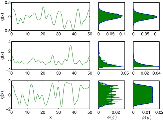
Fig. 1 Random thresholds. Realisations of the random threshold (left) for a Gaussian (top), shifted

ex-ponential (middle) and bump (bottom) distribution. The middle column shows the probability distribution of the threshold on the left. The right column depicts the probability distribution of the threshold obtained from 1000 realisations. Equation (9) was truncated after 50 (top), 32 (middle) and 64 (bottom) terms per sum, respectively. Parameter values areL=50,κ=3 andσ=0.2 (top),λ=1,μ= −1 (middle) and A=√2,B=2,α=0.5 (bottom)

towards the prescribed distributionφ (g), while keeping the chosen covariance func-tion exact in every iterafunc-tion step. In Fig.1we show the three types of distribution that we use to realise threshold values. These are (i) a Gaussian distribution, (ii) a highly skewed shifted exponential distribution, and (iii) a piecewise linear distribution with compact support. The precise mathematical form for each of these is given in Ap-pendixB.

3 Travelling Fronts

As mentioned in Sect.1much is now known about the effects of random forcing on neural field models. As regards travelling fronts the work of Bressloff and Webber [9] has shown that this can result in ‘fast’ perturbations of the front shape as well as a ‘slow’ horizontal displacement of the wave profile from its uniformly translat-ing position. A separation of time-scales method is thus ideally suited to analystranslat-ing this phenomenon, though we also note that more numerical techniques based upon stochastic freezing [33] could also be utilised. In this section we will explore the ef-fects of quenched or ‘frozen’ threshold noise on the properties of a travelling wave, and in particular its speed.

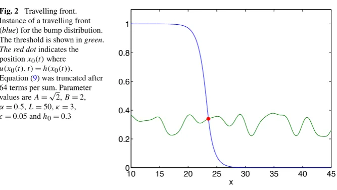
Fig. 2 Travelling front.

Instance of a travelling front (blue) for the bump distribution. The threshold is shown in green. The red dot indicates the positionx0(t )where

u(x0(t ), t )=h(x0(t )).

Equation (9) was truncated after 64 terms per sum. Parameter values areA=√2,B=2, α=0.5,L=50,κ=3, =0.05 andh0=0.3

state. In this case it is natural to define a pattern boundary as the interface between these two states. One way to distinguish between the high and the low activity state is by determining whetheruis above or below the firing threshold. When denoting the position of the moving interface byx0(t ), the above notion leads us to the defining equation

ux0(t ), t

=hx0(t )

. (12)

Here, we are assuming that there is only one point on the interface as illustrated in Fig.2, though in principle we could consider a set of points. For the choice (5) we see thatC(x)is differentiable at x=0, which means that the random threshold is differentiable in the mean square sense. The differentiation of (12) gives an exact expression for the velocity of the interfacecin the form

c≡dx0

dt = ut

hx−ux

x=x0(t )

, (13)

which modestly extends the original approach of Amari [21] with the inclusion of the term forhx. We can now describe the properties of a front solution solely in terms of the behaviour at the front edge that separates high activity from low, as described in [34,35]. To see this, let us consider a right moving front for whichu(x, t ) > h(x)for

x < x0(t )andu(x, t )≤h(x)forx≥x0(t ). Then we solve (3), dropping transients, to obtain

u(x, t )=

t

0

e−(t−s)ψ (x, s)ds, ψ (x, t )=

x0(t )

−∞ w(x−y)dy. (14)

Hence,

ux0(t ), t

=

t

0

dse−(t−s)

_∞

x0(t )−x0(s)

For simplicity we make the choicew(x)=exp(−|x|)/2 so that from (14) we find by differentiation with respect tox that for a right moving wave (for larget)

ux0(t ), t

= −ux|x=x0(t ). (16)

By noting that

ut|x=x0(t )= −h

x0(t )

+

x0(t )

−∞ w

x0(t )−y

dy= −hx0(t )

+1

2, (17)

and inserting (16) and (17) into (13), we find the wave speedc₊of a right moving wave

c₊= 1−2h(x0(t ))

2hx(x0(t ))+2h(x0(t ))

. (18)

When we repeat the above derivation for a left moving wave, the wave speedc₋is given by

c₋= 1−2h(x0(t ))

2hx(x0(t ))+2−2h(x0(t ))

, (19)

where we used

ux0(t ), t

=1+ux|x=x0(t ). (20) Note that in the case of a constant threshold with h(x)=h0 we obtain c₊ =

(1−2h0)/(2h0), forh0<1/2, andc₋=(1−2h0)/(2(1−h0)), for 1/2< h0<1, which recovers a previous result, as discussed in [16]. If the front is moving to the right we have an exact expression for the speed (see also [36]):

c(x)= 1−2h(x)

2h(x)+2hx(x)

. (21)

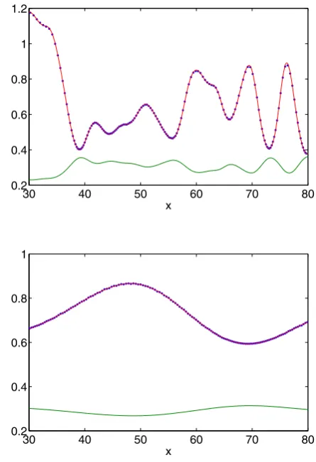
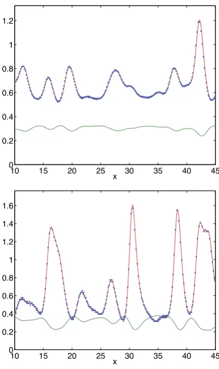
Examples of this relationship are shown in Figs.3 and4 where we plot bothc(x)

and the instantaneous front velocity extracted from a numerical simulation of (3). Figure3depicts results when the local probability distribution is a Gaussian for two different values of the correlation lengthκ, while Fig.4 illustrates travelling fronts for thresholds that are locally distributed as a skewed exponential and a bump. We see excellent agreement between the numerical values and the expression (21).

3.1 Perturbative Calculation of Wave Speed

We can also perturbatively calculate the effects of threshold disorder on the speed of a travelling front. Substituting (4) into (21) and taking 1 we find that

c(x)1−2h0

2h0 −

2h0

g(x)

h0 +

1−2h0

h0

g(x)

+ 2

2h2₀

g(x)2+2g(x)g(x)+g(x)2

h0 −

2g(x)g(x)−2g(x)2

Fig. 3 Instantaneous speed of a

travelling front for a Gaussian threshold distribution. Measured front speed for a Gaussian threshold distribution, extracted from a simulation of (3) (blue); theoretical value from (21) (red); and the threshold (4) (green), forκ=5 (top) and κ=30 (bottom). Equation (9) was truncated after 50 terms per sum. Other parameter values are σ2=1/κ,h0=0.3,=0.01,

L=100

where the prime denotes differentiation. We will now take the spatial and ensemble average of (22). It is convenient to introduce an angle bracket notation to denote spa-tial averaging according to· ≡₀L·dx/L. We find from (9) thatg =β0

√ λ0/L (since only the constant eigenfunctione(1)₀ (x)contributes to the integral and all other terms in (9) integrate to zero because of periodicity) andg =0 (because of period-icity). Hence, the spatial average ofctakes the compact form

c 1−2h0

2h0 −

g

2h2₀ + 2

2h3₀

g2+(1−2h0)

g2, (23)

where Lg2 = _m∞₌₀β_m2λm +

_∞

m=1γm2λm and Lg2 =

_∞

m=1βm2λmωm2 +

_∞

m=1γm2λmωm2. Now taking expectations over theβmandγmwe obtainE(g)=0,

LE(g2) =λ0+2∞_m=1λmandLE(g2) =2∞_m=1λmω2m. Hence, we may con-structc=E(c)as

c1−2h0

2h0 +

2 h3₀L

λ0 2 +

∞

m=1

λm+(1−2h0)

∞

m=1

λmω2m

Fig. 4 Instantaneous speed of a

travelling front for non-Gaussian threshold distributions. Measured front speed, extracted from a simulation of (3) (blue); theoretical value from (21) (red); and the threshold (4) (green) for a shifted exponential distribution (top) and a bump distribution (bottom) forκ=3, h0=0.3 andL=50.

Equation (9) was truncated after 32 (top) and 64 (bottom) terms per sum, respectively. Other parameter values areλ=1, μ= −1,= −0.03 (top) and A=√2,B=2,α=0.5, =0.05 (bottom)

This expression gives the lowest order correction term to the expression for speed (for a right moving wave) when the threshold is constant and takes the valueh0. The term in square brackets in (24) is positive, and thus spatial disorder will always increase the average speed. This term also increases as the correlation length decreases since theλm decay more slowly for smaller correlation lengths. Note, however, that the correction term remains uniformly small sinceλm∼κ for allmwhenκ 1.

distri-Fig. 5 Mean speed versusfor a Gaussian threshold

distribution.cas a function of forh0=0.3. Solid curve: (24);

circles: from averaging (21) over 1000 realisations per point. Equation (9) was truncated after 50 terms per sum. Other parameter values areκ=5, σ2=0.2,L=100

bution with the same variance. We again observe very good agreement between the small noise expansion (24) and averaging (21) for small values of. In addition, the curves for the Gaussian threshold and for the non-Gaussian thresholds obtained from averaging (21) almost agree, while the expansion (24) yields identical results for both kinds of threshold noise. The latter is a direct consequence of the bi-orthogonality of the Karhunen–Loève expansion. Equation (24) only depends on the eigenvalues of the covariance function and not on the properties of the local distributions.

4 Stationary Bumps

Neural fields of Amari type are known to support spatially localised stationary bump patterns when the anatomical connectivity function has a Mexican-hat shape. In a one dimensional spatial model, and in the absence of noise, it is known that pairs of bumps exist for some sufficiently low value of a constant threshold and that only the wider of the two is stable [21]. For random forcing it is possible to observe noise-induced drifting activity of bump attractors, which can be described by an effective diffusion coefficient (using a small noise expansion) [11] or by an anomalous sub-diffusive process in the presence of long-range spatio-temporal correlations [37]. However, it is also known that spatial disorder can act to pin states to certain network locations by breaking the (continuous) translation symmetry of the system, as described in [38] for neural field models with heterogeneous anatomical connectivity patterns. It is the latter phenomenon that we are interested in here, especially since for a disordered threshold that breaks translational symmetry, it is not a priori obvious how many bump solutions exist and what their stability properties are.

A one-bump solutionq(x)is characterised by a width, such that for two values

x1andx2with=x2−x1we haveq(x)≥h(x)forx1≤x≤x2. Using (3) a one-bump solution therefore satisfies

q(x)=

x2−x

x1−x

Fig. 6 Mean speed versusfor non-Gaussian threshold distributions.cas a function of forκ=0.5,h0=0.3,L=100

for the exponential distribution (top) and the bump distribution (bottom). In each panel results for the non-Gaussian distribution (dashed blue) are compared to those for a Gaussian distribution (solid green) with the same variance. Solid/dashed curves: (24); blue squares (non-Gaussian)/green circles (Gaussian): from averaging (21) over 1000 realisations per point.

Equation (9) was truncated after 250 terms per sum. Other parameter values areλ=1.66, μ= −0.6 (top) andA=√2, B=2,α=0.5 (bottom)

Note thath(x1)=q(x1)=h(x2)=q(x2)=U ()withU ()given by

U ()=

0

w|y|dy. (26)

We can determine the linear stability of bumps by studying the (linearised) evolution of a perturbationv(x)eλt _{around the stationary bumpq(x). We hence find from (3)}

(1+λ)v(x)=

Rw(x−y)δ

q(y)−h(y)v(y)dy (27)

=w(x−x1)

|Q(x1)|

v(x1)+

w(x−x2)

|Q(x2)|

v(x2), (28)

whereQ(x)=q(x)−h(x). Demanding that the perturbations atx1,2be non-trivial yields the spectral equation det(A−(1+λ)I2)=0, whereI2is the identity matrix inR2×2and

A=

_w(0)

|Q(x1)|

w()

|Q(x2)| w()

|Q(x1)| w(0)

|Q(x2)|

Fig. 7 Widths of stationary

bumps. The left hand side of (31) (solid) and the right hand side (dashed), withα=5, B=0.76,β=3,h0=0.05 and

=0

The eigenvalues are then given byλ=λ_±:

1+λ_±=1

2

TrA± (TrA)2_{−4 detA. (30)} Note further that forh(x)=0 we have|Q(x1)| = |Q(x2)| = |w(0)−w()|and thereforeλ₋=0 as expected from translation invariance.

4.1 Simple Heterogeneity

We first consider a simple form of heterogeneity to present the ideas, and then move to more general heterogeneity. Suppose w(x)=e−α(1−cosx)−Be−β(1−cosx) and

h(x)=h0+cosx, and the domain is [0,2π]. Then we have bumps which have their maximum at either 0 orπ. Suppose the maximum is at 0 and x1= −a for 0< a < π. Since we needh(x1)=h(x2)and the threshold is symmetric around 0, we immediately arrive atx2=a. To determineawe requireU ()=U (2a)=h(a) i.e.

2a 0

e−α(1−cosx)−Be−β(1−cosx)dx=h0+cosa. (31) Choosingα=5,B=0.76,β=3,h0=0.05 and=0 we have two bump widths, as shown in Fig.7(a=/2). We find that the larger root is stable and the other is unstable, and both have a zero eigenvalue as expected. Increasingfrom zero breaks the translational invariance of the system and we obtain 4 bumps for=0.01 as shown in Fig.8: the two that exist for the homogeneous case (=0), now centred aroundx =π, and similarly two centred around x =0. (We no longer restrict to

x1<0.)

4.2 General Heterogeneity

We keepw(x)=e−α(1−cosx)−Be−β(1−cosx)and now consider a generalh(x) with-out symmetries. The problem of the existence of a bump is this: givenh(x)and a value ofx1, find a value ofx2such thath(x2)=h(x1), andU ()=U (x2−x1)=

h(x1), whereU (x)is given by (26). This will not happen generically but only at iso-lated points in the(x1, x2)plane. Thus we need to solve the simultaneous equations

h(x2)=h(x1), (32)

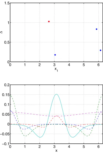
Fig. 8 Bump widths and

profiles for a spatially heterogeneous threshold. Top: solutions of (32)–(33), where =x2−x1, for

h(x)=0.05+0.01 cosx. Only the red solution is stable. Bottom: bump profiles for the solutions in the upper panel, and thresholdh(x)(dash-dotted). The solid bump is stable, all others (dashed) are unstable. Parameter values areα=5, B=0.76 andβ=3

and we only search for solutions which satisfy

0< x1<2π and x1< x2< x1+2π. (34) We now apply this general concept to the stochastic threshold (9). For each realisation and set of parameter values we use Newton’s method with 1000 randomly chosen ini-tial values which satisfy (34). Out of these 1000 initial values, the number of distinct solutions of (32)–(33) that satisfy (34) is recorded, and their stability is determined as described above. We then check these solutions to verify thatq(x) > h(x)only for

x1< x < x2. Any that do not satisfy this inequality are discarded.

Typical results for a Gaussian threshold are depicted in Fig.9 for κ =1 and

Fig. 9 Bump widths for a

Gaussian threshold distribution. Typical sets of solutions of (32)–(33) for a Gaussian threshold distribution with κ=1,σ=1 and=0.01. Only those with red dots are stable. Other parameter values are σ=1,α=5,B=0.76,β=3 andh0=0.05

Fig. 10 Bumps for a Gaussian

threshold distribution. Stable (solid) and unstable (dashed) solutions corresponding to the two points in Fig.9withx1

slightly less than 2. The threshold is shown dash-dotted. Parameter values areκ=1, =0.01,σ=1,α=5, B=0.76,β=3 andh0=0.05

In Fig.12we show the number of solutions of (32)–(33) as well as the number and fraction of stable solutions as a function of. While the number of solutions exhibits an increasing trend, the number of stable solutions decreases, leading to an overall decrease in the fraction of stable solutions. When lowering the correlation length five times (Fig.13), we observe a similar behaviour. Note, however, that the number of solutions has increased significantly. When we fixand varyκ the number of so-lutions decays quickly as shown in Fig.14. At the same time, the number of stable solutions remains almost constant, resulting in a strong increase of the fraction of stable solutions. Overall, we find that varying the amplitude of the threshold hetero-geneity by changingmore strongly affects solution numbers whenκ is small, and that the value ofκhas a significant effect on how many fixed points exist (and a lesser effect on the number of those which are stable).

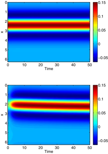
Fig. 11 Space-time plots of

bumps for a Gaussian threshold distribution. Simulations of (3) using as initial conditions the two different solutions shown in Fig.10. Top: stable; bottom: unstable. Parameter values are κ=1,=0.01,σ=1,α=5, B=0.76,β=3 andh0=0.05

When=0 bumps only exist below a critical value ofh0, and a branch of stable bumps coalesces with a branch of unstable bumps at this critical value whenh0 is varied. Figure16 shows results for a Gaussian threshold when we change h0 for

=0.002. We again observe two solution branches that only exist below a critical value ofh0. Each solution branch is smeared out compared to the homogeneous limit, indicating a probability distribution that has a finite and non-zero width.

Using the shifted exponential distribution for the threshold we obtain the results plotted in Fig. 17. We again observe two solution branches that emerge from the solutions in the homogeneous case asincreases, with the stable solutions confined to the upper branch. In contrast to the Gaussian case in Fig. 15the two solution branches do not grow symmetrically around the values of the homogeneous case. This is a manifestation of the highly skewed character of the exponential distribution compared to the symmetric Gaussian distribution. The probability distribution of the widths also exhibits much more structure compared to the Gaussian case.

Fig. 12 Bump solutions as a

function offor a Gaussian threshold distribution. Top: average number of total solutions (blue) and stable solutions (green) of (32)–(33) for a Gaussian threshold distribution. Bottom: fraction of solutions which are stable. Parameter values areα=5, B=0.76,β=3,h0=0.05,

κ=0.5 andσ2=4

different realisation ofh(x)and a different initial condition. We clearly see different “bands”, each identified with an integer number of bumps in a solution, and theL2

norm of these solutions increases as the number of bumps increases, in the same way as seen for systems with a smooth firing-rate function and homogeneous threshold [40–42], or with an oscillatory coupling function [39].

5 Conclusion

transfor-Fig. 13 Bump solutions as a

function offor a Gaussian threshold distribution. Top: average number of total solutions (blue) and stable solutions (green) of (32)–(33) for a Gaussian threshold distribution. Bottom: fraction of solutions which are stable. Parameter values areα=5, B=0.76,β=3,h0=0.05,

κ=0.1 andσ2=10

mationv(x, t )=u(x, t )−g(x). However, our approach permits the analysis of strong noise (see e.g. [20]) and hence will allow us to move beyond perturbative expansions.

Fig. 14 Bump solutions as a

function ofκfor a Gaussian threshold distribution Top: average number of total solutions (blue) and stable solutions (green) of (32)–(33) for a Gaussian threshold distribution. Bottom: fraction of solutions which are stable. Parameter values areα=5, B=0.76,β=3,h0=0.05,

=0.01 andσ2=1/κ

Competing Interests

The authors declare that they have no competing interests.

Authors’ Contributions

All authors contributed equally to the paper.

Acknowledgements SC was supported by the European Commission through the FP7 Marie Curie Initial Training Network 289146, NETT: Neural Engineering Transformative Technologies. We would like to thank Daniele Avitabile for useful feedback provided on a first draft of this manuscript.

Appendix A: Non-Gaussian Quenched Disorder

Fig. 15 Probability

distributions of bump widths for a Gaussian threshold

distribution. Top: log of the probability density ofvalues for a Gaussian threshold distribution. (White is high, black low.) Bottom: fraction of solutions which are stable. (Black=0, white=1.) Parameter values areα=5, B=0.76,β=3,h0=0.05,

κ=0.5 andσ2=4

findings for theαm to theβm andγm in (9) we note that this can be achieved by relabelling, i.e.

{α1, α2, α3, α4, . . .} = {β1, γ1, β2, γ2, . . .}. (35) In the following it is convenient to introduce the notationαm(k,l), which denotes the

mth expansion coefficient at thekth iteration for thelth realisation of the quenched disorder. To initialise the scheme, we generate M sets of uncorrelated αm(0,l), l= 1, . . . , M, drawn from the prescribed non-Gaussian distributionφ (g)shifted to mean zero and scaled to unit variance. A convenient way for doing this is to use inverse transform sampling based on the cumulative distribution functionFφofφ (g). Strictly speaking theαm(0,l)could be generated from any mean zero and unit variance distribu-tion, but starting with the prescribed distributionφ (g)might speed up convergence. For numerical purposes, the sum in (7) will only containN terms. One method to determineN is to impose the condition

max y

_∞

−∞

C(x, y)− N

m=1

λmem(x)em(y) dx

Fig. 16 Probability

distributions of bump widths for a Gaussian threshold

distribution. Top: probability density ofvalues for a Gaussian threshold distribution. (White is high, black low.) The deterministic solution is superimposed in blue. Bottom: fraction of solutions which are stable. (Black=0, white=1.) Parameter values areα=5, B=0.76,β=3,=0.002, κ=0.5 andσ2=4

i.e. that the maximalL1norm of the difference between the given covariance function and its approximation is smaller than someε >0. OnceNis fixed, each iteration step proceeds as follows:

1. GenerateMsamples of the quenched disorder

g(k,l)(x)=

N

m=1

λmαm(k,l)em(x), l=1, . . . , M, (37)

whereg(k,l)denotes thelth realisation of the quenched disorder at thekth itera-tion. Note that because theαm(k,l)are uncorrelated with unit variance, the numerical error in determining the covariance function only depends onN(to satisfy (8)) and onM(for high-fidelity averaging).

2. Numerically determine the cumulative distribution function

F_g(k)(y)= 1 M

M

l=1

Fig. 17 Probability

Fig. 18 Multibumps. Top:L2 norm of stable steady states of (3) for a Gaussian threshold distribution, with many different initial conditions, different realisations ofh(x), and various h0. Solutions indicated by blue

stars are shown in the bottom panel. Bottom: typical stable steady states solutions of (3) with 1, 2 and 3 bumps, for h0=0.03. TheirL2norms

increase as the number of bumps increases (blue dots in the top panel). These three solutions correspond to three different realisations ofh(x). Parameter values areα=15,B=0.76, β=9,=0.003,κ=0.5 and σ2=4

where Irepresents the indicator function, i.e. I(A)=1 if A is true, otherwise I(A)=0. The cumulative distribution functionFg(k)(y)generally does not agree with the prescribed functionFφ. The next two steps alleviate this problem. 3. Map the simulated valuesg(k,l)(x)to followFφ:

h(k,l)(x)=F_φ−1◦F_g(k)g(k,l)(x). (39) 4. Compute new valuesαm(k+1,l)as

α(k_m+1,l)=√1 λm

L

0

h(k,l)(x)−Eh(k,l)(x)em(x)dx. (40)

The mean ofα(km+1,l)is zero by construction, but the variance is unequal from one due to (39). Is therefore necessary to scale theαm(k+1,l)to have unit variance. 5. While theα(km+1,l)now give rise to the prescribed probability distributionφ (g),

they are correlated due to the mapping in (39). To decorrelate them, we use an iterative product-moment orthogonalisation technique.

that correlations between columns are minimised. This is equivalent to having minimal correlations between draws of theαm.

(b) Compute theN×N covariance matrixC(A)ofA.

(c) BecauseC(A)is positive definite, we can employ a Cholesky decomposition, i.e.C(A)=GTG. Therefore, the new matrixH=AG−1is uncorrelated. (d) Reorder the entries inAto follow the rankings inH.

Repeating the steps (a)–(d) will decrease the correlations of the α(km+1,l) as required.

Appendix B: Local Probability Distributions

We here provide details of the three zero-mean local probability distributions used in this study. We consider a Gaussian distribution

φ (x)=√ 1

2π σ2exp

− x2

2σ2

, −∞< x <∞, σ >0, (41)

a highly skewed shifted exponential distribution

φ (x)=exp−(λx+1), −1

λ≤x <∞, λ∈R, (42)

and a piecewise linear distribution with compact support

φ (x)=

⎧ ⎪ ⎨ ⎪ ⎩

α(L+x), −L≤x≤ −B, α(L−B), −B≤x≤B, α(L−x), B≤x≤L,

0< B < L, α >0. (43)

We refer to the last distribution as bump distribution. By demanding that it is nor-malised, we findα=1/(L2−B2). The variances of the exponential and bump dis-tribution are given, respectively, by

σ_SE2 = 1

λ2, σ

2 bu=

L2+B2

6 . (44)

References

1. Wilson HR, Cowan JD. Excitatory and inhibitory interactions in localized populations of model neu-rons. Biophys J. 1972;12:1–24.

2. Bressloff PC. Spatiotemporal dynamics of continuum neural fields. J Phys A. 2012;45:033001. 3. Coombes S, beim Graben P, Potthast R, Wright JJ, editors. Neural fields: theory and applications.

Berlin: Springer; 2014.

4. Webber MA, Bressloff PC. The effects of noise on binocular rivalry waves: a stochastic neural field model. J Stat Mech. 2013;3:P03001.

6. Hutt A, Longtin A, Schimansky-Geier L. Additive noise-induced Turing transitions in spatial systems with application to neural fields and the Swift–Hohenberg equation. Physica D. 2008;237:755–73. 7. Touboul J, Hermann G, Faugeras O. Noise-induced behaviors in neural mean field dynamics. SIAM

J Appl Dyn Syst. 2012;11:49–81.

8. Touboul J. Mean-field equations for stochastic firing-rate neural fields with delays: derivation and noise-induced transitions. Physica D. 2012;241:1223–44.

9. Bressloff PC, Webber MA. Front propagation in stochastic neural fields. SIAM J Appl Dyn Syst. 2012;11:708–40.

10. Bressloff PC. From invasion to extinction in heterogeneous neural fields. J Math Neurosci. 2012;2:6. 11. Kilpatrick ZP, Ermentrout B. Wandering bumps in stochastic neural fields. SIAM J Appl Dyn Syst.

2013;12:61–94.

12. Kilpatrick ZP, Faye G. Pulse bifurcations in stochastic neural field. SIAM J Appl Dyn Syst. 2014;13:830–60.

13. Kuehn C, Riedler MG. Large deviations for nonlocal stochastic neural fields. J Math Neurosci. 2014;4:1.

14. Poll DB, Kilpatrick ZP. Stochastic motion of bumps in planar neural fields. SIAM J Appl Math. 2015;75:1553–77.

15. Faugeras O, Inglis J. Stochastic neural field equations: a rigorous footing. J Math Biol. 2015;71:259– 300.

16. Bressloff PC. Waves in neural media: from single cells to neural fields. New York: Springer; 2014. 17. Inglis J, MacLaurin J. A general framework for stochastic traveling waves and patterns, with

applica-tion to neural field equaapplica-tions. SIAM J Appl Dyn Syst. 2016;15:195–234.

18. Krüger J, Stannat W. Front propagation in stochastic neural fields: a rigorous mathematical frame-work. SIAM J Appl Dyn Syst. 2014;13:1293–310.

19. Coombes S, Thul R, Laudanski J, Palmer AR, Sumner CJ. Neuronal spike-train responses in the presence of threshold noise. Front Life Sci. 2011;5:91–105.

20. Braun W, Matthews PC, Thul R. First-passage times in integrate-and-fire neurons with stochastic thresholds. Phys Rev E. 2015;91:052701.

21. Amari S. Dynamics of pattern formation in lateral-inhibition type neural fields. Biol Cybern. 1977;27:77–87.

22. Ermentrout GB, McLeod JB. Existence and uniqueness of travelling waves for a neural network. Proc R Soc Edinb. 1993;123A:461–78.

23. Coombes S. Waves, bumps and patterns in neural field theories. Biol Cybern. 2005;93:91–108. 24. Laing CR. Waves in spatially-disordered neural fields: a case study in uncertainty quantification.

In: Gomez D, Geris L, editors. Uncertainty in biology: a computational modeling approach. Berlin: Springer. 2014.

25. Shardlow T. Numerical simulation of stochastic PDEs for excitable media. J Comput Appl Math. 2005;175:429–46.

26. Le Maître OP, Knio OM. Spectral methods for uncertainty quantification: with applications to com-putational fluid dynamics. Dordrecht: Springer; 2010.

27. Papoulis A, Pillai SU. Probability, random variables and stochastic processes. 4th ed. Boston: McGraw-Hill; 2002.

28. Dietrich CR, Newsam GN. Fast and exact simulation of stationary Gaussian processes through circu-lant embedding of the covariance matrix. SIAM J Sci Comput. 1997;18:1088–107.

29. Shinozuka M, Deodatis G. Simulation of stochastic processes by spectral representation. Appl Mech Rev. 1991;44:191–204.

30. Phoon KK, Huang HW, Quek ST. Simulation of strongly non-Gaussian processes using Karhunen– Loeve expansion. Probab Eng Mech. 2005;20:188–98.

31. Yamazaki F, Shinozuka M. Digital generation of non-Gaussian stochastic fields. J Eng Mech. 1988;114:1183–97.

32. Li LB, Phoon KK, Quek ST. Comparison between Karhunen–Loeve expansion and translation-based simulation of non-Gaussian processes. Comput Struct. 2007;85:264–76.

33. Lord GJ, Thümmler V. Computing stochastic traveling waves. SIAM J Sci Comput. 2012;34:B24–43. 34. Coombes S, Schmidt H, Bojak I. Interface dynamics in planar neural field models. J Math Neurosci.

2012;2:9.

35. Bressloff PC, Coombes S. Neural ‘bubble’ dynamics revisited. Cogn Comput. 2013;5:281–94. 36. Coombes S, Laing CR, Schmidt H, Svanstedt N, Wyller JA. Waves in random neural media. Discrete

37. Qi Y, Breakspear M, Gong P. Subdiffusive dynamics of bump attractors: mechanisms and functional roles. Neural Comput. 2015;27:255–80.

38. Coombes S, Laing CR. Pulsating fronts in periodically modulated neural field models. Phys Rev E. 2011;83:011912.

39. Laing CR, Troy WC, Gutkin B, Ermentrout GB. Multiple bumps in a neuronal model of working memory. SIAM J Appl Math. 2002;63:62–97.

40. Coombes S, Lord GJ, Owen MR. Waves and bumps in neuronal networks with axo-dendritic synaptic interactions. Phys D, Nonlinear Phenom. 2003;178:219–41.

41. Rankin J, Avitabile D, Baladron J, Faye G, Lloyd DJ. Continuation of localized coherent structures in nonlocal neural field equations. SIAM J Sci Comput. 2014;36:B70–93.

42. Laing CR. PDE methods for two-dimensional neural fields. In: Coombes S, beim Graben P, Potthast R, Wright JJ, editors. Neural fields: theory and applications. Berlin: Springer; 2014.

43. Pinto DJ, Ermentrout GB. Spatially structured activity in synaptically coupled neuronal networks: I. Travelling fronts and pulses. SIAM J Appl Math. 2001;62:206–25.

44. González-Ramírez LR, Ahmed OJ, Cash SS, Wayne CE, Kramer MA. A biologically constrained, mathematical model of cortical wave propagation preceding seizure termination. PLoS Comput Biol. 2015;11:e1004065.

45. Huang X, Troy WC, Yang Q, Ma H, Laing CR, Schiff SJ, Wu J. Spiral waves in disinhibited mam-malian neocortex. J Neurosci. 2004;24:9897–902.