Four dimensional Fano toric complete intersections

rspa.royalsocietypublishing.org

Research

Cite this article:Coates T, Kasprzyk A, Prince T. 2015 Four-dimensional Fano toric complete

intersections.Proc. R. Soc. A471: 20140704.

http://dx.doi.org/10.1098/rspa.2014.0704

Received: 17 September 2014 Accepted: 23 December 2014

Subject Areas:

geometry

Keywords:

Fano manifolds, mirror symmetry, quantum differential equations, Picard–Fuchs equations

Author for correspondence:

T. Coates

e-mail:[email protected]

Electronic supplementary material is available at http://dx.doi.org/10.1098/rspa.2014.0704 or via http://rspa.royalsocietypublishing.org.

Four-dimensional Fano toric

complete intersections

T. Coates, A. Kasprzyk and T. Prince

Department of Mathematics, Imperial College London,

180 Queen’s Gate, London SW7 2AZ, UK

We find at least 527 new four-dimensional Fano manifolds, each of which is a complete intersection in a smooth toric Fano manifold.

1. Introduction

Fano manifolds are the basic building blocks of algebraic geometry, both in the sense of the Minimal Model Program [1–4] and as the ultimate source of most explicit examples and constructions. There are finitely many deformation families of Fano manifolds in each dimension [5]. There is precisely 1 one-dimensional Fano manifold: the line; there are 10 deformation families of two-dimensional Fano manifolds: the del Pezzo surfaces and there are 105 deformation families of three-dimensional Fano manifolds [6–13]. Very little is known about the classification of Fano manifolds in higher dimensions.

In this paper, we begin to explore the geography of Fano manifolds in dimension 4. Four-dimensional Fano manifolds of higher Fano index have been classified [6,14–22]—there are 35 in total—but the most interesting case, where the Fano variety has index 1, is wide open. We use computer algebra to find many four-dimensional Fano manifolds that arise as complete intersections in toric Fano manifolds in codimension at most 4. We find at least 738 examples, 717 of which have Fano index 1 and 527 of which are new.

Suppose that Y is a toric Fano manifold and that L1,. . .,Lc are nef line bundles on Ysuch that−KY−Λ is ample, where Λ=c1(L1)+ · · · +c1(Lc). Let X⊂Y be a smooth complete intersection defined by a regular section of⊕iLi. The Adjunction Formula gives that

−KX=(−KY−Λ)|X,

2015 The Authors. Published by the Royal Society under the terms of the Creative Commons Attribution Licensehttp://creativecommons.org/licenses/

by/4.0/, which permits unrestricted use, provided the original author and

2

rspa.r

oy

alsociet

ypublishing

.or

g

Proc

.R.

Soc

.A

47

1

:2

01

40

70

4

...

so X is Fano. We find all four-dimensional Fano manifolds X of this form such that the codimensioncis at most 4.

Our interest in this problem is motivated by a program to classify Fano manifolds in higher dimensions using mirror symmetry [23]. For each four-dimensional Fano manifoldXas above, therefore, we compute the essential ingredients for this program: the quantum period and regularized quantum differential equation associated to X, and a Laurent polynomialf that corresponds toXunder mirror symmetry; we also calculate basic geometric data aboutX, the ambient space Yand f. The results of our computations in machine-readable form, together with full details of our implementation and all source code used, can be found in the electronic supplementary material.

2. Finding four-dimensional Fano toric complete intersections

Our method is as follows. Toric Fano manifoldsYare classified up to dimension 8 by Batyrev et al.1[24–29]. For each toric Fano manifoldYof dimensiond=4+c, we:

(i) compute the nef cone ofY;

(ii) find allΛ∈H2(Y;Z) such thatΛis nef and−KY−Λis ample and

(iii) decomposeΛas the sum ofcnef line bundlesL1,. . .,Lcin all possible ways.

Each such decomposition determines a four-dimensional Fano manifoldX⊂Y, defined as the zero locus of a regular section of the vector bundle⊕iLi. To compute the nef cone in step (i), we consider dual exact sequences

0 // L // ZN ρ // _Zd // ₀

0 oo L oo D _(ZN₎ ρ _(Zd₎

o

o oo _0,

where the mapρ is defined by theNrays of a fanΣ forY. There are canonical identifications

L∼_=H2_(Y;Z)∼_{=Pic(Y), and the nef cone ofYis the intersection of cones} NC(Y)=

σ∈Σ

Di:i∈σ,

whereDiis the image underDof theith standard basis vector in (ZN)[30, proposition 15.1.3]. The classesΛin step (ii) are the lattice points in the polyhedronP=NC(Y)∩(−KY−NC(Y)) such that−KY−Λlies in the interior of NC(Y). Since NC(Y) is a strictly convex cone,Pis compact and the number of lattice points inPis finite. We implement step (iii) by first expressingΛas a sum of Hilbert basis elements in NC(Y) in all possible ways

Λ=b1+ · · · +br bian element of the Hilbert basis for NC(Y), (2.1)

where some of the bi may be repeated; this is a knapsack-style problem. We then, for each decomposition (2.1), partition thebiintocsubsetsS1,. . .,Scin all possible ways and define the line bundleLito be the sum of the classes inSi.

We found 117 173 distinct triples (X;Y;L1,. . .,Lc), with a total of 17 934 distinct ambient toric varieties Y. Note that the representation of a given Fano manifoldXas a toric complete intersection is far from unique: for example, ifXis a complete intersection inYgiven by a section

1_{Øbro’s method, which applies in all dimensions, starts with the observation that without loss of generality one cone in the}

3

rspa.r

oy

alsociet

ypublishing

.or

g

Proc

.R.

Soc

.A

47

1

:2

01

40

70

4

...

ofL1⊕ · · · ⊕Lcthen it is also a complete intersection inY×P1given by a section ofπ₁L1⊕ · · · ⊕

π

1Lc⊕π2OP1(1). Thus, we have found far fewer than 117 173 distinct four-dimensional Fano manifolds. We show below, by calculating quantum periods of the Fano manifoldsX, that we find at least 738 non-isomorphic Fano manifolds. Since the quantum period is a very strong invariant—indeed no examples of distinct Fano manifoldsX∼=Xwith the same quantum period GX=GXare known—we believe that we found precisely 738 non-isomorphic Fano manifolds. Eliminating the quantum periods found in [31], we see that at least 527 of our examples are new.

Remark 2.1. There exist Fano manifolds which do not occur as complete intersections in toric Fano manifolds. But in low dimensions, most Fano manifolds arise this way: 8 of the 10 del Pezzo surfaces, and at least 78 of the 105 smooth three-dimensional Fano manifolds, are complete intersections in toric Fano manifolds [32].

Remark 2.2. It may be the case that anyd-dimensional Fano manifold which occurs as a toric complete intersection in fact occurs as a toric complete intersection in codimensiond; we know of no counterexamples. But even if this holds in dimension 4, our search will probably not find all four-dimensional Fano manifolds which occur as toric complete intersections. This is because, if one of the line bundlesLiinvolved is nef but not ample, then the Kähler cone forXcan be strictly bigger than the Kähler cone forY. In other words, it is possible for−KXto be ample onXeven if −KY−Λis not ample onY. For an explicit example of this in dimension 3, see [32, §55].

3. Quantum periods and mirror Laurent polynomials

The quantum periodGXof a Fano manifoldXis a generating function

GX(t)=1+ ∞

d=1

cdtd t∈C, (3.1)

for certain genus-zero Gromov–Witten invariantscdofXwhich plays an important role in mirror symmetry. A precise definition can be found in [32, §B], but roughly speaking one can think ofcd as the ‘virtual number’ of rational curvesCinXthat pass through a given point, satisfy certain constraints on their complex structure, and satisfy−KX,C =d. The quantum period is discussed in detail in [23,32]; for us what will be important is that the regularized quantum period

ˆ

GX(t)=1+ ∞

d=1

d!cdtd t∈C,|t| ∞ (3.2)

satisfies a differential equation called theregularized quantum differential equationofX:

LXGˆX≡0 LX= m=N

m=0

pm(t)Dm, (3.3)

where thepmare polynomials andD=t(d/dt).

It has been proposed that Fano manifolds should correspond under mirror symmetry to Laurent polynomials which are extremal or of low ramification [23], in the sense discussed in §4. An n-dimensional Fano manifold X is said to be mirror-dual to a Laurent polynomial f∈C[x±₁1,. . .,x±n1] if the regularized quantum period ofXcoincides with the classical period off:

πf(t)= 1 (2πi)n

(S1₎n 1 1−tf

dx1

x1 · · · dxn

xn t∈C,|t| ∞.

4

rspa.r

oy

alsociet

ypublishing

.or

g

Proc

.R.

Soc

.A

47

1

:2

01

40

70

4

...

or asymplectomorphism of cluster type[33–35]:ϕf=g. We will write such a mutation asfϕ g. Mutations are known to preserve the classical period [33]: iffϕ gthenπf=πg.

Remark 3.1. In the paragraphs above we discuss the regularized quantum differential equation andthePicard–Fuchs differential equation. This involves choices of normalization. Our conventions are that the regularized quantum differential operator is the operatorLXas in (3.3) such that:

(i) the order,N, ofLXis minimal; (ii) the degree ofpN(t) is minimal;

(iii) the leading coefficient ofpNis positive; and

(iv) the coefficients of the polynomialsp0,. . .,pNare integers with greatest common divisor equal to 1.

The Picard–Fuchs differential operator is the differential operatorLf such that:

Lfπf≡0 Lf= m=N

m=0

Pm(t)Dm,

where thePmare polynomials andD=t(d/dt), and that the analogues of conditions (i)–(iv) above hold.

We determined the quantum period GX, for each of the triples (X;Y;L1,. . .,Lc) from §2, as follows. For each such triple we found, using the Mirror Theorem for toric complete intersections [36] and a generalization of a technique due to V. Przyjalkowski, a Laurent polynomialfthat is mirror-dual toX. This process is described in detail in §5. We then computed, for each triple, the first 20 terms of the power series expansion of GXˆ =πf using the Taylor expansion

πf(t)= ∞

d=0

αdtd,

whereαd is the coefficient of the unit monomial infd. We divided the 117 173 triples into 738 ‘buckets’, according to the value of the first 20 terms of the power series expansion ofGˆX=πf, and then proved that any two Fano manifoldsX,Xin the same bucket have the same quantum period by exhibiting a chain of mutations fϕ0 f1ϕ1 · · ·

ϕn−1

fnϕn gthat connects the Laurent polynomialsfandgmirror-dual toXandX.

For each quantum period GX, we computed the quantum differential operator LX directly from the mirror Laurent polynomialfchosen above, using Lairez’s generalized Griffiths–Dwork algorithm [37]. The output from Lairez’s algorithm is a differential operatorL=N_m=0Pm(t)Dm withP0,. . .,PN∈Q[t] such that, with very high probability,Lπf≡0. Such an operatorLgives a recurrence relation for the Taylor coefficientsα0,α1,α2. . .ofπf; using this recurrence relation and the first 20 Taylor coefficients computed above, we solved for the first 2000 Taylor coefficientsαk. We then consider an operator

¯ L=

¯ N

m=0

¯ Pm(t)Dm,

5

rspa.r

oy

alsociet

ypublishing

.or

g

Proc

.R.

Soc

.A

47

1

:2

01

40

70

4

...

is not proven—partly because Lairez’s algorithm relies on a randomized interpolation scheme that is not guaranteed to produce an operator annihilatingπf, and partly because ifLf were to involve polynomialsPmof extremely large degree, 2000 terms of the Taylor expansion ofπfwill not be enough to detectLf. The operatorsL¯ that we found satisfy a number of delicate conditions that act as consistency checks: for example they are of Fuchsian type (which is true forLf, asLf arises geometrically from a variation of Hodge structure). Thus, we are confident thatL¯=Lf in every case.2 SinceGXˆ =πf andLX=Lf by construction, this determines, with high confidence, the quantum periodGXand the regularized quantum differential operatorLX.

Remark 3.2. The use of Laurent polynomials and Lairez’s algorithm is essential here. There is a closed formula [32, corollary D.5] for the quantum period of the Fano manifolds that we consider, and one could in principle use this together with the linear algebra calculation described above to compute (a good candidate for) the regularized quantum differential operatorLX. In practice, however, for many of the examples that we treat here, it is impossible to determine enough Taylor coefficients from the formula: the computations involved are well beyond the reach of current hardware, both in terms of memory consumption and runtime. By contrast, our approach using mirror symmetry and Lairez’s algorithm will run easily on a desktop PC.

Remark 3.3. The regularized quantum differential equation for X coincides with the (unregularized) quantum differential equation for an anticanonical Calabi–Yau manifoldZ⊂X. The study of the regularized quantum period from this point of view was pioneered by Batyrev et al.[39,40] and an extensive study of fourth-order Calabi–Yau differential operators was made in [41]. We found 26 quantum differential operators with N=4; these coincide with or are equivalent to the fourth-order Calabi–Yau differential operators with AESZ IDs 1, 3, 4, 5, 6, 15, 16, 17, 18, 19, 20, 21, 22, 23, 34, 369, 370 and 424 in the Calabi–Yau Operators Database [42], together with one new fourth-order Calabi–Yau differential operator (which corresponds to our period sequence with ID 469).

4. Ramification data

Consider now one of our regularized quantum differential operators

LX= m=N

m=0

pm(t)Dm

as in (3.3), and its local systemV→P1\Sof solutions. HereS⊂P1is the set of singular points of the regularized quantum differential equation.

Definition 4.1 ([23]). LetS⊂P1_{be a finite set andV→P}1_{\Sa local system. Fix a basepoint}

x∈P1_{\S. Fors∈S, choose a small loop that winds once anticlockwise aroundsand connect it to}

xvia a path, thereby making a loopγsaboutsbased atx. LetTs:Vx→Vxdenote the monodromy ofValongγs. TheramificationofVis

rf(V) := s∈S

dim

Vx/VxTs

.

The ramification rf(V) is independent of the choices of basepoint xand of small loopsγs. A non-trivial, irreducible local systemV→P1\Shas rf(V)≥2rk(V): see [23, §2].

Definition 4.2. LetV→P1_{\S be a local system as above. Theramification defectofVis the} quantity rf(V)−2rk(V). A local system of ramification defect zero is calledextremal.

Definition 4.3. Theramification(respectively,ramification defect) of a differential operatorLXis the ramification (respectively, ramification defect) of the local system of solutionsLXf≡0.

6

rspa.r

oy

alsociet

ypublishing

.or

g

Proc

.R.

Soc

.A

47

1

:2

01

40

70

4

...

Table 1.Ramification defects for 575 of the 738 regularized quantum differential operators.

. . . .

ramification defect 0 1 2 3

. . . .

number of occurrences 92 290 167 26

. . . .

To compute the ramification of LX, we proceed as in [31]. One can compute Jordan normal forms of the local log-monodromies{logTs:s∈S}using linear algebra over a splitting fieldkfor pN(t). (Every singular point ofLXis defined overk.) This is classical, going back to Birkhoff [43], as corrected by Gantmacher [44, vol. 2, §10] and Turrittin [45]; a very convenient presentation can be found in the book of Kedlaya [46, §7.3]. In practice, we use the symbolic implementation ofQprovided by the computational algebra system Magma [47,48]. We computed ramification data for 575 of the 738 regularized quantum differential operators, finding ramification defects as shown in table 1; this lends some support to the conjecture, due to Golyshev [23], that a Laurent polynomial f which is mirror-dual to a Fano manifold should have a Picard–Fuchs operatorLf that is extremal or of low ramification. For the remaining 163 regularized quantum differential operators, the symbolpN(t) contains a factor of extremely high degree. This makes the computation of ramification data prohibitively expensive.

5. The Przyjalkowski method

We now explain, given complete intersection data (X;Y;L1,. . .,Lc) as in §2, how to find a Laurent polynomialfthat is mirror-dual toX. This is a slight generalization of a technique that we learned from V. Przyjalkowski3 [50,51], and which is based on the mirror theorems for toric complete intersections due to Givental [36] and Horiet al.[52]. Recall the exact sequence

0 oo L oo D _(ZN₎ oo ρ _(Zd₎ oo ₀

from §2 and the elementsDi∈L, 1≤i≤N, defined by the standard basis elements of (ZN). Recall further thatL∼=Pic(Y), so that each line bundleLm defines a class inL. Suppose that there exists a choice of disjoint subsetsE,S1,. . .,Scof{1, 2,. . .,N}such that:

— {Dj:j∈E}is a basis forL;

— eachLmis a non-negative linear combination of{Dj:j∈E}; and — _k∈SmDk=Lmfor eachm∈ {1, 2,. . .,c};

and choose distinguished elementssm∈Sm, 1≤m≤c. SetS◦_m=Sm\ {sm}. Writing the mapDin terms of the standard basis for (ZN)and the basis{Dj:j∈E}forLdefines an (N−d)×Nmatrix (mji) of integers. Let (x1,. . .,xN) denote the standard coordinates on (C×)N, letr=N−d, and defineq1,. . .,qrandF1,. . .,Fcby

qj= N

i=1

xm_iji Fm= k∈Sm

xk.

Givental [36] and Horiet al.[52] have shown that

GX=

Γe

tW

_N

i=1(dxi/xi)

_c

m=1 dFm∧

_r

j=1(dqj/qj)

, (5.1)

7

rspa.r

oy

alsociet

ypublishing

.or

g

Proc

.R.

Soc

.A

47

1

:2

01

40

70

4

...

whereW=x1+ · · · +xNandΓ is a certain cycle in the submanifold of (C×)Ndefined by

q1= · · · =qr=1 F1= · · · =Fc=1.

Introducing new variablesyifori∈ c_m=1S◦_m, setting

xi=

⎧ ⎪ ⎪ ⎪ ⎨ ⎪ ⎪ ⎪ ⎩

1 1+_k∈S◦

myk

ifi=sm

yi 1+_k∈S◦

myk

ifi∈S◦_m.

and using the relationsq1= · · · =qr=1 to eliminate the variablesxj,j∈E, allows us to writeW−c as a Laurent polynomialfin the variables

{yi:i∈ c_m=1S◦m} and {xi:i∈Eandi∈ cm=1S◦m}.

The mirror theorem (5.1) then implies thatGXˆ =πf, or in other words thatfis mirror-dual toX. The Laurent polynomial f produced by Przyjalkowski’s method depends on our choices of E,S1,. . .,Sc, ands1,. . .,sc, but up to mutation this is not the case:

Theorem 5.1 ([53]). Let Y be a toric Fano manifold and let L1,. . .,Lcbe nef line bundles on Y such that−KY−Λis ample,whereΛ=c1(L1)+ · · · +c1(Lc). Let X⊂Y be a smooth complete intersection

defined by a regular section of⊕iLi. Let f and g be Laurent polynomial mirrors to X obtained by applying Przyjalkowski’s method to(X;Y;L1,. . .,Lc) as above,but with possibly different choices for the subsets

E,S1,. . .,Scand the elements s1,. . .,sc. Then there exists a mutationϕsuch that f

ϕ

g.

Example 5.2. LetYbe the projectivization of the vector bundleO⊕2_⊕O(1)⊕2_overP2_{. Choose} a basis for the two-dimensional latticeLsuch that the matrix (mji) of the mapDis

1 1 1 0 0 1 1

0 0 0 1 1 1 1

.

Consider the line bundleL1→Ydefined by the element (2, 1)∈L, and the Fano hypersurface

X⊂Ydefined by a regular section ofL1. Applying Przyjalkowski’s method to the triple (X;Y;L1) withE= {3, 4},S1= {1, 2, 5}ands1=1 yields the Laurent polynomial

f=(1+y2+y5)2 y2x6x7 +

1+y2+y5

y5x6x7 +x6+x7

mirror-dual toX. Applying the method withE= {3, 4},S1= {1, 6}ands1=1 yields

g=x2+(1+y6) 2

x2y6x7 + 1+y6

x5y6x7 +x5+x7.

We have thatfϕ gwhere the mutationϕ: (C×)4_→(C×₎4_{is given by} (x2,x5,y6,x7)→

x2

x5y6, 1

y6,x7,x2+x5

=(y2,y5,x6,x7).

8

rspa.r

oy

alsociet

ypublishing

.or

g

Proc

.R.

Soc

.A

47

1

:2

01

40

70

4

6. Examples

(a) The cubic fourfold

Let X be the cubic fourfold. This arises in our classification from the complete intersection data (X;Y;L) withY=P5andL=O_P5(3). The Przyjalkowski method yields [54, §2.1] a Laurent polynomial

f=(1+x+y)

3

xyzw +z+w

mirror-dual toX, and elementary calculation gives

πf(t)= ∞

d=0

(3d)!(3d)! (d!)6 t

3d_.

ThusGXˆ =πf, and the corresponding regularized quantum differential operator is

LX=D4−729t3(D+1)2(D+2)2.

The local log-monodromies for the local system of solutionsLXg≡0 are

⎛ ⎜ ⎜ ⎜ ⎝

0 1 0 0

0 0 1 0

0 0 0 1

0 0 0 0

⎞ ⎟ ⎟ ⎟

⎠ att=0

⎛ ⎜ ⎜ ⎜ ⎝

0 0 0 0

0 0 0 0

0 0 0 1

0 0 0 0

⎞ ⎟ ⎟ ⎟

⎠ att=19

⎛ ⎜ ⎜ ⎜ ⎝

0 0 0 0

0 0 0 0

0 0 0 1

0 0 0 0

⎞ ⎟ ⎟ ⎟

⎠ at the roots of 81t2+9t+1=0

⎛ ⎜ ⎜ ⎜ ⎝

0 1 0 0

0 0 0 0

0 0 0 1

0 0 0 0

⎞ ⎟ ⎟ ⎟

⎠ att= ∞

and the operatorLXis extremal.

(b) A (3,3) complete intersection in

P

6

LetXbe a complete intersection inY=P6of type (3, 3). This arises in our classification from the complete intersection data (X;Y;L1,L2) withL1=L2=OP6(3). The Przyjalkowski method yields a Laurent polynomial

f=(1+x+y)

3_(1+z+w)3

xyzw −36

mirror-dual toX, and [32, corollary D.5] gives

ˆ

GX=πf(t)= ∞ k=0 ∞ l=0

(3l)!(3l)!(k+l)! k!(l!)7 (−36)

9

rspa.r

oy

alsociet

ypublishing

.or

g

Proc

.R.

Soc

.A

47

1

:2

01

40

70

4

...

0 100 200 300 400 500 600 700 800

0 5 10 15

degree

frequenc

y

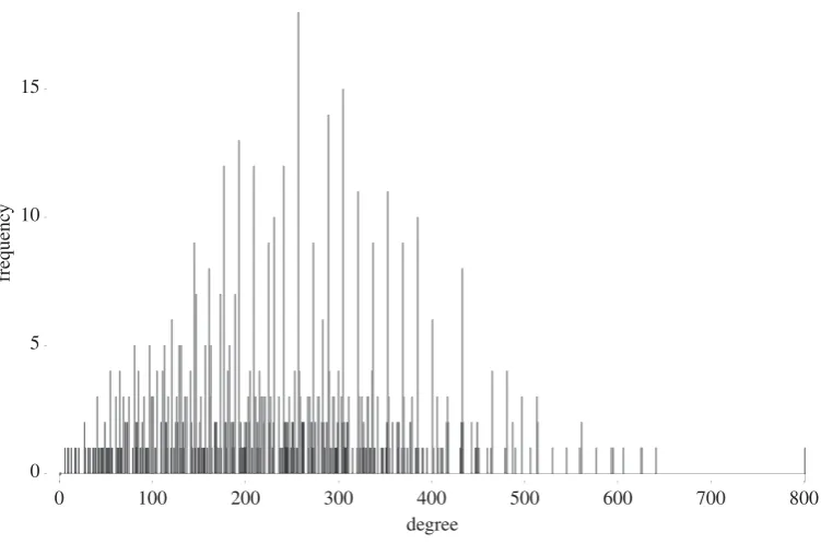
Figure 1.The distribution of degrees (frequency plot).

The corresponding regularized quantum differential operatorLXis

(36t+1)4(693t−1)D4

+ 18t(36t+1)3(13 860t+61)D3

+ 9t(36t+1)2(3 492 720t2+57 672t+77)D2

+ 144t(36t+1)(11 226 600t3+377 622t2+2754t+1)D + 15 552t2(1 796 256t3+98 496t2+1605t+7).

The local log-monodromies for the local system of solutionsLXg≡0 are

⎛ ⎜ ⎜ ⎜ ⎝

0 1 0 0

0 0 1 0

0 0 0 1

0 0 0 0

⎞ ⎟ ⎟ ⎟

⎠ att=0

⎛ ⎜ ⎜ ⎜ ⎝

0 0 0 0

0 0 0 0

0 0 0 1

0 0 0 0

⎞ ⎟ ⎟ ⎟

⎠ att=6931

⎛ ⎜ ⎜ ⎜ ⎝

2

3 1 0 0

0 2₃ 0 0

0 0 1₃ 1

0 0 0 1₃

⎞ ⎟ ⎟ ⎟

⎠ att= −361

10

rspa.r

oy

alsociet

ypublishing

.or

g

Proc

.R.

Soc

.A

47

1

:2

01

40

70

4

...

0 100 200 300 400 500 600 700 800

0 100 200 300 400 500 600 700

degree

cumulati

v

e frequenc

y

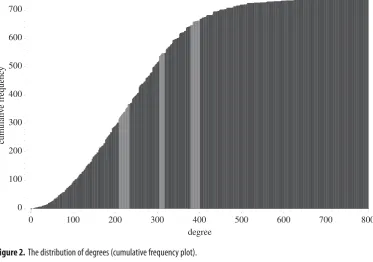
Figure 2.The distribution of degrees (cumulative frequency plot).

200 400 600 800

4 6 8 10 12

degree N

Figure 3.The distribution of degrees withN.

7. Results and analysis

We close by indicating how basic numerical invariants—degree and size of cohomology—vary across the 738 families of Fano manifolds that we have found. The degree (−KX)4varies from 5 to 800, as shown in figures1and2.

We do not have direct access to the size of the cohomology algebra of our Fano manifoldsX, as many of the line bundles occurring in the complete intersection data (X;Y;L1,. . .,Lc) are not ample and so the Lefschetz theorem need not apply. But the orderNof the regularized quantum differential operator is a good proxy for the size of the cohomology.Nis the rank of a certain local system—an irreducible piece of the Fourier–Laplace transform of the restriction of the Dubrovin connection (in the Frobenius manifold given by the quantum cohomology ofX) to the line inH•(X) spanned by−KX—and in the case where this local system is irreducible, which is typical,Nwill coincide with the dimension ofH•(X). For our examples,Nlies in the set{4, 6, 8, 10, 12}.Figure 3 shows howNvaries with the degree (−KX)4, with darker grays indicating a larger number of examples with thatNand degree.

The isolated example on the right offigure 3, withN=6 and degree 800, is the blow up of

11

rspa.r

oy

alsociet

ypublishing

.or

g

Proc

.R.

Soc

.A

47

1

:2

01

40

70

4

...

200 400 600 800

4

6 8

10

12

degree

N

Figure 4.The distribution of degrees withN, with toric Fano manifolds highlighted.

200 400 600 800

–100 0 100 200 300 400 500 600 700 800

degree

E

ul

er n

u

mber

Figure 5.The distribution of degrees with Euler number.

12

rspa.r

oy

alsociet

ypublishing

.or

g

Proc

.R.

Soc

.A

47

1

:2

01

40

70

4

...

complete intersection of type (3, 3) inP6, withχ=369. The three examples with the most negative Euler number areP1×V₄3whereV3₄is a quartic hypersurface inP4, withχ= −112;P1×V₆3where V3₆is a complete intersection of type (2, 3) inP5, withχ= −72; andP1×V₈3whereV3₈is a complete intersection of type (2, 2, 2) inP6, withχ= −48.

Ethics statement. This research did not involve human or animal subjects.

Data accessibility. The Electronic Supplementary Material contains the results of our computations, in machine readable form, together with full source code written in Magma [47]. See the files calledREADME.txtfor details. The source code and data, but not the text of this paper, are released under a Creative Commons CC0 license (Creative Commons CC0 license,https://creativecommons.org/publicdomain/zero/1.0/andhttps:// creativecommons.org/publicdomain/zero/1.0/legalcode.): see the files calledCOPYING.txtfor details. If you make use of the source code or data in an academic or commercial context, you should acknowledge this by including a reference or citation to this paper.

Acknowledgements. The computations underlying this work were performed using the Imperial College High Performance Computing Service and the compute cluster at the Department of Mathematics, Imperial College London. We thank Simon Burbidge, Matt Harvey and Andy Thomas for valuable technical assistance. We thank John Cannon and the Computational Algebra Group at the University of Sydney for providing licenses for the computer algebra system Magma. We thank Alessio Corti for a number of very useful conversations, Pierre Lairez for explaining his generalized Griffiths–Dwork algorithm and sharing his code with us, and Duco van Straten for his analysis of the regularized quantum differential operators withN=4.

Author contributions. T.C., T.P. and A.K. performed the research and wrote the paper.

Funding statement. This research was supported by a Royal Society University Research Fellowship; the Leverhulme Trust; ERC Starting Investigator Grant number 240123; EPSRC grant EP/I008128/1; an EPSRC Small Equipment grant; and an EPSRC Prize Studentship.

Competing interests. We have no competing interests.

References

1. Reid M. 2002 Update on 3-folds. InProc. Int. Congress of Mathematicians, Beijing, 2002, vol. II, pp. 513–524. Beijing, China: Higher Ed. Press.

2. Corti A (ed.) 2007Flips for 3-folds and 4-folds. Oxford Lecture Series in Mathematics and its Applications, vol. 35. Oxford, UK: Oxford University Press.

3. Birkar C, Cascini P, Hacon CD, McKernan J. 2010 Existence of minimal models for varieties of log general type.J. Am. Math. Soc.23, 405–468. (doi:10.1090/S0894-0347-09-00649-3)

4. Hacon CD, McKernan J. 2010 Existence of minimal models for varieties of log general type. II. J. Am. Math. Soc.23, 469–490. (doi:10.1090/S0894-0347-09-00651-1)

5. Kollár J, Miyaoka Y, Mori S. 1992 Rational connectedness and boundedness of Fano manifolds. J. Differ. Geom.36, 765–779.

6. Iskovskih VA. 1977 Fano threefolds. I.Izv. Akad. Nauk SSSR Ser. Mat.41, 516–562, 717. 7. Iskovskih VA. 1978 Fano threefolds. II.Izv. Akad. Nauk SSSR Ser. Mat.42, 506–549.

8. Iskovskih VA. 1979 Anticanonical models of three-dimensional algebraic varieties. Current problems in mathematics, vol. 12, pp. 59–157. (Russian) Moscow, Russia: VINITI; 239 (loose errata).

9. Mori S, Mukai S. 1981/82 Classification of Fano 3-folds withB2≥2.Manuscr. Math.36, 147– 162. (doi:10.1007/BF01170131)

10. Mori S, Mukai S. 1983 On Fano 3-folds withB2≥2. InAlgebraic varieties and analytic varieties (Tokyo, 1981),Adv. Stud. Pure Math., vol. 1, pp. 101–129. Amsterdam, The Netherlands: North-Holland.

11. Mori S, Mukai S. 1986 Classification of Fano 3-folds withB2≥2. I. InAlgebraic and topological

theories(Kinosaki, 1984), pp. 496–545. Tokyo, Japan: Kinokuniya.

12. Mori S, Mukai S. 2003 Erratum: ‘Classification of Fano 3-folds withB2≥2’ (Manuscr. Math.36 (1981/82), no. 2, 147–162).Manuscr. Math.110, 407. (doi:10.1007/s00229-002-0336-2)

13. Mori S, Mukai S. 2004Extremal rays and Fano 3-folds, pp. 37–50. The Fano Conf., University Torino, Turin.

14. Shokurov VV. 1985 A nonvanishing theorem.Izv. Akad. Nauk SSSR Ser. Mat.49, 635–651. 15. Kobayashi S, Ochiai T. 1973 Characterizations of complex projective spaces and

hyperquadrics.J. Math. Kyoto Univ.13, 31–47.

13

rspa.r

oy

alsociet

ypublishing

.or

g

Proc

.R.

Soc

.A

47

1

:2

01

40

70

4

...

17. Serpico ME. 1980 Fano varieties of dimensionsn≥4 and of indexr≥n−1.Rend. Sem. Mat. Univ. Padova62, 295–308.

18. Fujita T. 1980 On the structure of polarized manifolds with total deficiency one. I.J. Math. Soc. Japan32, 709–725. (doi:10.2969/jmsj/03240709)

19. Fujita T. 1981 On the structure of polarized manifolds with total deficiency one. II.J. Math. Soc. Japan33, 415–434. (doi:10.2969/jmsj/03330415)

20. Fujita T. 1984 On the structure of polarized manifolds with total deficiency one. III.J. Math. Soc. Japan36, 75–89. (doi:10.2969/jmsj/03610075)

21. Fujita T. 1990Classification theories of polarized varieties. London Mathematical Society Lecture Note Series, vol. 155. Cambridge, UK: Cambridge University Press.

22. Iskovskikh VA, Prokhorov YuG. 1999 Fano varieties. Algebraic geometry, V, Encyclopaedia Math. Sci., vol. 47, pp. 1–247. Berlin, Germany: Springer.

23. Coates T, Corti A, Galkin S, Golyshev V, Kasprzyk AM. 2014 Mirror symmetry and Fano manifolds. InEuropean Congress of Mathematics Kraków, 2–7 July 2012, pp. 285–300.

24. Batyrev VV. 1981 Toric Fano threefolds.Izv. Akad. Nauk SSSR Ser. Mat.45, 704–717, 927. 25. Watanabe K, Watanabe M. 1982 The classification of Fano 3-folds with torus embeddings.

Tokyo J. Math.5, 37–48. (doi:10.3836/tjm/1270215033)

26. Batyrev VV. 1999 On the classification of toric Fano 4-folds.J. Math. Sci.(New York)94, 1021– 1050. Algebraic geometry, 9. (doi:10.1007/BF02367245)

27. Sato H. 2000 Toward the classification of higher-dimensional toric Fano varieties. Tohoku Math. J.52, 383–413. (doi:10.2748/tmj/1178207820)

28. Kreuzer M, Nill B. 2009 Classification of toric Fano 5-folds. Adv. Geom. 9, 85–97. (doi:10.1515/ADVGEOM.2009.005)

29. Øbro M. 2007 An algorithm for the classification of smooth Fano polytopes. (http://arxiv.org/ abs/0704.0049)

30. Cox DA, Little JB, Schenck HK. 2011Toric varieties. Graduate Studies in Mathematics, vol. 124. Providence, RI: American Mathematical Society.

31. Coates T, Galkin S, Kasprzyk AM, Strangeway A. 2014 Quantum periods for certain four-dimensional Fano manifolds. (http://arxiv.org/abs/1406.4891)

32. Coates T, Corti A, Galkin S, Kasprzyk AM. 2013 Quantum periods for 3-dimensional Fano manifolds. (http://arxiv.org/abs/1303.3288)

33. Akhtar M, Coates T, Galkin S, Kasprzyk AM. 2012 Minkowski polynomials and mutations. SIGMA Symmetry Integrability Geom. Methods Appl. 8, Paper 094, 17. (doi:10.3842/SIGMA. 2012.094)

34. Galkin S, Usnich A. 2010 Mutations of potentials. Preprint IPMU 10-0100.

35. Katzarkov L, Przyjalkowski V. 2012 Landau-Ginzburg models—old and new. InProc. Gökova Geometry-Topology Conf. 2011, pp. 97–124. Somerville, MA: Int. Press.

36. Givental A. 1998 A mirror theorem for toric complete intersections. InTopological field theory, primitive forms and related topics(Kyoto, 1996), Progr. Math., vol. 160, pp. 141–175. Boston, MA: Birkhäuser Boston.

37. Lairez P. 2014 Computing periods of rational integrals. (http://arxiv.org/abs/1404.5069) Source code available fromhttps://github.com/lairez/periods.

38. van Hoeij M. 1997 Factorization of differential operators with rational functions coefficients. J. Symb. Comput.24, 537–561. (doi:10.1006/jsco.1997.0151)

39. Batyrev VV, Ciocan-Fontanine I, Kim B, van Straten D. 1998 Conifold transitions and mirror symmetry for Calabi-Yau complete intersections in Grassmannians.Nuclear Phys. B514, 640– 666. (doi:10.1016/S0550-3213(98)00020-0)

40. Batyrev VV, Ciocan-Fontanine I, Kim B, van Straten D. 2000 Mirror symmetry and toric degenerations of partial flag manifolds.Acta Math.184, 1–39. (doi:10.1007/BF02392780) 41. Almkvist G, van Enckevort C, van Straten D, Zudilin W. 2005 Tables of Calabi–Yau equations.

(arXiv:math/0507430[math.AG])

42. van Straten D. Calabi-Yau Operators Database, online, access via http://www.mathematik. uni-mainz.de/CYequations/db/.

43. Birkhoff GD. 1913 Equivalent singular points of ordinary linear differential equations.Math. Ann.74, 134–139. (doi:10.1007/BF01455347)

44. Gantmacher FR. 1959The theory of matrices, vols. 1, 2 (translated by KA Hirsch). New York, NY: Chelsea Publishing Co.

14

rspa.r

oy

alsociet

ypublishing

.or

g

Proc

.R.

Soc

.A

47

1

:2

01

40

70

4

...

46. Kedlaya KS. 2010p-adic differential equations. Cambridge Studies in Advanced Mathematics, vol. 125. Cambridge, UK: Cambridge University Press.

47. Bosma W, Cannon J, Playoust C. 1997 The Magma algebra system. I. The user language. J. Symb. Comput.24, 235–265. Computational algebra and number theory (London, 1993). (doi:10.1006/jsco.1996.0125)

48. Steel AK. 2010 Computing with algebraically closed fields. J. Symb. Comput. 45, 342–372. (doi:10.1016/j.jsc.2009.09.005)

49. Katzarkov L. 2009 Homological mirror symmetry and algebraic cycles. InHomological mirror symmetry. Lecture Notes in Phys., vol. 757, pp. 125–152. Berlin, Germany: Springer.

50. Przyjalkowski V. 2011 Hori-Vafa mirror models for complete intersections in weighted projective spaces and weak Landau-Ginzburg models. Cent. Eur. J. Math. 9, 972–977. (doi:10.2478/s11533-011-0070-7)

51. Przhiyalkovski˘ı VV. 2013 Weak Landau-Ginzburg models of smooth Fano threefolds.Izv. Ross. Akad. Nauk Ser. Mat.77, 135–160.

52. Hori K, Katz S, Klemm A, Pandharipande R, Thomas R, Vafa C, Vakil R, Zaslow E. 2003Mirror symmetry. Clay Mathematics Monographs, vol. 1. Providence, RI: American Mathematical Society; Clay Mathematics Institute, Cambridge, MA. With a preface by Vafa.

53. Prince T. (In preparation) PhD thesis, Imperial College, London, UK.