Coordinate based random effect size meta analysis of neuroimaging studies

Coordinate Based Random Effect Size meta-analysis of neuroimaging studies

Tench CR1*

[email protected]

Radu Tanasescu1,2

[email protected]

Constantinescu CS 1

[email protected] Auer DP3

[email protected]

Cottam WJ3

[email protected]

1_{Division of Clinical Neurosciences, Clinical Neurology, University of Nottingham, Queen's Medical}

Centre, Nottingham, UK

2_{Department of Neurology, University of Medicine and Pharmacy Carol Davila Bucharest, Colentina}

Hospital, Bucharest, Romania

3_{Division of Clinical Neuroscience, Radiological Sciences, University of Nottingham, Queen's}

Medical Centre, Nottingham, UK

*_{Corresponding author}

Keywords

1

Abstract

Low power in neuroimaging studies can make them difficult to interpret, and Coordinate based

meta-analysis (CBMA) may go some way to mitigating this issue. CBMA has been used in many analyses

to detect where published functional MRI or voxel-based morphometry studies testing similar

hypotheses report significant summary results (coordinates) consistently. Only the reported

coordinates and possibly t statistics are analysed, and statistical significance of clusters is determined

by coordinate density.

Here a method of performing coordinate based random effect size meta-analysis and meta-regression

is introduced. The algorithm (ClusterZ) analyses both coordinates and reported t statistic or Z score,

standardised by the number of subjects. Statistical significance is determined not by coordinate

density, but by a random effects meta-analyses of reported effects performed cluster-wise using

standard statistical methods and taking account of censoring inherent in the published summary

results. Type 1 error control is achieved using the false cluster discovery rate (FCDR), which is based

on the false discovery rate. This controls both the family wise error rate under the null hypothesis that

coordinates are randomly drawn from a standard stereotaxic space, and the proportion of significant

clusters that are expected under the null. Such control is necessary to avoid propagating and even

amplifying the very issues motivating the meta-analysis in the first place. ClusterZ is demonstrated on

both numerically simulated data and on real data from reports of grey matter loss in multiple sclerosis

(MS) and syndromes suggestive of MS, and of painful stimulus in healthy controls. The software

implementation is available to download and use freely.

2

Introduction

Neuroimaging studies often involve few subjects and have low statistical power to detect true effects,

and with lack of power comes increased risk that significant results are false positives [1]. Add to this

the common use of uncorrected p-value thresholds [2], and neuroimaging studies can become difficult

to interpret. This situation may be compounded if the data violate the methodological assumptions of

the analysis [3]. Meta-analysis can be used to synthesize the evidence across similar neuroimaging

studies going some way to mitigating these problems [4], and there are various methods of

statistically combining the results [5]. Image based meta-analysis (IBMA) is the most powerful

approach, but is currently limited by availability of suitable statistical images. Coordinate based

meta-analysis (CBMA), on the other hand, uses just the available summary reports (coordinates and

possibly Z scores or t statistics) from functional MRI/PET or voxel-based morphometry studies

measuring common effects, and has been utilised in many published studies; the aim is similar to that

of IBMA within the limits of the available data [6]. The results of CBMA consists of clusters of

coordinates where studies have reported significant effect in similar anatomical locations,

representing concordance and indicating relevancy of brain structures, while coordinates not recruited

into clusters are considered study specific. Concordance of the reported coordinates is determined

statistically relative to a null hypothesis that the coordinates in different studies are uncorrelated,

which in practice is simulated by replacing the reported coordinates by random coordinates. Popular

CBMA algorithms include the activation likelihood estimate (ALE) [7-11] and the multi-level kernel

density (MKDA) algorithm [12]. Signed differential mapping (SDM) [13] is similar to the ALE but

incorporating the sign of effect at the reported coordinates to distinguish grey matter loss from grey

matter increase, or fMRI activation from deactivation. Effect size SDM (ES-SDM) [14] takes this

further and uses the reported t statistic associated with each coordinate, and can also incorporate

statistical parametric maps.

There are technical limitations with these CBMA algorithms that impact interpretability and

specificity. Firstly statistical tests are performed voxel-wise making the relevant cluster-wise type 1

error rates difficult, if not impossible, to assess. Secondly the significance is, at least in part,

determined by the density of coordinates from different experiments meaning that coordinates

forming a small cluster are more significant than if they formed a larger cluster. Yet it is not clear, for

example, that studies reporting thalamic coordinates producing a cluster over the thalamic volume

should be less significant than the same studies reporting coordinates producing a smaller cluster in

the smaller putamen structure. Finally, the uncorrected p-value threshold employed by both SDM and

ES-SDM does not control the type 1 error rate in a principled way [2], and without estimated error

rates there is no way to assess the significance of the results given the ~2105 _{voxel-wise statistical}

LocalALE is a CBMA algorithm [16, 17] that addresses some of these limitations. It employs an

interpretable cluster-level type 1 error rate control scheme, the false cluster discovery rate (FCDR),

made possible by performing statistical tests at the coordinate, rather than the voxel, level. The results

are such that at-most some specified proportion of the clusters declared significant are expected under

the null hypothesis. LocalALE also adjusts its parameters to avoid false negatives when there are few

studies and avoid false positives when there are many studies. Furthermore, LocalALE assigns

coordinates to clusters in a binary fashion (belonging to a specific cluster, or no cluster), and as a

consequence can analyse positive and negative effects (activation and deactivation, for example)

simultaneously, allowing post-hoc checks for sign consistency. Nevertheless, LocalALE is unable to

utilise the sign or magnitude of the reported effect to perform statistical inference, and the cluster

significance is determined by coordinate density biasing the results to smaller clusters.

Here a new coordinate based random effect size (CBRES) meta-analysis (MA), and meta-regression,

method (ClusterZ) is detailed. The algorithm deviates from other CBMA methods by performing

inference on a standardised effect size, which is related to the Z score or t statistic reported by most

studies. Consequently the density of coordinates within cluster does not influence statistical

significance, so large and small clusters are considered on an equal footing. A random effects

meta-analysis approach is taken and model parameters are estimated by maximum likelihood estimation

(MLE) and significance assessed by comparing models using a likelihood ratio test (LRT). This is a

common approach to meta-analysis, and one that has been applied to neuroimaging studies previously

[18], but using a different null hypothesis, that the effect size is zero, to other CBMA methods.

Models can be devised to test for evidence of a non-zero effect size, effect size difference between

groups, or significant linear regression. ClusterZ also requires consistent spatial effect across studies

for significance, and uses this to control the type 1 error rate such that quantifiably more clusters are

declared significant than are expected if the studies report uncorrelated spatial effects. Furthermore, it

adjusts parameters to avoid false positive and false negative results depending on the number of

studies. ClusterZ is similar to traditional MA in that estimates of effect and variance are computed. It

provides an alternative to ES-SDM for coordinate based meta-analysis but with the advantage that the

type 1 error rate is controlled, quantified, and interpretable. ClusterZ is implemented into NeuRoi,

which can be downloaded and used freely:

3

Methods

There are several steps to the ClusterZ algorithm, detailed below. In summary, clusters are formed by

reported coordinates that are more densely packed than average. Then, a random effects analysis is

performed to give a p-value in each cluster. The same analysis is then performed on many pseudo

experiments, in which each coordinate has been replaced by a random one to simulate studies

reporting spatially uncorrelated effects. Declaration of significance in ClusterZ has two requirements:

1) that within cluster there is a consistent effect size reported such that the p-value is small, and 2) for

a given p-value threshold the number of observed clusters with smaller p-values is quantifiably

greater than average for the pseudo experiments. The second requirement indicates how ClusterZ

controls the type 1 errors through the false cluster discovery rate.

3.1 Cluster forming

The clustering algorithm is identical to that used by LocalALE, and is detailed in [16] but recapped

here. It is based on a popular algorithm: density based spatial clustering of applications with noise

(DBSCAN) [19]. The aim is to produce clusters of densely packed coordinates while not recruiting

coordinates outside these clusters, which DBSCAN considers noise; in the present application these

coordinates are considered study specific effects rather than noise. The initial step is a measure of

overlap of coordinates in different studies. A coordinate that overlaps (they are separated by a

distance < ) coordinates in n other studies has an overlap score of n. For a coordinate to be

considered part of a cluster, its overlap score must be at least 3 according to the DBSCAN algorithm,

since an overlap score of 2 or less means the coordinate is link in a chain, rather than a cluster, of

coordinates. The peak of any cluster is the coordinate, or collection of coordinates, with the highest

overlap score. The clustering algorithm proceeds by finding the peak coordinate that is not already

assigned to a cluster and assigns it a cluster number. Coordinates overlapping members of this cluster,

and have equal or lower overlap score, are recruited to the cluster. This continues until there are no

more valid overlapping coordinates to be added to the cluster. The process then continues starting

with the coordinate with the highest overlap score that is not already part of a cluster. The result is a

set of clusters of coordinates that have a reducing (but not strictly) overlap score moving away from

the peak; this can help to prevent close neighbouring clusters merging into one bigger cluster [16].

The clustering process depends on the clustering distance , which is analogous to the FWHM

parameter used in other CBMA algorithms [7, 13], and the algorithm to compute this has been

detailed previously [17]. The choice of  is determined by three aims of the clustering algorithm: 1) to

allow the true clusters to form, 2) to prevent study specific coordinates forming clusters, and 3) to

prevent study specific coordinates being recruited into the true clusters. The first aim requires  to be

large enough so that the densely packed coordinates within-cluster overlap. The second and third aims

not overlap on average. The density of coordinates within, and between, clusters is unknown, but the

density of random coordinates can be estimated, and in the true clusters the coordinates are more

densely packed than this and between clusters the coordinates are packed with lower density on

average. The algorithm proceeds by redistributing the coordinates randomly (see below) within an

anatomical mask, which depending on the problem might be a grey-matter, white-matter, or

whole-brain mask. For these coordinates a small value of  results in few coordinates having non-zero

overlap scores, but this increases for larger . It is helpful to consider the proportion of coordinates

with non-zero overlap scores (divided by 2 to avoid coordinate A overlapping coordinate B being

considered a second time as B overlapping A) as a function of the clustering distance: (), the

overlap fraction. The clustering distance used is that  which, on average, just causes each random

coordinate to overlap with another in one other study such that ()=05. With this value of  the

coordinates within the clusters become density reachable [19], satisfying aim 1. The study specific

coordinates, on the other hand, are not density reachable satisfying aims 2 & 3. For larger  the study

specific coordinates will (wrongly) begin to form clusters or make them density reachable from the

clusters violating aims 2 & 3, while for smaller  the true clusters may not form at all violating aim 1.

This method adapts  to the number of studies, such that it is small for many studies because the

density of coordinates is higher. Consequently the false negatives are reduced when there are fewer

studies (the low density of coordinates when few studies are included requires  to be large so that

clusters still form), while false positives are reduced when there are many studies (because the small 

prevents the study specific coordinates being recruited into clusters) [17]; this is in contrast to the

fixed FWHM parameter used in other algorithms that can paradoxically increase the false positives

with an increasing number of studies [17].

A subtlety in this algorithm is that independence of the coordinates within study cannot be guaranteed

[9, 12]. Reported coordinates that are very close to each other may be related, and the aim is to

preserve this relationship. Independently randomising the coordinates within a mask using a uniform

distribution would violate this aim, and therefore a more sophisticated approach is taken and has been

described in detail previously [16]. Within-study clusters of coordinates (each coordinate separated by

a distance <from at least one other coordinate from the same cluster) are formed. Each within-study

cluster has a centroid, and the mean and standard deviation of the distances from the centroid, of the

coordinates belonging to the cluster, computed. Each centroid is then randomly placed, with uniform

probability, within the mask, and the cluster coordinates randomly placed about the centroid with the

computed mean and standard deviation distance. A randomisation is rejected, and subsequently

repeated until successful, if the within-study clusters of coordinates are randomised such that they

3.2 Models of effect size

In fMRI a biologically meaningful measure of effect is not available, although %BOLD (blood

oxygenation level dependent) signal change has been suggested [20]. In VBM studies a more

meaningful measure in terms of volume reduction is possible, but not routinely reported. Typically

neuroimaging studies only report effect sizes reflecting statistical significance: the t score or Z score.

These are dimensionless and relative effect sizes similar to Cohen’s d if scaled [21]; t and Z are both

scaled by subject numbers. The meaning, from a biological perspective, of such effects is not directly

apparent, and often cannot be inferred from the report [20]. Prospective studies of regions known to

be consistently reported as significant could be designed to answer this question, but first the regions

must be identified and a statistical effect size estimated so that a sample size might be computed [21].

ClusterZ can be used to provide this detail.

Within clusters the Z scores or t statistics are be combined to test if there is consistent statistical

significance; publication bias or outlying effects, for example, might be reported by only one study

and would not be consistent. Methods combining p-values (or equivalent), reviewed in [5], are

appropriate for IBMA, where the test is for significant effect within a voxel given multiple statistical

images. In CBMA, however, each reported coordinate has already been declared as significant by the

reporting study, and the relevant question is about significant consistency of the reported effects

across studies. Combining p-values (known to be significant already) is then not appropriate, so a

meta-analytic method of combining results from different studies [5] is employed instead,

necessitating an effect size and estimate of variance.

Under certain assumptions the t statistic or Z score can be transformed and used as a dimensionless

effect for MA or meta-regression. Assuming that studies report analyses of one or two groups of

subjects then the t statistic, which has a student’s t distribution, is a measure of effect, or difference in

effect between groups, reported in multiples of the standard error. The first difficulty with the t

statistic as an effect size is that the standard error depends on the number of subjects, so larger studies

appear to report larger effects. Therefore, the effect used in CBRES analysis is the t statistic, or Z

score, scaled to obtain an estimate measured in multiples of the sample standard deviation, which does

not depend on the number of subjects. A basic analysis is assumed, whereby simple t tests are

performed. Then the effect size is computed from the t statistic by dividing by a function of the

number of subjects n*

′𝑖 =_√𝑛𝑡∗, (1)

and the within-study variance is

′_𝑖2₌ 𝑑𝑓 𝑑𝑓−2

1

which includes the variance of the Student’s t distribution with df degrees of freedom. For a one

sample study, for example just healthy control (HC) subjects, then n* is the number of subjects and df=n*-1. For a two sample study, such as a patient versus HC study, then

𝑛_𝑖∗₌𝑛1× 𝑛2

𝑛1+ 𝑛2, (3)

where n1 and n2 are the numbers of subjects in each sample and df=n1+n2-2; this assumes equal

variance of effect in both groups. These standardised effect size and distributional assumptions

assume a random effects approach has been used for analysis.

Under the given assumptions behind equations (1) to (3), they provide an effect size that is

standardised against the number of subjects and have an associated variance estimate as required for

MA. However, many studies employ a more sophisticated analysis and include multiple regressors

[22]. This is partly corrected for by modifying the degrees of freedom of the t distributions by the

number of extra regressors included; if the number of regressors is unknown, some underestimation of

the effect variance will result. Furthermore, scaling the t statistic by 1/n* _{will not standardise to the}

same sample standard deviation across studies. This is not correctable, due to the limitations of

reported effect, and will result in some between-study variance in effect size due to the range of

analyses employed. Nevertheless, standardising the reported statistics should result in an effect with

approximately known variance, and which tends to be larger for larger effects. Furthermore, ClusterZ

attempts to make allowance for this limitation by including a between-study variance as a random

effect.

One more assumption is made, for convenience, in what follows: that the subject numbers are

sufficiently large that the reported t statistics are well approximated by Z scores such that the effect is

_𝑖 = 𝑍

√𝑛∗ (4)

with variance

_𝑖2 ₌ 1

𝑛_𝑖∗. (5)

The Z scores are standardised by comparison to the range of possible Student’s t distributions making

them easier to consider for the purpose of experimentation. However, ClusterZ does have the option

to deal with either t of Z for effect sizes using either equations (1) and (2) or equations (4) and (5).

3.3 Random effect model

A random effects approach is employed to combine the effects given by equations (1-5), making some

allowance for the often appreciable differences in experimental design and analysis between studies.

To perform inference a random effect distribution must be assumed. Typically a normal distribution is

𝜀_𝑖~𝑁(𝜃𝑖, 𝜎2+𝑖2). (6)

The parameter i is modified to reflect different models, and are estimated using MLE. The total

variance is composed of the within-study variance 𝑖2 (equation (5)) and the between-study variance

2_{, which is also estimated by MLE. With this model estimates are weighted more heavily to the}

larger studies due to the smaller within-study variance.

Various models are possible using different parameterisations of equation (6). To model the effect

sizes by a grand mean the parameterisation is i=µ. For meta-regression the grand mean is modulated

by a study specific covariate so i=µ-βci, where β models the change in the grand mean due to the

covariate c; this could be a continuous variable such as age, or a group indicator to investigate

differences in effect size between groups.

3.3.1 Maximum likelihood estimation with censoring

The maximum likelihood estimates of parameters  and  are generally straight forward to compute.

However, a subtlety is that not all studies will report a coordinate and effect in every cluster, and

those that don’t are censored by the statistical threshold used [18]; for example a study applying an

uncorrected p-value threshold of 0·0001 reports only Z scores exceeding 3·72 in magnitude. Left,

right, and interval censoring need to be considered. The log likelihood, which is maximised for

parameter estimation, is a sum of contributions from uncensored and censored terms.

For uncensored data the log likelihood contribution for a single study is given by the probability

(density) that effect size E=i given the parameters i and  (P(E=i|i,))

𝐿_𝑖 = −𝑙𝑜𝑔(√2𝜋_𝑖) − (𝑖−𝑖)2

2i2 , (7)

where

_𝑖2_{= 𝜎}2_+ 𝑖

2_{. (8)}

Left censoring occurs when a study reports a significant negative effect (for example deactivation)

within a cluster but no effect size is given. If study i reports an effect size threshold such that E≤ -Ti,

where Ti is the threshold magnitude, then the contribution to the likelihood is the probability P(E≤

-Ti|i,). Given the random effects model (equation (6)) this probability can be computed accurately

using the error function (erf) [23]. The contribution to the log likelihood for a single left censored

study is therefore

𝐿𝑙𝑒𝑓𝑡_𝑖 = 𝑙𝑜𝑔 (1

2[1 + 𝑒𝑟𝑓 ( −𝑇𝑖−𝜃𝑖

With right censoring study i reports an effect size threshold such that E≥Ti and the contribution to the

likelihood is the probability P(E≥Ti|i,), and log likelihood

𝐿𝑟𝑖𝑔ℎ𝑡𝑖 = 𝑙𝑜𝑔 (1 −1₂[1 + 𝑒𝑟𝑓 (𝑇_√2𝑖−𝜃_𝑖

𝑖)]). (10)

Interval censoring occurs when a study does not report a significant result within a cluster. In this case

all that is known is that |E|≤Ti, and the likelihood is the probability P(|E|≤Ti|i,). In this case the

contribution to the log likelihood is

𝐿𝑖𝑛𝑡𝑖 = log (1₂[𝑒𝑟𝑓 (𝑇_√2𝑖−𝜃_𝑖

𝑖) − 𝑒𝑟𝑓 (

−𝑇𝑖−𝜃𝑖

√2𝑖 )]). (11)

Summing these contributions over all studies gives the log likelihood

𝐿𝑙(𝜃, 𝜎) = ∑ 𝐿𝑖 𝑖 ∈ 𝑢𝑛𝑐𝑒𝑛𝑠𝑜𝑟𝑒𝑑

+ ∑ 𝐿𝑙𝑒𝑓𝑡_𝑖

𝑖 ∈ 𝑙𝑒𝑓𝑡 𝑐𝑒𝑛𝑠𝑜𝑟𝑒𝑑

+ ∑ 𝐿𝑟𝑖𝑔ℎ𝑡_𝑖 𝑖 ∈ 𝑟𝑖𝑔ℎ𝑡 𝑐𝑒𝑛𝑠𝑜𝑟𝑒𝑑

+ ∑ 𝐿𝑖𝑛𝑡_𝑖

𝑖 ∈ 𝑖𝑛𝑡𝑒𝑟𝑣𝑎𝑙 𝑐𝑒𝑛𝑠𝑜𝑟𝑒𝑑

(12)

which is maximised for parameter estimation.

Effect size thresholds are often given in studies that employ uncorrected p-values. However, they are

sometimes omitted. In the absence of a stated threshold, ClusterZ estimates them from the smallest

magnitude effect size reported by the study. If no effect size is reported, then conservative low

magnitude default threshold of 309 (corresponding to p<0001) is used by default; a high default

threshold might overestimate the effect and drive significance.

3.3.2 Inference using the likelihood ratio test

Without the censoring, a one sample t-test or simple linear regression (SLR) model can be used for

inference. However, neuroimaging study reports are censored so a likelihood ratio test, a general

scheme for performing a statistical test by approximating the difference of two log likelihoods to a chi

squared distribution, is used. The two likelihoods in question are the maximum likelihoods computed

under the null and alternative hypotheses. To test the hypothesis that coordinates in a cluster have a

non-zero grand mean effect size µ compute

𝐷_𝜇 = 2 (max 𝜇,𝜎1

𝐿𝑙(𝜇, 𝜎₁) − max 𝜎0

𝐿𝑙(0, 𝜎₀)) (13)

and compare Dµ to a chi square distribution with one degree of freedom to compute the p-value. For

𝐷𝛽 = 2 ( max_𝜇

1,𝛽,𝜎1𝐿𝑙(𝜇1, 𝛽, 𝜎1) − max𝜇0,𝜎0𝐿𝑙(𝜇0, 𝜎0)) (14)

to a chi square distribution with one degree of freedom to compute the p-value.

3.4 Type 1 error control

The null hypothesis of the LRT’s is that there is zero mean effect, which has been used previously for

the meta-analysis of neuroimaging studies [18]. The null hypothesis used by ClusterZ and CBMA

algorithms, however, is that studies report no common spatial effect. The clustering algorithm detailed

above does nothing to statistically preclude clusters forming even for studies reporting different

spatial effects, and results of the LRT are no indication of significant spatial clustering. Therefore, the

peak summary effects reported by studies, which by definition already surpass a study dependent

threshold for significance, may well produce significant meta-analytic results in any incidentally

formed clusters; the same is also true of meta-regression if reported Z scores all correlate with the

regressor. Consistency in reported effect size, while necessary for significance in CBRES, is not

sufficient and a further step is required to prevent studies testing different hypotheses producing such

incidental significant results frequently i.e. to control the family wise error rate (FWER). Furthermore,

when studies test related hypotheses controlling the type 1 error rate such that the significant clusters

quantifiably outnumber those expected under the null makes interpretation simple. In ClusterZ, this is

performed using the FCDR.

The concept is that results declared significant by ClusterZ should be more significant than incidental

results that might arise if the studies were measuring different effects. A null hypothesis based on an

unbiased sample of unrelated studies with similar characteristics (subject numbers, effect sizes etc) is

needed, but such samples are not readily available; indeed it is not obvious how unbiased might be

defined for a sample of neuroimaging studies. In CBMA approximations to unrelated studies are

computed by spatial randomisation of the reported coordinates; ClusterZ uses the algorithm detailed

in section 3.1. To be specific, ClusterZ produces 4000 pseudo experiments by replacing the reported

coordinates with random coordinates; while preserving the reported effect sizes, subject numbers,

censoring thresholds, and covariate. For each of these, clusters are formed and inference on the effect

sizes, using the likelihood ratio test, performed. If a total of N0 clusters are formed by these pseudo

experiments, then there are an associated set of p-values: p0i (1≤i≤ N0). Similarly, using the reported

coordinates a set of N clusters are formed having an associated set of p-values: pj (sorted such that p1≤

p2 ≤p3≤… pN). To control the type 1 error rate, the false cluster discovery rate is limited to a level 

such that

𝑘 = max 𝑗

1 4000

∑_{1≤𝑖≤𝑁0}I(𝑝0𝑖≤𝑝𝑗)

In equation (15) I(E) is an indicator function that equals one if E is true, and equals zero otherwise.

The interpretation of this is that k is the maximum number of significant clusters such that the

expected number of clusters per pseudo experiment is at most k.

The FCDR is very similar to the more familiar false discovery rate (FDR) method [24] on which it is

based, and is exactly the same as that employed by LocalALE [16]. It imposes control such that at

most a specified proportion of clusters declared significant would be expected from the pseudo

experiments used as surrogate experiments involving unrelated studies. Furthermore, it controls the

FWER under the null hypothesis [16] just as FDR [24].

3.4.1 Family wise error rate control in ClusterZ

Beyond FCDR, it is also straight forward to control the FWE rate in ClusterZ. By taking the minimum

p-value for each of the 4000 pseudo experiments, sorting them into ascending order, then picking the

α×4000th _{p-value in the sorted list as the threshold for significance, the family wise error rate will be}

controlled at a level α. This is an option in the ClusterZ software, but it is conservative and has the

disadvantage that there is no indicator of the proportion of clusters declared significant that are to be

expected under the null, which is why FCDR is the default and recommended option.

4

Experiments

4.1 Estimation

The first necessary step in performing CBRES meta-analysis is to estimate the effects, only then can

inference using the likelihood ratio test be valid. To demonstrate the utility of equations (7-12)

numerical simulation was performed. Samples representative of effects in a single cluster were

generated using the model

𝜀𝑖 = 𝜇 + 𝛽𝑐𝑖+ 𝜂𝑖+ 𝜌𝑖, (16)

where the within-study error is

𝜂𝑖~𝑁(0,𝑖2)

and the between-study error is

𝜌𝑖~𝑁(0,𝜎2).

Samples of parameters µ and  were selected at random (independently) from uniform distributions

with range -1 to +1, and  was selected from a standard uniform random distribution but constrained

algorithm [25]. For the purpose of this experiment the covariate ci was set equally spaced between –a

and +a

𝑐_𝑖 = −𝑎 + 2(𝑖−1)

𝑁𝑠−1𝑎, (17)

which is centred on zero and has a standard deviation of

𝑐 = √𝑎2[1₃+2_3(𝑁1

𝑠−1)] . (18)

To simulate censoring any sample i with magnitude <T was removed.

A pragmatic (given knowledge of previous coordinate based meta-analyses) set of model values was

employed: n*_{=20, Ns=20, and censoring threshold T=3}_79/_{n* (which represents a commonly used} uncorrected p-value threshold of 00001). The covariate range (-a to a) was set such that c=1, which

according to the SLR model makes the standard errors of parameters µ and  equal. The model was

generated 100 times and the estimated parameters plotted against the true parameters. It was expected

that the number of studies improves the estimates, therefore a further similar experiment with Ns=100

studies, representing a large MA, was simulated and results plotted.

4.1.1 Estimation Results

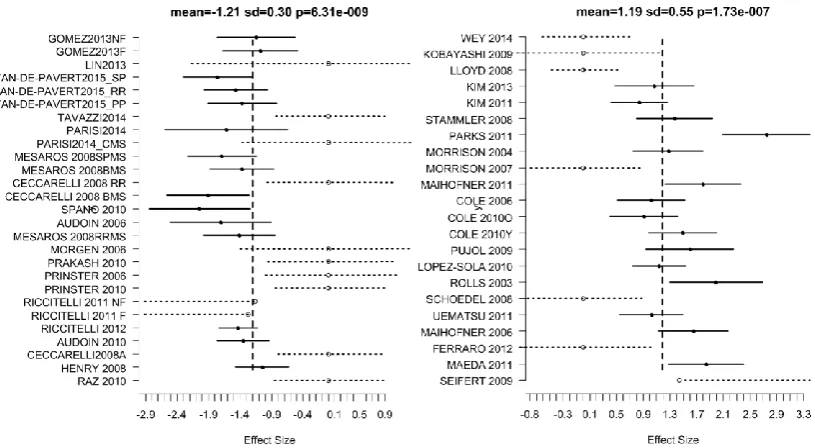
Plots of grand mean, between-study standard deviation, and regression coefficient against their

maximum likelihood estimates are shown in figure (1). MLE has been successful, over a pertinent

range of parameter values, in the presence of censoring typical of whole-brain neuroimaging studies.

Figure 1. Utility of MLE to estimate the model parameters in the presence of censoring at Z>379 (p≤0·0001). Estimates, as expected, are more accurate for many studies.

4.2 Validation of clustering distance

To consider how sensitive ClusterZ is to , numerical simulation was used. Experiments with 20

subjects were simulated with activation Z scores normally distributed with a mean of 379 and

standard deviation 10; truncated to a maximum of 60 to avoid unrealistically large values from the

tails of the normal distribution. The Z scores were truncated below 379 so that half of the generated

coordinates were censored on average. This censoring simulates a large effect [26] to avoid false

negatives as the purpose here is to demonstrate the clustering method, rather than the sensitivity of the

ClusterZ. Each study included an average, after censoring, of 10 randomly (uniformly from a GM

mask) distributed coordinates, and up to 5 (depending on the censoring) coordinates spatially

distributed about known clustering points; this spatial distribution was Gaussian, using a standard

deviation of the distances from the centre points of 45mm corresponding to a higher limit (least

dense) of standard deviations measured in clusters detected in CBMAs [26]. Three experiments were

generated with 20, 50 and 100 studies representing small to large meta-analyses. Clustering was

performed with ()=05, ()=01, and ()=005 for each number of studies. It was expected that

for smaller clustering distances the clusters would fail to form. Clustering was also performed for

fixed clustering distance, with  deduced such that ()=05 for the 20 study experiment. For this

fixed  it was expected that the clusters would grow by erroneously recruiting the random coordinates

as the number of simulated studies was increased.

Erroneous inclusion of coordinates to clusters, or erroneous exclusion of coordinates from clusters,

may make interpretation more difficult, and at least some such errors are inevitable at the edges of

clusters where the coordinates truly belonging to the clusters are closest to those that do not belong.

As well as being an issue for interpretation, these errors can bias the estimated effect sizes. To

consider the bias an experiment involving two clusters was devised, each with standard deviation of

coordinate distance from the cluster centre of 45mm as above; low density clusters with standard

deviation of 8mm are also considered. The Z scores are drawn from a normal distribution with mean

magnitude of 379 and standard deviation of 10, one cluster having negative mean and one positive;

with 20 subjects this is an effect size magnitude of 379/20=085. Between the clusters 20 random

coordinates per experiment were generated, half of which had a positive mean Z of 379, and half with

negative 379. As above all Z scores were censored below a magnitude of 379 and capped at

magnitude 60. The clusters were placed at three different distances relative to each other, ranging

from being placed at distance in different hemispheres to touching. The number of studies considered

fraction. It was expected that for small () the clusters would fail to form and the effect size would

be underestimated. At the limit of large overlap fraction it was expected that random coordinates

would be recruited to the clusters and reduce the estimated effect size because of the different effect

signs. With the clusters close together it was expected that large overlap fraction (large clustering

distance) would cause the clusters to merge resulting in an underestimated mean effect size because of

the different effect signs.

4.2.1 Validation of clustering distance Results

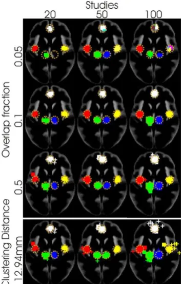
Figure (2) shows the effect of the clustering distance; note that the ClusterZ depicts clusters as +

markers for each member coordinate, rather than as a cluster of voxels, making them appear

somewhat blocky. As expected when the overlap fraction is ()=005 the clusters can fail to form

because  is too small for coordinates to overlap, and where they do form they can be fractured. For a

wide range of () (01 to 05) the clusters successfully form so, at least for this data, the method is

not overly sensitive to the clustering distance. This is because the coordinates in the true clusters are

generally considerably more densely packed than the between cluster coordinates.

The important feature of the adaptive clustering scheme is that the clusters are generally independent

of the number of studies in the analysis. This does not hold when the clustering distance is held fixed,

as seen on the bottom row of figure (2). Fixing the clustering distance causes recruitment of the

between-cluster coordinates into the true clusters as the density increases with the number of studies;

this is most evident from an increased inclusion of coordinates outside of the cluster boundary for 100

studies and clustering distance 1294mm. This leads to a paradoxically increasing number of false

positives for larger meta-analyses. It is important to note that this is not a feature specific to ClusterZ,

as it will affect any method employing a fixed FWHM; the clustering distance equivalent. Indeed this

has previously been shown to happen in the ALE algorithm [17, 26].

Figure 2. Showing the effect of clustering distance on simulated data with 5 clusters. Significant clusters are represented by + markers for each coordinate in the cluster, and different clusters are indicated by different colour markers; the boundaries of the true clusters are indicated by dashed-line

circles. For small overlap fraction (top), clusters can fail to form or be fragmented as indicated by multiple colours within-cluster. For fixed clustering distance (bottom), the clusters grow to erroneously include study specific coordinates. Importantly, allowing the clustering distance to vary

with the number of studies produces similar results for large (100 studies) and small (20 studies) meta-analyses.

In figure (3) the overlap fraction is plotted against estimated effect size to show the impact of varying

clustering distance. When the two opposite effect size clusters are well spatially separated (figure

(3a)) the plots are quite independent of the number of studies; despite the clustering distances for the

different numbers of studies being different. For very small () the clusters fail to form and the

effect sizes are underestimated; this is the same feature seen in figure (2). At the other extreme large () results in an underestimated effect size due to recruitment of between cluster coordinates; again

this is seen in figure (2). Once the coordinates are fully formed the effect size estimate is accurate, but

with increasing bias as the overlap fraction increases, and at ()=05 there is some underestimation.

This bias increases ever more rapidly as () increases, as does the standard error of the estimate. It

would appear that for smaller bias a smaller value of cluster fraction is preferable, but this comes at

the expense of an increased risk of lower density clusters not forming. This can be seen in figure (3a)

As the clusters are placed closer together, another phenomenon becomes apparent. For large

clustering distance it is not possible for the clustering algorithm to resolve two nearby clusters. In

figure (3b) this impacts the 20 study experiment mostly as the larger clustering distances cause

coordinates in the two clusters to overlap. This is even more obvious when the clusters slightly

overlap (row c), where only the experiment with 100 studies is able to properly resolve the two

clusters with an overlap fraction of 05. When clusters of opposite effect size are not resolved the

effect estimate due to the combined coordinates may be near zero, and consequently no significant

cluster would be declared. However, this can be detected by inspection of forest plots (see figure (9)),

where the mixing of positive and negative effects would be highlighted. A solution employed by other

algorithms is to perform separate positive and negative reported effect meta-analyses, but this is not

ideal as the effects are not independent. The solution offered by ClusterZ is to modify the clustering

algorithm such that only coordinates of the same effect sign can overlap, producing positive effect

clusters and negative effect clusters with no sign mixing. The application of this to the touching

clusters is shown in figure (3d), which shows the bias has been eliminated and the clusters are

resolved. There is a caveat to this modification, however, in that it can mask true heterogeneity in

reported effects. This modified algorithm should therefore only be used if the forest plots indicate

Figure 3. Showing the impact of overlap fraction (and therefore clustering distance) on effect size estimates. Two clusters are simulated, as depicted on the left; the clusters are placed at distance, near, or overlapping. True effect sizes are +085 and -085, and between cluster coordinates have the same magnitude effect. Here S.E.M is the standard error on the effect size estimate. Coordinates are placed with a standard deviation of 45mm from the cluster centre, or 8mm for the low density example.

4.3 Type 1 error control

To confirm that FCDR controls the FWER under the null hypothesis, pseudo experiments were

generated by randomly placing coordinates, independently and with uniform probability, within a GM

mask. This simulation used 40 studies, and the Z scores were sampled at random from a Gaussian

distribution with mean 379, standard deviation 10, and truncated such that 379≤|Z|≤6; this simulates

Z scores from studies reporting significant and censored activation (for example). Therefore,

incidental clusters formed by the random coordinates may be expected to have a significant positive

mean, yet there should be few significant results with FWER control. Five hundred such experiments

were analysed and the number that produced significant results counted while controlling the FCDR

expected that the pseudo experiments would produce significant results around 1%, 5%, and 10%,

respectively, of the time.

Control of the FWER is important, but does not then place a quantifiable limit on the number of

clusters, from those declared significant, that might be expected under the null hypothesis. This is an

aim of FCDR. To test this, experiments involving known numbers of true clusters (1, 3, and 5) were

simulated; with 500 simulations per experiment. Since the point of the experiment is control of false

positive results, forty studies were simulated, providing sufficient statistical power to avoid many

false negative results. As above, all Z scores were sampled at random from a Gaussian distribution

with mean 379, standard deviation 10, and truncated such that 379≤|Z|≤6. Each study had twenty

random coordinates, which was reduced to 10 on average after censoring. Added to these were a set of

true clusters distributed about fixed Talairach [27] coordinates; the spatial distribution was Gaussian,

using a standard deviation of the distances from the centre points of 45mm corresponding to a higher

limit (least dense) of standard deviations measured in clusters detected in CBMAs [26].

To compare with the ALE and ES-SDM algorithms, 50 experiments were generated (as detailed

above) for each of 0, 1, 3, and 5 fixed clusters and saved in the ALE and ES-SDM formats; these files

are included as supplemental material. The distributions of clusters detected using ALE and ES-SDM

were plotted as histograms, along with equivalent results from ClusterZ using the experiments

detailed above with FCDR 005. FDR of 005 was used with a minimum 200mm3 _{cluster size for ALE}

[26], and the recommended settings (uncorrected p-value 0005, minimum cluster size 10 voxels, and

a minimum Z threshold of 1) were used with ES-SDM [14]; in addition the default anisotropic

smoothing kernels were employed [28]. Ideally the recommended cluster based threshold method

would have been employed with the ALE algorithm, but the execution time (around one day per

experiment) prevented its use for the 200 experiments performed. Nevertheless, the limitations of

FDR in the context of CBMA are well understood [26] and can be considered in the comparison.

4.3.1 Type 1 error control Results

Five hundred pseudo experiments, with zero fixed clusters, were processed. A histogram of the

number of clusters detected are shown in figure (4). At FCDR of 001 the total number of experiments

declaring significant clusters was 9/500, which is an estimated FWER of 0018. Similarly at FCDR of

005 and 01 the total number of experiments declaring significant clusters was 24/500 and 54/500

respectively, representing family wise error rates of 0048 and 011. This experiment suggests that

FCDR is able to control the FWER under the null hypothesis, just as the FDR scheme it is based on.

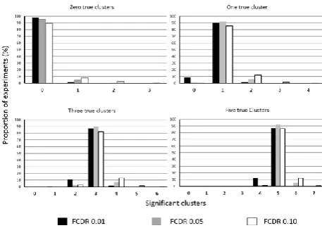
The ability of FCDR to control the type 1 error rate was also tested in experiments with up to 5 true

significant clusters, and also shown in figure (4). The number of clusters declared significant was

FDCR of 001, the number of false positives was highest for 01, while the typical setting of 005 fell

between the two. This experiment demonstrates that, at least for the simulated data, FCDR does

control both the FWE rate and the cluster-wise type 1 error rate.

Figure 4. The number of clusters declared significant by ClusterZ for known numbers of clusters (0, 1, 3, and 5) and FCDR (001, 005, and 01).

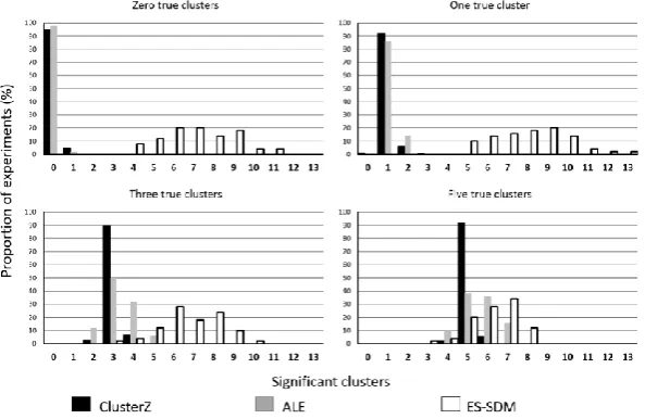
The results of the comparison between ClusterZ and the ALE and ES-SDM algorithms is shown in

figures (5) & (6). The ALE algorithm controls the FWER when there are zero true clusters since FDR

was used, but the rate of false positive clusters begins to increase for 3 and 5 clusters. However, these

extra clusters were small and are a known consequence of voxel-wise FDR in ALE. Taking into

account the limitations of voxel-wise FDR, the ALE algorithm performs similarly with ClusterZ for

this data, as can be seen in figure (6), where the small false clusters are highlighted; note the

smoothness of the ALE algorithm is due to the Gaussian kernel used by the method, while ClusterZ

depicts significant clusters by + markers for each coordinate contributing to the cluster. The ES-SDM

algorithm, on the other hand, has been unable to demonstrate control of either the FWE rate, or the

number of false clusters. This is probably a result of the uncorrected p-value threshold employed.

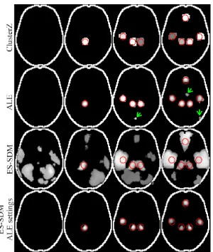
Figure (6) shows the extent of the issue, with multiple clusters detected under the null hypothesis

(zero true clusters) and results that are quite different to both ALE (despite the same coordinates being

used) and ClusterZ, and also not constrained to the regions where the true clusters are placed.

The contrast in clusters produced by ES-SDM, on the one hand, and ClusterZ and ALE on the other,

is expected to be due to the parameters being set for different aims. The ALE algorithm attempts to

model the spatial probability distribution of activation foci on a voxel-wise basis [7]. A statistical

threshold applied to this probability reveals voxel clusters that might then be loosely interpreted as the

distribution of reported activation foci. ClusterZ also attempts to find the distribution of reported

coordinates (activation and deactivation), but by clustering coordinates rather than voxels. ES-SDM

possible, to incorporate statistical parametric maps into the analysis [14]. As a consequence the

clusters are much larger than those of ALE and ClusterZ.

To consider whether the differences in clusters between ES-SDM and ClusterZ/ALE might be

completely explained by the differences in parameters, a set of equivalent (as far as is possible)

parameters values were established to reflect those used by the ALE algorithm: p-value threshold due

to FDR, the FWHM, and the minimum cluster volume. These parameters were then used with

ES-SDM, and the analysis shown in figure (6) repeated. For zero, one, three, and five clusters, the

threshold p-values were 00, 4410-6_{, 1}₇₁₀-5_{, and 2}₉₁₀-5 _{respectively in the respective ALE}

analyses; however ES-SDM allows a minimum p-value threshold of 1010-5_{, which was therefore}

used where necessary. The FWHM was set to 10mm, and the minimum cluster size 200mm3_{; these}

are similar to those typically used in ALE. There is no equivalent of the anisotropic kernels or Z value

threshold in ALE, so they were set to isotropic and the default Z>1. The results shown in figure (6)

(bottom row) demonstrate that using similar parameter settings modifies the output of ES-SDM to be

similar to ALE, and ClusterZ, for this experiment. However, this is at the expense of changing the

original aim of the method.

Figure 5. Comparison of ClusterZ, ALE, and ES-SDM using simulated data with known numbers of clusters. For ClusterZ an FCDR of 005 was employed, and FDR of 005 with a minimum cluster size

Figure 6. Typical results of numerical experiments with fixed numbers of clusters superimposed onto an axial outline of the brain. The red circles indicate the placement of coordinates belonging to the fixed clusters. The resulting significant clusters are shown as maximum intensity projections. For the ALE results, the arrows indicate small false clusters due to the use of voxel-wise FDR. The results for

ES-SDM are shown with the default parameter settings and with settings equivalent to those used by ALE (bottom).

4.4 Coordinate Based Random Effect analysis of real data

Numerical experiments verify the functionality of the algorithms and demonstrate their features, but it

remains to be shown that ClusterZ performs on real data. Full meta-analyses are a study in themselves

and beyond this demonstration, so data adapted from two previously published analyses [29, 30] are

used. The first is a meta-analysis of VBM studies of clinically isolated syndrome (CIS) and multiple

sclerosis (MS); subjects diagnosed with CIS are at risk of developing clinically definite MS, which is

known to result in grey and white matter atrophy. The studies compared grey matter density or

volume of patients to healthy controls. In total there are 21 studies reporting 29 experiments

comparing patients to healthy controls, and of these 4 were CIS, 16 RRMS, 3 BMS, 2 SPMS, 2

PPMS, 1 classical MS, and 1 cortical MS; details are in supplement 2. The second is a meta-analysis

of fMRI studies of mechanically induced pain in healthy volunteers. These studies compared

functional activation under painful stimulus to activation at rest or innocuous stimulus. In total this

performed using ClusterZ (FCDR 005 & FWE 005), ALE (default cluster forming threshold

p<0001, cluster-level FWE 005, 1000 iterations), and ES-SDM (default uncorrected p<0005,

minimum cluster size 10 voxels, Z>1, and anisotropic smoothing kernels).

ClusterZ reports its results in several ways. Cluster images use colour coding to show each significant

cluster, and the reported foci are indicated by + markers. Details of each cluster are tabulated,

including effect size estimates, cluster centroid, and Talairach labels as detailed in [31] to locate the

anatomy implicated. ClusterZ does not work voxel-wise, so the cluster volumes typically reported by

both the ES-SDM and ALE methods are not directly computable. However, an equivalent voxel-based

volume is estimated by filling an image array with overlapping cube markers for each reported

coordinate to form a solid cluster of voxels with computable volume that encompasses the distribution

of reported foci; these volumes are also reported. An important aspect of MA is data checking and

forest plots are the standard way to visualise the data in context, which is invaluable for quickly

identifying problems. Data checking is particularly important for ClusterZ, where multiple

meta-analyses (one per cluster formed) are performed. The use of random effects meta-analysis in clusters

means that forest plots become viable, and code (written for the R statistical package [32]) to draw the

plots is automatically generated for each cluster detected regardless of significance level. Forest plots

4.4.1 Real data CBRES Results

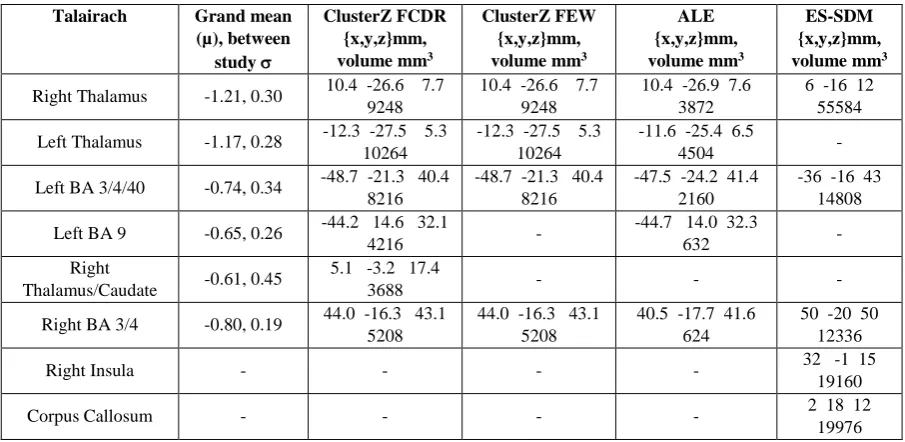
ClusterZ detected 6 significant clusters in the MS data using FCDR, which are listed in table 1. Most

covered more than one Talairach structure as indicated in the table. Using ClusterZ FWE method

reduced the significant clusters to 3, but it is worth noting that they are identical to the respective three

from the FCDR analysis; clusters, formed by the clustering algorithm, are independent of the

threshold level in ClusterZ unlike voxel-wise analyses. The ALE algorithm has declared 5 significant

clusters in in the MS data, which are very similarly located to those detected by ClusterZ. The

similarity between the ALE and ClusterZ results extends somewhat to the characteristic cluster

shapes, as can be seen by comparing rows a & b with row c in both figure (7) and figure (8), however

the ALE clusters tend to be smaller. This is a result of the different way that ALE represents clusters

(voxel-wise activation likelihood measure) compared to ClusterZ. Comparison with the ES-SDM

algorithm is not straight forward. ES-SDM declares clusters that are comparatively large, and having

different centroids; this is evident from both figure (7) and (8). The relatively large clusters reflect the

different aim of ES-SDM compared to ALE and ClusterZ. Where possible the reported cluster

centroids were matched to those detected by ClusterZ and ALE and reported in table 1.

ClusterZ declared 9 significant clusters with the pain data using FCDR; table (2) and figure (8). A

useful feature of ClusterZ is that the FCDR is estimated for every cluster, and post-hoc analysis

revealed a tenth cluster just beyond significant at FCDR 006; ClusterZ automatically estimates, and

reports, FCDR and FWE rates for every cluster detected. This is reduced to 7 clusters when FWE is

employed. ALE agreed on 8 of these. Again the ES-SDM results were somewhat different, and

matching cluster centres in table 2 was not possible for most.

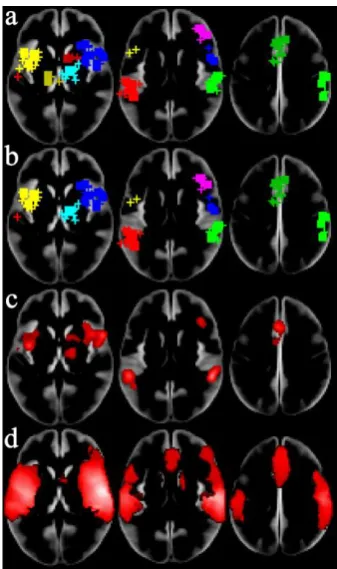
Figure (9) shows forest plots from the most significant clusters from the MS and pain analyses. These

indicate the reported effect sizes and a range deduced from the within-study standard deviation, an

overall estimate of grand mean and standard deviation, and the p-value for the cluster. Censored

studies are also depicted in the plots by empty circle markers and dashed line range indicators derived

from the study thresholds. For censored studies the markers do not indicate the contribution to the

estimate of the model parameters, but the dashed lines indicate the range over which the contribution

Talairach Grand mean (µ), between

study 

ClusterZ FCDR {x,y,z}mm, volume mm3

ClusterZ FEW {x,y,z}mm, volume mm3

ALE {x,y,z}mm, volume mm3

ES-SDM {x,y,z}mm, volume mm3

Right Thalamus -1.21, 0.30 10.4 -26.6 7.7 9248

10.4 -26.6 7.7 9248

10.4 -26.9 7.6 3872

6 -16 12 55584

Left Thalamus -1.17, 0.28 -12.3 -27.5 5.3 10264

-12.3 -27.5 5.3 10264

-11.6 -25.4 6.5

4504 -

Left BA 3/4/40 -0.74, 0.34 -48.7 -21.3 40.4 8216

-48.7 -21.3 40.4 8216

-47.5 -24.2 41.4 2160

-36 -16 43 14808

Left BA 9 -0.65, 0.26 -44.2 14.6 32.1

4216 -

-44.7 14.0 32.3

632 -

Right

Thalamus/Caudate -0.61, 0.45

5.1 -3.2 17.4

3688 - - -

Right BA 3/4 -0.80, 0.19 44.0 -16.3 43.1 5208

44.0 -16.3 43.1 5208

40.5 -17.7 41.6 624

50 -20 50 12336

Right Insula - - - - 32 -1 15

19160

Corpus Callosum - - - - 2 18 12

19976 Table 1. Significant clusters with their estimated grand mean effect size and between-study standard deviation, volume, and centre Talairach location, for the MS data. The results are shown to compare

ClusterZ, ALE, and ES-SDM methods.

Talairach Grand mean (µ), between

study 

ClusterZ FCDR {x,y,z}mm, volume mm3

ClusterZ FEW {x,y,z}mm, volume mm3

ALE {x,y,z}mm, volume mm3

ES-SDM {x,y,z}mm, volume mm3

Left BA 13/40 1.20, 0.56 -52.3 -28.9 19.9 13512

-52.3 -28.9 19.9 13512

-52.2 -27.5 20 5760

-

Right BA 13/44 1.18, 0.21 41.3 8.4 10.1 21920

41.3 8.4 10.1 21920

41.3 9.7 6.8 6472

-

Right BA 40 1.17, 0.27 53.2 -25.1 26.0 12048

53.2 -25.1 26.0 12048

52.3 -24.4 20.5 3832

-

Left BA 13 1.1, 0.27 -38.2 5.3 11.3 14520

-38.2 5.3 11.3 14520

-38.2 1.9 10.4 4432

-

Right BA 9/10/46 0.75, 0.54 36.7 37.3 23.7 6264

36.7 37.3 23.7 6264

36.3 39.2 24 1144

-

Right Thalamus 0.82, 0.58 13.4 -12.6 9.6 8208

13.4 -12.6 9.6 8208

12.9 -12.7 9.7 1672

-

Right Caudate/putamen

0.67, 0.62 13.4 6.5 5.4 4832

- 14.6 6.9 5.2

1160

-

Right BA 6/8/24 0.91, 0.37 -2.0 17.6 40.1 15248

-2.0 17.6 40.1 15248

-1.6 17.8 38.8 5072

-3 22 42 28120 Left Thalamus 0.65, 0.15 -10.9 -17.7 5.7

4136

- - -

Right BA 7/40 *0.56, 0.56 *38.5 -55.7 47.4 3336

- - -

Right BA 44/45/48 - - - - 51 -5 13

110088

Left BA 40/41/48 - - - - -38 -13 8

76352

Undefined - - - - 11 -1 22

2296 Left Caudate

Nucleus

- - - - -11 6 18

792 Table 2. Significant clusters with their estimated grand mean effect size and between-study standard deviation, volume, and centre Talairach location, for the pain data. The results are shown to compare

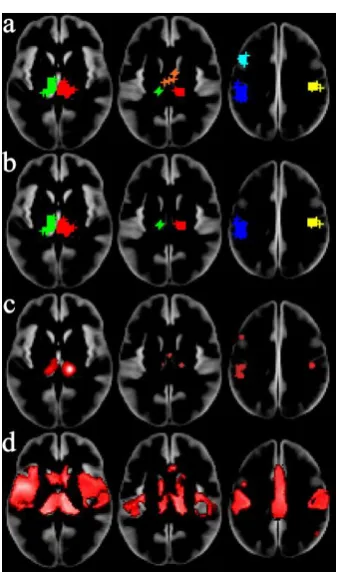
Figure 7. Significant clusters detected in the MS coordinates. a) is ClusterZ using FCDR 005, b) is ClusterZ using FWE 005, c) is ALE algorithm employing p<0001 cluster forming threshold and

cluster threshold of 005 (FWE corrected), and d) is ES-SDM using the recommended p<0005 threshold and cluster extent of 10 voxels. For the ClusterZ results coordinates contributing to clusters

Figure 8. Significant clusters detected in the pain coordinates. a) is ClusterZ using FCDR 005, b) is

ClusterZ using FWE 005, c) is ALE algorithm employing p<0001 cluster forming threshold and

cluster threshold of 005 (FWE corrected), and d) is ES-SDM using the recommended p<0005

threshold and cluster extent of 10 voxels. For the ClusterZ results coordinates contributing to clusters

Figure 9. Forest plots of the effect sizes in the most significant cluster from the MS (left) and pain

(right) meta-analyses. Solid circle markers indicate the effect size reported by the study in the cluster,

while the confidence intervals are depicted as solid horizontal lines spanning ±1.96 times the within

study standard deviation of the effect size. Censored values are indicated by open circle markers and

the intervals by dashed lines (---o---); these are determined by the study thresholds and indicate

5

Discussion

Here a method of performing coordinate based random effect meta-analysis and meta-regression was

presented. ClusterZ utilises the Z scores (or t statistics) and coordinates, typically reported by

functional MRI or VBM studies, to detect where studies report effects consistently. The reported

statistics are not suitable effect measures for meta-analysis directly, but they can be transformed

(equations 1-5) into an approximate effect size that is suitable for a random effects meta-analysis. The

advantages of ClusterZ include estimates of effect size, the possibility of meta-regression, and that

cluster-wise statistical significance is determined by the reported effect rather than the density of

clustering, which is not so interpretable. Furthermore, analysis at the cluster-, rather than voxel-, level

makes type 1 error control using the easy to interpret false cluster discovery rate feasible.

ClusterZ relies on multiple established methods to perform its analysis. Firstly, clusters are formed

based on the DBSCAN algorithm, which aims to differentiate true clusters from study specific effects.

The clustering algorithm has a parameter that is analogous to the FWHM parameter in CBMA

algorithms, but in ClusterZ this automatically adapts to the experiment to avoid false negatives when

there are few studies and avoid false positives when there are many studies; the fixed FWHM used in

other algorithms paradoxically increases the false positives for increasing numbers of studies.

Estimation of model parameters is based on the standard statistical technique of maximum likelihood

estimation, which also allows for censoring. The subsequent inference on the parameters is based on

the generalised likelihood ratio test, which has well known statistical properties in the asymptotic

limit. Finally, principled control of the false positives clusters is based on the popular FDR method,

which controls the FWER under the null hypothesis, and then limits the proportion of clusters

expected under the null hypothesis to a user specified level; by comparison the ES-SDM method

employs no disciplined control of the false positive clusters. This is perhaps the most important

feature of ClusterZ, since false positives results might propagate and even amplify the very issues that

motivated the meta-analysis in the first place.

Maximum likelihood estimation is used to estimate model parameters in the presence of censoring.

MLE is one of multiple methods of performing meta-analysis, and has been shown to perform well in

comparison [33]. Numerically MLE is a nonlinear problem, with no guarantee of convergence to the

correct solution. However, because ClusterZ computes estimates only at clusters, rather than voxels,

the algorithm is very efficient (~1minute for typical analyses such as the MS and pain studies) so

considerable computations effort is dedicated to finding the global maximum solutions. Numerical

experiments confirmed its validity, being able to accurately estimate the parameters of the models