The CAPTAIN Toolbox for System Identification, Time Series Analysis, Forecasting and Control: Guide to TVPMOD: Time Variable Parameter Models

The C

APTAIN

T

OOLBOX

for System

Identification, Time Series Analysis,

Forecasting and Control

Guide to TVPMOD

Time Variable Parameter Models

Handbook Part 2

3 July 2017

AUTHORSHIP

Current developers:

Dr. Wlodek Tych and Emeritus Prof. Peter C. Young

Lancaster Environment Centre (LEC), Lancaster University, Lancaster, LA1 4YQ, United Kingdom.

Dr. C. James Taylor

Engineering Department, Lancaster University, Lancaster, LA1 4YR, United Kingdom.

Co-author:

Prof. Diego J. Pedregal

Escuela Tenica Superior de Ingenieros, Industriales Edificio Politenica, Campus Universitario s/n, 13071 Ciudad Real, Spain.

Additional contributors:

GLOSSARY

ACF Autocorrelation Function AR Auto-Regression

ARMA Auto-Regression Moving-Average

ARIMA Auto-Regression Integrated Moving-Average ARX Auto-Regression with eXogenous variables BSM Basic Structural Model

DAR Dynamic Auto-Regression

DARX Dynamic Auto-Regression with eXogenous variables DBM Data-Based Mechanistic

DHR Dynamic Harmonic Regression DLR Dynamic Linear Regression DTF Dynamic Transfer Function FIS Fixed Interval Smoothing GRW Generalised Random Walk IRW Integrated Random Walk KF Kalman Filter

LLT Local Linear Trend ML Maximum Likelihood

NAN Not-A-Number

NMSS Non-Minimal State Space NVR Noise Variance Ratio

PACF Partial Autocorrelation Function PIP Proportional-Integral-Plus RIV Refined Instrumental Variable

RIVSID Refined Instrumental Variable System Identification (CAPTAIN folder)

RW Random Walk

SDARX State Dependent Auto-Regression with eXogenous variables SDP State Dependent Parameter

SDTF State Dependent Transfer Function SISO Single Input, Single Output

SRIV Simplified Refined Instrumental Variable SRM Smoothed Random Walk

SS State Space

TDC True Digital Control

TDCONT True Digital CONTrol (CAPTAIN folder) TF Transfer Function

TVP Time Variable Parameter

CONTENTS

Chapter 1 Introduction 1

Chapter 2 State Space models 4

Chapter 3 Unobserved Components models 30

Chapter 4 Time Variable Parameter models 57 Chapter 5 State Dependent Parameter models 81

The CAPTAIN Toolbox is a collection of MATLAB functions for non-stationary time series analysis, forecasting and control. The toolbox is useful for system identification, signal extraction, interpolation, forecasting, data-based mechanistic modelling and control of a wide range of linear and non-linear stochastic systems. The toolbox consists of three modules, organised into three folders (or directories) as follows:

 TVPMOD: Time Variable Parameter (TVP) MODels. For the identification of unobserved components models, with a particular focus on state-dependent and time-variable parameter models (includes the popular dynamic harmonic regression model).  RIVSID: Refined Instrumental Variable (RIV) System Identification algorithms.

For optimal RIV estimation of multiple-input, continuous- and discrete-time Transfer Function models.

 TDCONT: True Digital CONTrol (TDC). For multivariable, non-minimal state space control, including pole assignment and optimal design, and with backward shift and delta-operator options.

The present document is a guide to the TVPMOD module. The chapter headings in this guide follow a logical structured progress through the relevant methodology, using worked examples. TVP modelling is introduced in Chapter 2. Here, the filtering algorithm, smoothing algorithm, generalised random walk model and hyper-parameter optimisation routines are described. Chapter 2 presents the models in their most general state space form, while the following three chapters introduce various special cases, namely: unobserved component models in Chapter 3; dynamic regression models in Chapter 4; and state dependent parameter models in Chapter 5.

1.1 Use of the CAPTAIN Toolbox

1. Wherever the CAPTAIN Toolbox has been used to generate results which have then been used in any written work, please reference it using the text below:

Taylor, C.J., Pedregal, D.J., Young, P.C. and Tych, W. (2007) Environmental Time Series Analysis and Forecasting with the Captain Toolbox, Environmental Modelling and Software, 22, pp. 797-814 (http://dx.doi.org/doi:10.1016/j.envsoft.2006.03.002). 2. The CAPTAIN Toolbox is supplied in good faith and whilst all efforts have been made

to assure that it is free from errors and bugs, the authors and Lancaster University accept no liability for erroneous results obtained through the use of the Toolbox.

3. Installation of the CAPTAIN Toolbox is carried out at the user’s own risk and neither the authors nor Lancaster University accept any responsibility in the unlikely event of installation resulting in detrimental effects to the user's computer hardware or software. 4. The user may not redistribute the Toolbox to any third party.

5. Ownership of the Toolbox is retained by the authors. The web download is an evaluation copy of the Toolbox. If you wish to continue using the Toolbox beyond the evaluation period, please contact C. James Taylor at the address below.

E-mail: [email protected]

Web: http://www.lancs.ac.uk/staff/taylorcj/

6. Any part of the CAPTAIN Toolbox may be used for scientific or educational purposes. For commercial applications, permission is required from the authors.

7. CAPTAIN is provided without formal support, although questions and bug reports can be emailed to the authors.

1.2 Getting Started

For installation instructions and toolbox overview, please see the Getting Started Guide. Since CAPTAIN is largely a Command Line toolbox, it is also assumed that the reader is already familiar with basic MATLAB usage, such as loading data and plotting graphs. To obtain a full list of user functions, type help tvpmod in the Command Window, replacing ‘tvpmod’ if necessary with the actual name of the folder (directory) chosen when you first installed the toolbox. To illustrate, the first few lines of the function list are:

>> help tvpmod Captain Toolbox

Time Variable Parameter Models

Unobserved Components Models.

dhr - Dynamic Harmonic Regression analysis. dhropt - DHR hyper-parameter estimation.

irwsm - Integrated Random Walk smoothing and decimation. irwsmopt - IRWSM hyper-parameter estimation.

Figure 1.1 Demos for the TVPMOD module obtained by typing tvpdemo at the MATLAB Command Line.

To open the Command Line demos for the TVPMOD module,

>> tvpdemo

A straightforward graphical user interface provides access to the demos (see Fig. 1.1). The latter utilise the Command Window for input and output, as well as generating graphs in a separate Figure Window, so make sure both of these are visible. Demo scripts can be opened in the MATLAB editor.

Each function includes help information obtained in the usual manner e.g. help irwsm. Note that default input arguments are shown in parenthesis while (*) implies no default (hence a user input argument is always required for this variable). Some functions include more information, readable using e.g. type irwsm or edit irwsm (see Chapter 3). Finally, entering the function name without any arguments summarises the calling syntax.

1.3 Caveat

This chapter introduces one of the main methodological tools in CAPTAIN, namely the State

Space (SS) model. Indeed, most of the models in the toolbox, though not all, are implemented in such a SS form. Originating from the state-variable method of describing differential equations, the SS approach has subsequently been developed for modelling by researchers in many different scientific disciplines and is, perhaps, the most natural and convenient approach for use with computers. It is a general and flexible tool that encompasses numerous time series models.

In fact, a number of models uniquely available in CAPTAIN are inherently based on such

state space methods and, therefore, always require a SS formulation. This includes the entire category of Time Variable Parameter (TVP) models considered in Chapter 4. There are other practical situations in which it is particularly convenient, though not essential, to also use a SS model, e.g. when there are missing values in the time series or when interpolation, forecasting and backcasting operations are required. Finally, in certain cases, the SS form simply offers a solution that is identical to other, sometimes better known, conventional approaches.

For these reasons, whenever a SS form is necessary or convenient, CAPTAIN uses it, while

in a few exceptional cases, it is avoided because other superior approaches are available. For example, the instrumental variable method for the estimation of fixed parameter Transfer Function (TF) models (in the SYSID module of CAPTAIN) replaces the state

space- based Maximum Likelihood (ML) approach by default, unless the latter is specifically chosen. However, such issues are usually transparent to the user, since

CAPTAIN chooses the optimal modelling strategy internally.

The present chapter provides an introduction to SS methods and may, therefore, be regarded as the broad theoretical basis for the special cases discussed subsequently. In this regard, a number of standard topics are briefly covered, typical of many publications and

CHAPTER 2

textbooks in this field. However, several aspects are novel and exclusive to CAPTAIN and

these are highlighted in the text where appropriate.

Almost all of the modelling functions in CAPTAIN might be quoted in this chapter because

they are particular cases of the general SS framework! However, to help the reader digest the general principles, we will restrict the present discussion to the simplest possible models, leaving the more advanced cases for subsequent chapters. In this regard, the key modelling functions covered below are irwsm and irwsmopt, while fcast, reconst, acf and histon are also introduced for data preparation and diagnostics. Together, these tools are useful for exploratory analysis or in situations where the a priori knowledge about the system is minimal, as will be seen in the later worked examples.

2.1 The State Space framework

A SS system is composed of two sets of equations, namely: (i) the so called State Equations (represented as a single equation in vector-matrix form below), that reflect all the dynamic behaviour of the system by relating the current value of the states to their past values, together with any deterministic and stochastic inputs; and (ii) the Observation Equation that defines how these state variables are related to the observed data. Although there are a number of different SS formulations possible, the one favoured in CAPTAIN is:

t t t

1 -t t

+e y

t x

H

G Fx

x 



 _

t

1

: Equation n

Observatio

: Equations

State 

(2.1)

where y_t is the stochastic observed variable; x_t is an n dimensional stochastic state vector; t

η is an k dimensional vector of system disturbances; and e_t is a vector of zero mean white noise variables (measurement noise). F ,GandH_t are, respectively, the nxn, nxk, and

1xn non-stochastic system matrices.

The following assumptions apply to this system:

 η_t~iid N



0,Q



; e_t~iid _N



_0,2



_;



_η



_0

t t,e

cov .

 The initial stochastic state x₀ is independent of η_t and e_t for every t.

 The system matrices F ,G ,H_t ,Qand2 are known (or have been previously estimated in some way) whereas the initial conditions for the states and their covariance matrix (x₀ and P₀ respectively) are unknown.

Error (see e.g. Young, 1984; or Harvey, 1989). In CAPTAIN, these recursive algorithms are

the Kalman Filter (KF; Kalman, 1960) and Fixed Interval Smoothing (Bryson and Ho, 1969), as discussed in Section 2.2 below.

Numerous results may be found in the literature for various relaxations of the above conditions (see e.g. Durbin and Koopman, 2001). One particularly straightforward and useful case is when the gaussianity assumptions on the perturbations are dropped. In this case, the state estimates provided by the KF/FIS are still optimal in the sense that they minimise the mean square error within the class of all linear estimators.

The Generalised Random Walk model

The following Generalised Random Walk (GRW) model, which is one of the simplest SS models based on (2.1), is used extensively in CAPTAIN,

                            t t t t t t x x x x 2 1 1 2 1 1 2 1 0     





_       t t t _x x T 2 1 0 1 (2.2)

Here,  , and are constant parameters; T_t is a smoothed signal component consisting of the first state x_1t; and x_2t is a second state variable (generally known as the ‘slope’); while _1t and _2tare zero mean, serially uncorrelated white noise variables with constant block diagonal covariance matrix Q, as stated in the general formulation above.

This model subsumes a number of special cases that have received specific names in the literature. The main ones are the Random Walk (RW:  1;   0; _2t 0); Smoothed Random Walk (0  1;   1; _1t 0); the Integrated Random Walk (IRW:     1; _1t 0); the Local Linear Trend (LLT:     1); and the Damped Trend (  1; 0  1).

When any one of these options is combined with additive noise in an observation equation, the resulting time series model might be called a ‘GRW plus noise’ model. One such case is the ‘RW plus noise’ model, ideal for the estimation of a time varying mean. Here, the SS representation takes the following form:

t +e x y x x t t t t    _{ } t 1 1 : Equation n Observatio : Equation State  (2.3)



t



t t e L y     1 1  (2.4)

Similarly, the ‘IRW plus noise’ model, useful for extracting smooth trends to non-stationary time series, may be developed as follows,





+et

x x y x x x x t t t t t t t                                     2 1 t 1 1 2 1 1 2 1 0 1 : Equation n Observatio 1 0 1 0 1 1 : Equations State  (2.5)

Here, the two state equations that may instead be written as,









2 1

1 2 1 1 1       t t t t x B x x B  (2.6)

In this case, substituting the second state equation into the first, and then into the observation equation, we obtain the reduced form,



t



t

t e L y     2 2 1  (2.7)

This IRW model with observational noise will be utilised in Example 2.1 below. First, however, an algorithm for the estimation of the states is required.

2.2 State Estimation

1. Forward Pass Filtering Equations Prediction: T G GQ F P F P x F x r T t t t t t t        1 1 | 1 1 | ˆ ˆ ˆ ˆ

Correction: (2.8)













| 1

1 1 | 1 | 1 | 1 | 1 1 | 1 | 1 | ˆ ˆ 1 ˆ ˆ ˆ ˆ ˆ 1 ˆ ˆ ˆ                  t t t T t t t t T t t t t t t t t t t T t t t t T t t t t t t y P H H P H H P P P x H H P H H P x x

2. Backward Pass Smoothing Equations







 





t N t t



t t t t t T t t N t t t t T t t T T t T t t t t T r N t N t y P F P P P P F P P P x H H L F H H P I L L G GQ x F x ˆ ˆ ˆ ˆ ˆ ˆ ˆ ˆ } ˆ { ˆ ˆ ˆ 1 | 1 | 1 | 1 1 | 1 | 1 1 1 1 1 1 1 1 | 1 1 |                          (2.9)

with L_N 0. Note that the FIS algorithm is in the form of a backward recursion operating from the end of the sample set to the beginning. The main difference between the KF and FIS algorithms (2.8)-(2.9) utilised in CAPTAIN, and more conventional filtering/smoothing

algorithms found in some other toolboxes, are the nxn Noise Variance Ratio (NVR) matrix Q_r and the nxn matrix ˆ P _t defined below,

2

 Q

Q_r  ; ₂

* ˆ ˆ t t P

P  (2.10)

Here, _ˆ*

t

P is the error covariance matrix associated with the state estimates xˆ . In most of _t the models implemented in CAPTAIN, the NVR matrix Q_r is diagonal.

Forward Pass Filtering

For a data set of T samples, the KF algorithm (2.8) runs forward and returns a ‘filtered’ estimate of the state vector and its covariance matrix (xˆ and _t Pˆ , respectively) at every t sample t, based on the time series data up to sample t. These estimates are computed in two steps. In the first instance, the one step ahead forecast for the mean value of the state vector and its covariance matrix (xˆtt₁ and Pˆtt1, respectively) are obtained from the prediction

equations, using the model alone. Secondly, these estimates are updated by means of the correction equations, as each new data sample becomes available.

contrast, the current estimate of the covariance matrix itself, does not depend on either the state estimates or the data, but only on the model and the previous estimate of the covariance matrix. Another noteworthy point, is that significant saving in computational effort are obtained in CAPTAIN by the realisation that repeated operations are involved in

the calculation of the required estimates, especially in the correction equations.

There are two intermediate variables calculated by the KF that are of particular importance (as will become clear in the following section 2.3), namely:

T t t t t t

t t t t t f

y v

H P H

x H

1 |

1 |

ˆ 1 ˆ

ˆ ˆ

  

 

 _(2.11)

The first term above is the innovations sequence, or the one-step-ahead forecasting errors of the model, while the second is the variance of these innovations, where the latter are equal to the variance of the one-step-ahead forecasts. Both variables are scalar, so that the matrix inversions required in the KF correction equations are actually very simple in computational terms. The normalised innovations are used in many diagnostic tests, since, recalling the original formulation of the SS model (2.1), they should be iid_N



_0,2



_{in a}

correctly specified model.

When missing data are encountered within the data set, the correction equations are redundant and missing samples are effectively interpolated by using the filtered estimates. In the same manner, forecasts may be produced by artificially adding ‘missing’ data at the end of the series. In this case, the values of vˆ and _t fˆt outside the sample span are now the true multiple-steps-ahead forecasting errors and associated variance respectively, and may be used for computation of the confidence intervals.

Fixed interval smoothing

The FIS algorithm in (2.9) normally runs backwards after the filtering step and yields a ‘smoothed’ estimate of the state vector and its covariance matrix based, at every sample t, on all T samples of the data. This means that, as more information is used in the FIS algorithm with respect to the KF estimates, its Mean Square Error cannot be greater. When missing data are encountered, an interpolation is generated based on the data at both sides of the gap. Finally, if the missing observations are at the beginning of the sample, the FIS algorithm generates backcasts of the time series.

The FIS algorithm (2.9) is utilised by many software packages and is the default so called ‘Q-algorithm’ in CAPTAIN. However, an additional FIS algorithm is also available

argument can be changed to select this alternative ‘P-algorithm’, obtained by replacing the first equation in (2.9) by,

1 |

1 | ˆ ˆ

ˆtN xt t PtFTLt

x (2.12)

Here, the new estimates of the state vector are based on the filtered ones, while in (2.9) it is calculated recursively from the previous estimate of the state vector. Furthermore, (2.12) does not require inversion of the F matrix. Both algorithms are discussed in detail by previous publications (see e.g. Young, 1984; Harvey, 1989; Ng and Young, 1990).

Example 2.1 Estimation of a trend for the air passenger series

The simple IRW plus noise model (2.7) has long been used for smoothing time series in the economics literature. It is equivalent to the well-known Hodrick-Prescott filter (HP; Hodrick and Prescott, 1997). This filter has been used by many researchers in the area of empirical business cycles, and the similarities between both filters was highlighted long ago (recently reviewed by Young and Pedregal, 1996).

Many researchers use fixed values of the smoothing constant depending on the frequency rate of the data. In CAPTAIN, however, the relationship between the smoothing constant

(the NVR in this context) and the cut-off frequency properties of the low-pass filter is made explicit, and is easily generalisable to any type of model in SS form. The advantage is that the user may choose the NVR according to their particular needs and the properties of the data, it is not fixed by any prior conceptions. For example, given the RW family of models defined by (cf. (2.6) and (2.7)),





j t j t

t e

L

y 



 

1



(2.13)

the cut-off frequency for 50% of spectral power is given by,

   

  

 j

w arccos 1 0.5NVR1 (2.14)

with ₂

2

NVR

 _

 (Young and Pedregal, 1996).

In this case, Q_r in equation (2.10) is the scalar state noise variance 2



NVR Period (time samples) Years (quarterly series) Years (monthly series)

10 2.86 0.71 0.24

1 6.01 1.51 0.51

0.1 11.02 2.76 0.92

0.01 19.78 4.95 1.65

0.001 35.28 8.82 2.94

1/1600 39.69 9.92 3.31

[image:15.595.106.516.71.169.2]

0.0001 62.81 15.71 5.23

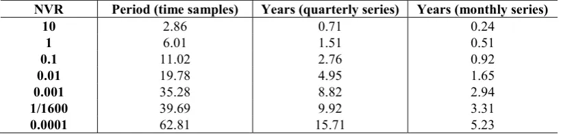
Table 2.1 Relationship between the NVR parameter and the associated bandwidth of the IRW filter, i.e. the minimum period of cycles included in the filtered series.

Table 2.1 suggests that for a NVR value of 0.001, the smoothed signal would contain all the information of the original signal from a period of 35.28 samples up to infinity. All periods below that value are filtered out.

Put another way, if a signal has to be estimated such that it contains all the information of the original series for approximately 5 years and above, a NVR of 0.01 would be the option for a quarterly series, while 0.0001 should be chosen for a monthly series.

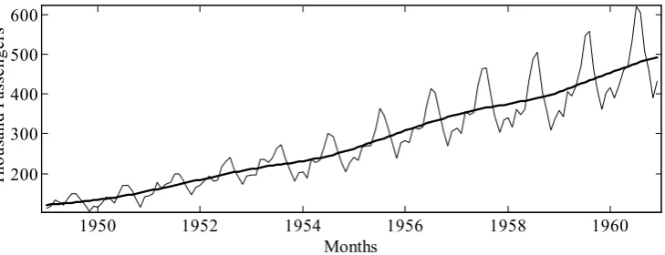
To illustrate these points, consider again the well-known air passenger series introduced in Chapter 1 (Box and Jenkins, 1970, 1976). Figure 2.1 illustrates these data, together with two possible trends obtained from different NVR values (0.1 and 0.0001). This graph may be obtained in CAPTAIN by entering the following MATLAB® code,

>> load air.dat

>> t1 = irwsm(air, 1, 0.1); >> t2 = irwsm(air, 1, 0.0001); >> t = (1949 : 1/12 : 1961-1/12)'; >> plot(t, [air t1 t2]);

1950 1952 1954 1956 1958 1960

200 300 400 500 600

T

ho

us

an

d

Pa

ss

en

ge

rs

[image:15.595.103.485.445.673.2]

Months

Which one of these trends is the best? Although this is clearly a subjective matter, we may still say something about Figure 2.1, based on a general idea of what we mean by a trend. In particular, with the higher NVR of 0.1, the smoothed signal follows the data too closely to be regarded as a ‘trend’ in the normal sense, since it includes cyclic behaviour with a period of less than one year, i.e. it is really a combination of a trend and a seasonal component, something that in principle is undesirable. By contrast, with NVR = 0.0001, the smoothed signal does not appear to combine the trend and seasonal component in this manner, and so is more ‘correct’ in a signal decomposition sense.

In statistical terms, a more suitable approach would be to model the whole series with an Unobserved Components (UC) model, rather than attempt to extract the trend alone. Of course, this is also the main approach utilised in CAPTAIN and is described in Chapter 3.

Nonetheless, CAPTAIN does offer the opportunity to just estimate a trend in this simple,

exploratory context, using objective criteria for NVR optimisation, as discussed below.

2.3 (Hyper-) Parameter Estimation

The recursive KF and FIS algorithms above both require knowledge of all the system matrices F ,G ,H_tandQ_r. In this regard, depending on the particular structure of the model chosen, there will be a number of elements either known prior to the analysis or fixed by the user. For example, if a RW model is specified, then clearly  1 and   0 in the SS model (2.2). However, in most cases, some unknown elements or hyper-parameters

will remain unspecified and must be estimated separately. Typically, these include the NVR matrix Q_r. In the following discussion, we will summarise all these hyper-parameters, whatever variables they may represent, in the vector .

The hyper-parameter estimation problem is completely different to the state estimation problem and, in a certain sense, entirely independent of it. This fact is clearly seen in the range of methods available in the literature, some of which do not use the SS form at all! The most common methods include: Maximum Likelihood (ML) in the time domain (Schweppe 1965; Harvey, 1989); ML in the frequency domain based on a Fourier transform (Harvey, 1989; pages 191-204); alternative approaches in the frequency domain (Ng and Young, 1990; Young et al., 1999); combinations of all the previous methods (Young and Pedregal, 1999); Bayesian approaches (West and Harrison, 1989); and estimation methods based on the reduced ARIMA form (Hillmer and Tiao, 1982; Hillmer

et al., 1983; Maravall and Gómez, 1998).

A selection of the most useful methods are implemented in CAPTAIN and listed below.

cases, several methods are available for the same type of model, with the one considered optimal as the default option (refer to the on-line help for each particular function).

 Time domain ML estimation for UC, TVP and State Dependent Parameter (SDP) models (Chapters 3, 4 and 5). This is the most widespread estimation method in the SS context, mainly because of its strong theoretical basis and because it is the most well known approach in many other areas of statistics. For this reason, it is discussed in detail below. See also Examples 2.2 and 2.4 below.

 Minimisation of the multiple-steps-ahead forecasting errors, also discussed below. This heuristic method is very useful when other methods do not provide a satisfactory answer to the problem, or when the objective of the research is strongly based on the forecasting performance of model. See also Examples 2.2 and 2.3 below.

 Frequency domain estimation, based on the spectral properties of the model (Young

et al., 1999). The parameters are estimated so that the logarithm of the model spectrum fits the logarithm of the empirical pseudo-spectrum (either an AR-spectrum or periodogram) in a least squares sense. A full description of this algorithm can be found in Chapter 3.

 Sequential Spectral Decomposition, reserved for a certain class of unobserved components models, i.e. Trend plus Auto-Regression (AR) also discussed in Chapter 3. This approach consists of decomposing the original series into quasi-orthogonal components, taking advantage of the exceptional spectral properties of the smoothing algorithms mentioned above. The overall non-linear problem is decomposed into several linear or quasi-linear steps, each solved in fully recursive terms. This yields a simple solution, with some loss of optimality from the ML viewpoint, but has proven to be very successful in practise. As a final step, filtering and smoothing are repeated using the whole SS formulation based on the analysis completed in the previous steps.

 Instrumental variable estimation of transfer function models in discrete and continuous time, as primarily implemented in the RIVSID module of CAPTAIN.

Because some of the methods mentioned above have been developed for specific models, their description is conveniently postponed to future chapters. In the present chapter, however, two general methods that are not intrinsically linked to particular models are reviewed, namely ML and the minimisation of the multiple-steps-ahead forecasting errors. Maximum Likelihood

Assuming that all the disturbances in the SS form are normally distributed, the required Log-likelihood function can be computed using Kalman Filtering via ‘prediction error decomposition’ (Schweppe 1965; Harvey, 1989). The appropriate function for the general SS model in equation (2.1) is, therefore,

 

_

_

 

 

 

 T

t t t T

t

t

f v f

T L

1 2

1 ˆ

ˆ 2 1 ˆ log 2 1 2 log 2

log  (2.15)

where T is the number of observations, while vˆ and _t fˆt are the innovations and their variance respectively (see equation (2.11)), computed directly from the KF algorithm. A number of issues must be taken into account when maximising (2.15); see e.g. Harvey, (1989) and Koopman et al. (2000). In the first place, the gradient and hessian necessary to find the optimum by numerical procedures can be evaluated either analytically or numerically, while the standard errors of the estimates may be found by means of the hessian, as is usual in the literature. Secondly, in the present context, it is usual to maximise the so called concentrated likelihood. This is because it is always possible to concentrate out one of the variances in _2 _{or Q, reducing by one the number of}

parameters to estimate. In CAPTAIN, 2 is always the concentrated out variance, as shown

initial condition problem, is to incorporate the distribution of the initial conditions into the likelihood function itself, which yields the exact likelihood function, independent of such conditions and useful for short length time series (see e.g. De Jong, 1988, 1991; Casals et al., 2000). In CAPTAIN, the simplest diffuse priors option is chosen by default, although the

user may always intervene and specify xˆ₀ and Pˆ₀ directly.

Finally, a consideration common to all the estimation procedures in CAPTAIN,is that it is

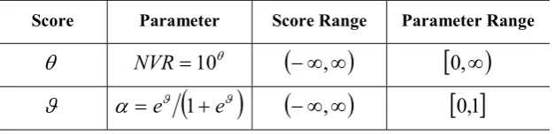
common to estimate the scores (certain transformations of the hyper-parameters) rather than the hyper-parameters themselves. Such parameters are then constrained to a certain domain in order to avoid nonsensical results. Two typical examples are that the NVR values should always be positive, while the  parameters in SRW models should always lie between zero and one inclusive. In this regard, the NVR and  scores used in CAPTAIN

are listed in Table 2.2.

Score Parameter Score Range Parameter Range

 _NVR10



_,





_0,



[image:19.595.164.478.311.387.2]

 _{ e}



_1e





_,



 

_0,1

Table 2.2 Hyper-parameters and scores in CAPTAIN.

In this way, the searching algorithm for ML looks for an unconstrained value of the scores from minus infinity to infinity, and it is transformed into a valid value of the corresponding hyper-parameters. The disadvantage when the scores are estimated rather than the parameter themselves is that the distribution of the scores is normal, according to theory, while the distribution of the parameters is, in general, not known. However, confidence intervals may always be reconstructed by applying the same transformation to the confidence interval of the scores.

Limitations of ML

There is no doubt that ML has theoretical and practical advantages. Its optimal properties are well-known and it is a widely applicable method for SS models. Indeed, the objective function (2.15) is applicable to any model written in SS form. The only requirement is that the user has to determine the appropriate form of the system matrices necessary to specify the model in SS terms. However, since CAPTAIN uses SS models as standard, this is not a

problem in the present context.

Despite the advantages of ML on theoretical grounds, it does have some disadvantages, hence other methods are also implemented in CAPTAIN for specific types of model. In

dimension of the model, since the recursive algorithms must be used to compute the Log-likelihood function at each iteration in the numerical optimisation. Furthermore, problems are sometimes encountered when the theoretical hypothesis on which the model is based does not hold in practice. An instructive example is the case of transfer function models when the input signal is a deterministic variable (such as steps, impulses, ramps, etc.). For this particular problem, however, the RIVSID module of CAPTAIN offers instrumental

variable methods instead, which outperform ML and are never worse in other standard situations (Young, 1984).

Also, it is well-known (e.g. Young et al., 1999) that in certain UC models, the likelihood surface can be quite flat around its optimum, making the practical optimisation problem very inefficient at best and impossible in some cases. This is one important reason why these models usually have to be constrained when estimated by ML (we will come back to this issue in Chapter 3: see the examples therein). By contrast, for example, estimation methods in the frequency domain are free from these difficulties. In this regard, the approach implemented in CAPTAIN for UC models, optimises the hyper-parameters so that

the minimisation of the multiple-steps-ahead forecasting errors discussed in the next subsection.

Given the pros and cons of each method, it is possible to improve overall model estimation by combining methods for different components of the model, i.e. to use the most appropriate method for each component. This is the approach suggested for SDP models for which, when necessary, frequency objective functions and ML are used together. SDP modelling is a very general procedure for the identification of non-linear relationships of many kinds. In this approach, an iterative procedure known as back-fitting is used. Here, parts of the model are estimated conditional on fixed values of the rest of parameters. In each iteration, the most appropriate estimation method can be used, either in the frequency domain or ML in the time domain.

Minimisation of the multiple-steps-ahead forecasting errors

The log-likelihood function (2.15) is dependent on the one-step-ahead forecasting errors, i.e. vˆt  yt Htxˆt_|t₁, a natural outcome of the KF solution. However, the multiple -step-ahead forecasting errors can also be computed by simply repeating the KF prediction equations, say h times, without applying the correction equations. The associated forecasting errors are then as follows,

 

t t tt h t h y

vˆ  H xˆ _| (2.16)

This equation computes the forecasting errors at each t with all the information available up to t-h. Given these errors, one interesting option for hyper-parameter estimation is to minimise the sum of the squares of the h-step ahead errors, i.e.



 







 

 

  

 T

h n t

h t t t t h

n t

t h y

v

1

2 | T

1 2

ˆ =

ˆ

= Hx

J (2.17)

This approach is a natural heuristic extension to ML and may be applied when the latter does not provide a sensible solution to certain problems.

2.4 Worked examples

The following examples illustrate the basic functionality of hyper-parameter estimation in

CAPTAIN, and show how the toolbox may be utilised for the preliminary analysis,

Example 2.2 Hyper-parameter estimation for the air passenger series

Following directly from Example 2.1 above, consider again IRW smoothing of the air passenger series.

For some initial conditions, ML estimation does not yield useful results for this data set (Pedregal et al. 2007). This is because the theoretical properties assumed about the IRW model are not fulfilled by these particular data. In effect, the model (2.5) assumes that the perturbations about the trend are uncorrelated white noise, while it is clear here that the innovations are not at all white noise, indeed they are strongly periodic (see Figure 2.1). As a consequence, if the model is defined as an IRW model alone, then ML estimation can sometimes yield an unacceptable solution e.g. returning a very high NVR and a ‘smoothed’ signal that is almost identical to the original series.

However, irwsmopt uses an initial frequency domain estimation step, in order to obtain improved initial conditions for the subsequent ML estimation. For the present example, this approach yields satisfactory results, as indicated by the output shown below.

>> load air.dat

>> nvr = irwsmopt(air, 1, 'ml');

FREQUENCY DOMAIN INITIAL CONDITION ESTIMATION METHOD: FREQUENCY DOMAIN. AR-SPECTRUM(24) OPTIMISER: LSQNONLIN

0.016 seconds.

PER. RW NVR Score S.E. Alpha Score S.E. 0.00 1.0 5.1196e-03 -2.2908 0.100 1.0000 - - Frequency Domain Objective Function: 2875.485

METHOD: MAXIMUM LIKELIHOOD OPTIMISER: FMINSEARCH

Date: 24-Jun-2017 / Time: 21:19 0.219 seconds.

PER. RW NVR Score S.E. Alpha Score S.E. 0.00 1.0 4.990e-06 -5.3019 - 1.0000 - - Likelihood: -750.466

Since irwsmopt is designed for straightforward smoothing applications, there are no user settings associated with the frequency domain initialisation step, and MATLAB® may

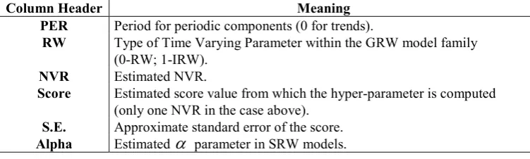
For information, Table 2.3 summarises the displayed tabular output from irwsmopt, while the header and footer above also confirm the optimisation method, the core MATLAB®

function being utilised, the time taken to complete the optimisation and the Likelihood. Other hyper-parameter optimisation routines in CAPTAIN, including dhropt, dlropt,

daropt, darxopt, dtfopt and univopt follow a similar convention. Note that the MATLAB®

optimisation function (fminsearch in the example above) is automatically selected by

CAPTAIN, depending on the optimisation method chosen and the presence other MATLAB®

toolboxes installed on the users system, although this default can be overwritten (refer to the toolbox function help information).

Column Header Meaning

PER Period for periodic components (0 for trends).

RW Type of Time Varying Parameter within the GRW model family

(0-RW; 1-IRW).

NVR Estimated NVR.

Score Estimated score value from which the hyper-parameter is computed (only one NVR in the case above).

S.E. Approximate standard error of the score.

[image:23.595.114.490.249.362.2]

Alpha Estimated  parameter in SRW models.

Table 2.3 Tabular outputs from CAPTAIN hyper-parameter estimation functions.

Returning to the present example, an alternative to ML is to minimise the 12 steps ahead forecasting errors, as shown below. In general, the number of samples in a year, or the number of samples in any sort of cycle in the data, should be utilised in such optimisation.

>> nvr = irwsmopt(air, 1, 'f12');

METHOD: SUM OF SQUARES OF 12-STEPS-AHEAD FORECAST ERRORS OPTIMISER: FMINSEARCH

0.672 seconds.

PER. RW NVR Score S.E. Alpha Score S.E. 0.00 1.0 5.5777e-04 -3.2535 - 1.0000 - - Sum of Squares of 12-Steps-Ahead Forecast Errors: 268133.0759

>> tr = irwsm(air, 1, nvr);

>> t = (1949 : 1/12 : 1961-1/12)'; >> plot(t, [air tr])

For brevity, the frequency domain initialisation results are omitted from the output shown above (and in later examples). The NVR obtained in this case is 0.000558, with an associated cut-off period of 3.4 years (Table 2.1), returning the trend illustrated by Figure 2.2. Finally, it is straightforward to generate forecasts of the trend by adding nan values (MATLAB® Not-A-Number variables) to the end of the data, either by using standard

1950 1952 1954 1956 1958 1960 200

300 400 500 600

T

ho

us

an

d

Pa

ss

en

ge

rs

[image:24.595.119.484.79.219.2]

Months

Figure 2.2 Air passenger data and trend chosen by minimising the 12-steps-ahead forecasting errors.

1950 1952 1954 1956 1958 1960

200 300 400 500 600

T

ho

us

an

d

Pa

ss

en

ge

rs

Months

Figure 2.3 Air passenger data, trend and trend forecasts for the last year of data.

>> nvr = irwsmopt(air(1 : 132), 1, 'f12'); >> tr = irwsm(fcast(air, [133 144]), 1, nvr); >> plot(t, [air tr]);

>> hold on

>> plot([t(132) t(132)], [0 650])

For illustrative purposes, the analysis above does not use the final year of the air passenger series, just the first 132 samples. Instead, the trend is forecasted for this year and compared with the original series, as illustrated in Figure 2.3, where the vertical line shows the forecasting horizon. It should be stressed that data to the right of the forecasting horizon are not used in the analysis, neither for estimating the NVR nor for smoothing the time series. Nonetheless, even with this simple IRW model, the forecasted trend is sensible, showing the long term behaviour of the series continuing in the correct direction.

Example 2.3 Interpolation and variance intervention for steel consumption in the UK

In order to illustrate the variance intervention and missing data handling capabilities of

CAPTAIN, the quarterly steel consumption in the UK, measured in thousands of metric tons,

[image:24.595.115.485.265.404.2]

the estimate of Pˆ_t|t1 in the prediction equation (2.8) is ‘reset’ to a large value, implying a lack of confidence in the estimates at that sample.

In order to plot the steel consumption with a correct time axis, as in Figure 2.4 below, enter the following MATLAB® commands:

>> load steel.dat

>> t = (1953.75 : 0.25 : 1992.75)'; >> plot(t, steel)

1955 1960 1965 1970 1975 1980 1985 1990

200 300 400 500

T

ho

us

an

d

M

et

ri

c

T

on

s

[image:25.595.106.486.210.375.2]

Quarters

Figure 2.4 UK steel consumption from 1953Q4 to 1992Q4.

The anomalous large consumption figures in the first and second quarters of 1980 (referred to subsequently as 1980Q1 and 1980Q2) were due to strikes in the sector. Furthermore, two apparent falls in the mean level of steel consumption can be observed in 1975Q2 and 1980Q1. One way of handling these problems at the simple exploratory level is to smooth the series, assuming missing data (again, MATLAB® Not-A-Number values) for the strikes

and setting variance intervention points at 1975Q2 and 1980Q1, as shown below.

>> y = fcast(steel, [106 107]);

>> nvr = irwsmopt(y, 1, 'f12', [87 106], [], 2);

METHOD: SUM OF SQUARES OF 12-STEPS-AHEAD FORECAST ERRORS OPTIMISER: LSQNONLIN

0.516 seconds. 2 missing values

PER. RW NVR Score S.E. Alpha Score S.E. 0.00 1.0 6.390e-05 -4.1945 - 1.0000 - - Sum of Squares of 12-Steps-Ahead Forecast Errors: 1756523.4294

Although not necessary for this example, the sixth input argument to irwsmopt illustrates how to change the MATLAB® optimisation function. In particular, the example above

utilises lsqnonlin, which assumes that the MATLAB® Optimisation Toolbox is installed.

The graphical output of this analysis is illustrated in Figure 2.5, where the jumps in the trend at the variance intervention points can be clearly seen and the perturbation about the trend (lower plot) appropriately shows that there are no remaining jumps in the series.

1955 1960 1965 1970 1975 1980 1985 1990

250 300 350 400 450 500

T

ho

us

an

d

M

et

ri

c

T

on

s

Months

1955 1960 1965 1970 1975 1980 1985 1990

-50 0 50

T

ho

us

an

d

M

et

ri

c

T

on

s

[image:26.595.115.486.212.514.2]

Months

Figure 2.5 UK steel consumption, trend and perturbation about the trend.

Finally, it is sometimes interesting to reconstruct the data by assuming that the jumps in the trend did not occur, as shown below. Here, the CAPTAIN function reconst serves as a tool

to remove the jumps, with the new estimate of the trend added to the perturbation signal. The value of such a calculation will be shown later in Chapter 3.

1955 1960 1965 1970 1975 1980 1985 1990 300

350 400 450 500 550

T

ho

us

an

d

M

et

ri

c

T

on

s

[image:27.595.116.485.91.215.2]

Months

Figure 2.6 UK steel consumption with the jumps in the trend removed.

Before moving to the final example, it is useful to first introduce the Autocorrelation (ACF) and Partial Autocorrelation (PACF) Functions, together with the Ljung-Box test, since these will be utilised below and occasionally in later chapters.

Autocorrelation (ACF) and Partial Autocorrelation (PACF) functions

The ACF and PACF are two key identification tools, very useful for detecting time structure dependence in any time series. Popularised by Box and Jenkins (1970), they have been extensively used by time series analysers ever since. The aim is to determine the linear correlation coefficients between a time series and the lagged values of the same series. The representation of these coefficients against the lag, usually in the form of a bar diagram, is the ACF or Correlogram. More formally, the theoretical ACF of a stationary process y_t (i.e. constant mean and variance) is defined as,

0

2 _

 



 k

y k

k   k 0,1,2, (2.18)

where,









t y t k y



k E y  y 

   _  k0,1,2, (2.19)

Here, _k is the autocovariance function that measures the covariance between a time series and its past, while _y and 2

y

 are the (constant) mean and variance of the process, respectively. The ACF is symmetrical around lag k 0, so only positive values for the lag are considered.

Several estimators have been proposed in the literature, including the sample equivalents of the population counterparts, i.e.,

0 2 _c

c s c

r k

y k

with,







0,1,2,

1

1   



  _

 y y y y k k

T

c T k _{t k}

t t

k (2.21)

where T is the number of samples and y is the sample mean. Note that, if the time series is white noise, an approximation of the variance of the autocorrelation estimators is,

 

T r

Var _k  1 k 0,1,2, (2.22)

Equation (2.22) may be used to test the significance of any individual coefficient, i.e. any coefficients bigger than twice the standard error will be considered significantly different from zero.

The previous estimators are equivalent to the following set of linear regressions fitted to the data,                    kt k t k k t t t t t t t e y r y e y r y e y r y     2 2 2 2 1 1 1 1 (2.23)

where _i and e_it (i1,2,,k) are a set of constants and gaussian white noise terms, respectively. These equations are simply AR models of increasing orders, with all the intermediate parameters constrained to zero.

Apart from the individual test for each ACF parameter quoted above, a summary test of autocorrelation up to order m is the Ljung-Box test (Ljung and Box, 1978), given by the statistic,





     m k k k T r T T Q 1 2

2 (2.24)

This is distributed as a _2 _{with m1 degrees of freedom under the null hypothesis of no}

autocorrelation.

                        kt k t kk t k k t t t t t t t t e y y y e y y y e y y           1 1 2 2 22 1 21 2 1 1 11 1 (2.25)

The PACF is a representation of the coefficients _ii (i1,2,,k) against the lag. The variance of these coefficients are given by equation (2.22), or they may be computed as the standard error of the estimators in the previous set of regressions.

The ACF, PACF, their standard errors and the Q test are all computed by the CAPTAIN

function acf. For example, Figure 2.7 is the output of the following code, where the ACF and PACF are estimated for a sequence of gaussian random numbers.

>> acf(randn(200, 1), 10);

m acf desv Q Prob m pacf desv 1 -0.0199 0.0707 0.0808 - 1 -0.0199 0.0707 2 -0.0306 0.0707 0.2713 0.6025 2 -0.0310 0.0707 3 -0.0798 0.0708 1.5781 0.4543 3 -0.0812 0.0707 4 -0.0251 0.0713 1.7076 0.6353 4 -0.0298 0.0707 5 -0.0688 0.0713 2.6888 0.6112 5 -0.0759 0.0707 6 0.0505 0.0716 3.2207 0.6660 6 0.0390 0.0707 7 0.0481 0.0718 3.7060 0.7164 7 0.0415 0.0707 8 0.0721 0.0720 4.7987 0.6845 8 0.0663 0.0707 9 -0.0143 0.0723 4.8420 0.7743 9 -0.0041 0.0707 10 0.0245 0.0723 4.9700 0.8369 10 0.0343 0.0707

The 2nd input argument to acf is the number of autocorrelation coefficients required by the user. As would be expected for white noise, Figure 2.7 shows that the series has no autocorrelation: the bars are all well within the standard errors (dotted trace). The same conclusion is strongly supported by the Q statistic and its probability value for any value of m, shown by the 4th and 5th columns above.

0 4 8

-0.1 0 0.1 ACF C or re la ti on

0 4 8

-0.1 0 0.1 PACF C or re la ti on

Example 2.4 Time variable mean estimation for volume in the Nile river

Sometimes a debate arises among researchers about whether the mean level of a certain variable is changing over time or not. Numerous tests and procedures have been developed in order to investigate such a hypothesis. In this regard, if the stochastic behaviour of the signal about the time varying mean is approximately uncorrelated white noise, then there are some particularly simple and well formalised options. This is the case for the RW plus noise model introduced above. Here, the smoothed signal or trend is effectively a time varying mean variable that is assumed to evolve as a RW, while the rest of the signal is assumed white noise. Clearly, more complex options may be pursued by adding specific models to describe the perturbation about the trend if necessary, as discussed in Chapter 3. Consider, for example, the Nile river annual volume measurements from 1871 to 1970 measured in 108 _{cubic meters, illustrated in Figure 2.8.}

>> load nile.dat

>> t = (1871 : 1970)'; >> plot(t, nile)

1870 1880 1890 1900 1910 1920 1930 1940 1950 1960 1970

600 800 1000 1200

Years

10

e8

m

3

Figure 2.8 Annual volume of the Nile River in 10e8 cubic meters.

These data were analysed by Cobb (1978) and Balke (1993), among others. The key issue here is to determine whether there is a systematic decline in the level from 1899 onwards (sample 29), a feature that seems visually apparent from the figure. To investigate, the RW plus noise model is estimated as shown below, with the output illustrated in Figure 2.9. For brevity, detailed optimisation results from irwsmopt are omitted from the text below and the later examples (incidentally, the other hyper-parameter optimisation routines in the toolbox have an option to turn off tabular and graphical output if desired).

>> nvr = irwsmopt(nile, 0, 'ml') nvr =

0.0924

1870 1880 1890 1900 1910 1920 1930 1940 1950 1960 1970 600

800 1000 1200

Years

10

e8

m

3

Figure 2.9 Annual volume of the Nile River, time variable mean and approximate 90% confidence intervals.

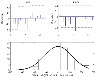
Note that the second input argument to both irwsmopt and irwsm is zero, in order to specify a RW trend, and that the NVR parameter is estimated by ML. In fact, this analysis takes advantage of the fact that, as it was seen in Example 2.2, ML will only provide a sensible solution if the theoretical assumptions about the model are fulfilled by the data. In this case, we can later check that the perturbations about the trend are indeed white noise. It is clear from Figure 2.9 that the mean level has gone down since the beginning of the century. To test the adequacy of the model in a statistical sense, we examine the perturbations by means of the sample and partial autocorrelation functions (acf), together with a plot of the histogram superimposed over a Normal distribution (histon). The latter

CAPTAIN function also returns a normality test, in the form of the Bera-Jarque statistic and

associated probability value (Jarque and Bera, 1980).

>> acf(nile-tr, 20); >> histon(nile-tr);

These graphs are illustrated in Figure 2.10. The Ljung-Box Q-test of autocorrelation for 20 lags is 17.7 indicating that there are no overall autocorrelation problems (Ljung and Box, 1978). Furthermore, the Bera-Jarque test indicates that the normality hypothesis cannot be rejected by a very wide margin. To sum up, both tests show that the theoretical assumptions about the model are fulfilled with no problem.

A second approach to the problem, which draws clearer light about the sharp decline in the level, is to use variance intervention again, directly specifying this 29th sample in the analysis, as shown below.

>> nvr = irwsmopt(nile, 0, 'ml', 29) nvr =

2.9035e-20

Figure 2.10 Analysis of the perturbations: Autocorrelation (ACF), Partial autocorrelation (PACF) and histogram of the residuals.

The estimated NVR is approximately zero, implying that the mean is constant apart from the break at the selected sample, as illustrated in Figure 2.11. Finally, although not shown here, acf and histon again indicate that the perturbations about the trend are white noise (the Q test for 20 lags is 14.35).

1870 1880 1890 1900 1910 1920 1930 1940 1950 1960 1970

600 800 1000 1200

Years

10

e8

m

[image:32.595.109.483.78.379.2]

3

2.5 Conclusions

The present chapter has introduced the state space framework that is the basis for most of the models implemented in CAPTAIN and has formally described the associated filtering

and smoothing algorithms at the heart of the toolbox. The chapter has also discussed a number of approaches for the estimation of any unknown elements or hyper-parameters in these models, concentrating on Maximum Likelihood and the minimisation of the multiple-steps-ahead forecasting errors.

Unobserved Components (UC) modelling is a general strategy for time series analysis and signal extraction, based on the assumption that the series is composed of an additive or multiplicative combination of different components that have defined statistical characteristics but which cannot be observed directly. In CAPTAIN, such components may

include a trend, cyclical components, stochastic perturbations and so on. In the statistical literature, typical approaches to UC modelling include:

 Ad-hoc methods of seasonal adjustment in which smoothing procedures are used to extract trend and seasonal components from the time series. In this regard, one of the oldest and best known techniques for signal extraction is the Census X-11 method and its later extensions X-11 ARIMA and X-12 ARIMA. See e.g. Findley et al. (1996) and the references therein.

 The ARIMA or Reduced Form approach to UC model identification and estimation, based on the assumption that the series can be modelled as an Auto-Regressive-Integrated-Moving-Average (ARIMA) model. See e.g. Box et al. (1978); Maravall and Gómez (1998). Starting from this reduced form (ARIMA) model, the UC model (considered as a structural form following the Econometrics parallel) is obtained by the imposition of a number of (arbitrary) restrictions to ensure the existence and uniqueness of the decomposition.

 The Optimal Regularisation approach, based on direct optimal estimation of the components within a regularisation context. See e.g. Akaike (1980); Young and Pedregal (1996); Hodrick and Prescott (1997). In this case, constraints are imposed on the state estimates via a Lagrange Multiplier term within the cost function, in order to ensure that they possess the required characteristics.

 The State Space (SS) approach provides a rather more obvious formulation of UC concepts and, since this is the method implemented in CAPTAIN, is discussed

in detail below. See also e.g. Ng and Young (1990); Young (1994); Young et al. (1999). Alternative SS approaches that have some points in common with

CAPTAIN, as well as a few radically different aspects, are discussed by Harrison

CHAPTER 3

UNOBSERVED

It is clear from these examples that UC modelling may be regarded as a broad philosophy, an alternative to other more traditional ways of time series modelling, rather than as a particular model form and estimation method. However, the present authors believe that the SS approach is one of the most powerful and flexible frameworks for developing UC models. Indeed, the state estimation algorithms and associated methods for hyper-parameter optimisation, introduced in Chapter 2, provide a complete solution for the identification of UC models. All that remains is to characterise each component of the model in an appropriate SS form.

The previous chapter has already discussed one of the simplest cases, namely a trend component represented by an Integrated Random Walk (IRW) plus white noise model. Here, the CAPTAIN function irwsmopt is utilised to optimise the hyper-parameters, while

irwsm provides the filtering, smoothing, forecasting and interpolation operations (see e.g. Example 2.4). Following a similar syntax, the dhr/dhropt and univ/univopt combinations

in CAPTAIN provide for a more diverse range of UC models, as discussed below. Finally,

the toolbox includes a number of functions to assist in the identification of these models, in both the time and frequency domains, namely: aic, acf, arspec and period.

3.1 General Form of the Unobserved Components Model

UC models in CAPTAIN can be synthesized by the following discrete-time equation,

 

_{N e e ~N}

 

_0,2

f S C T

y_t  _t  _t _t u_t  _t  _{t t (3.1)}

where y_t is the observed time series; T_t is a trend or low frequency component; C_t is a sustained cyclical or quasi-cyclical component (e.g. an economic cycle) with period different from that of any seasonality in the data; S_t is a seasonal component (e.g. annual seasonality); f

 

u_{t captures the influence of a vector of exogenous variables} u_t, if necessary including stochastic, nonlinear static or dynamic relationships; N_t is a stochastic perturbation model, i.e. coloured noise modelled as an Auto-Regression (AR) process; and, as shown, e_t is an ‘irregular’ component, usually defined for analytical convenience as a normally distributed Gaussian sequence with zero mean value and variance 2 (i.e discrete-time white noise).

One assumption that is maintained in every UC methodology is that all the components are orthogonal to the rest. In this context, it is noteworthy that the SS model representing equation (3.1) can be built by block-concatenation of all the matrices of each SS subsystem related to each of the components.

Despite the generality of equation (3.1), it should be stressed that in the majority of applications not all these components will be simultaneously necessary. Indeed, important identifiability problems may arise among the components if they are not defined appropriately. For example, a N_t AR component including seasonal roots will conflict severely with the seasonal component S_t if both are included in a single model. In a similar manner, unit roots in the N_t component would have problems with the trend component

T_t. For these reasons, CAPTAIN normally restricts the user to formulations of the problem

that are practically useful, so that such identification problems do not arise when using the toolbox (see examples below).

3.2 State Space form for UC Models

The SS model for each component in equation (3.1) is introduced below. Trend models (T_t)

The trend models available in CAPTAIN are all particular cases of the General Random

Walk (GRW) family of models represented by equation (2.2). These include, most commonly, the Random Walk (RW) and Integrated Random Walk (IRW) introduced in Chapter 2. A third option, the Local Linear Trend (LLT) model may be obtained by using RW and IRW models simultaneously, as shown below. The SS form of such a LLT model with observational noise is defined as follows,

                              1 2 1 1 1 2 1 1 2 1 1 0 1 1 t t t t t t x x x x  





_t t t

t _x e

x

T _

      2 1 0 1 (3.2)

The state equations may be written using the backward-shift operator as,







1



1₂ 2₂ 1₁ 1 1

1         t t t t t x L x x L   (3.3)

Then, substituting the second equation in the first one we have,





1

_

2 2

_

1 1

1

1  _{ }

 

 t _t

t

L x

L   (3.4)



t

 

t



t t e L L y        1 1 1 1 2 2 2   (3.5)

i.e. the addition of a RW and IRW model if the state noises are independent of each other (an assumption that is usual in this context).

Two further trend models, available only in the CAPTAIN functions univ and univopt for

AR + Trend analysis, are the so-called Integrated AR (IAR) or Double Integrated AR (DIAR) models. The motivation for these options arises from the observation that, for the simplest trend models, it is quite common to find correlation in the residuals. For example, when utilising an IRW model for the trend, it is assumed that its second difference will be white noise, which is not always the case in practice. IAR and DIAR models take advantage of the correlation, by building an addition model for these residuals, in order to improve the overall forecasting performance.

One caveat, however, is that it is possible for the FIS algorithm itself to induce this kind of correlation. Indeed, it can be shown (Young and Pedregal, 1996) that the correlation structure depends on the autocorrelation of the original time series itself. Nonetheless, if the second difference does show a predictable behaviour, especially if there is some physical meaning (e.g. related to the business cycle), then it would be worthwhile to try to forecast it. In this case, the DIAR model, which is defined below in a manner similar to the earlier examples, provides one particular approach,

p p t t t t t t t t L L L x x D D D T T                  2 2 1 3 1 1 1 1 1 1 (3.6)

In SS form, this model may be described by the following equations,

t t p p p t p x x x x D T x x x x D T                                                                                                  0 0 0 0 0 0 1 0 0 0 0 0 0 0 0 1 0 0 0 0 0 0 0 1 0 0 0 0 0 0 0 0 1 1 0 0 0 0 0 0 1 1 3 1 3 2 1 1 3 2 1 3 2 1                        (3.7)





t

t

The model is then fully defined by the variance of 3t and the coefficients of the AR polynomial. Although this is a rather more complex model than the GRW, it does have the capability of providing non-linear like forecasts of the trend, very useful in situations near turning points.

Cyclical and seasonal models (C_t and S_t)

Although these two types of components are given different names in equation (3.1), both can be treated in the same way from a modelling standpoint since both reflect a periodic kind of behaviour. The difference between them lies only on the period considered, with ‘seasonal’ usually reserved for an annual cycle. CAPTAIN provides two approaches for

modelling any such periodic behaviour, as discussed below.

Dynamic Harmonic Regression (DHR; Ng and Young, 1990; Young et al., 1999)

The DHR model is similar to a Fourier analysis, but with coefficients that evolve smoothly in time. The model is,

 

 







          2 0 sin cos s j t j jt j jt t t

t S e a t b t e

y   (3.8)

with,

_j j

s j       2 1 2

, s 2

, ,  (3.9)

and,                             jt jt jt jt j j j t j jt a a a a ' ' 0 ' ₁ 1 1     

NVR

 

_jt NVR

 

'_jt (3.10)

Here,

 

s 2 s 2 for even s and

 

s 2  



s 1 2



for odd s. Parameters a_jt and b_jt are represented as GRW models with the associated NVR values both equal for the same harmonic period. Note that setting ₀ 0 reduces the correspondent term for j0 to a matrix of ones and zeros, implying that GRW trends are naturally accommodated within a DHR context.